HAL Id: tel-02196913
https://tel.archives-ouvertes.fr/tel-02196913
Submitted on 9 Dec 2020
HAL is a multi-disciplinary open access archive for the deposit and dissemination of sci-entific research documents, whether they are pub-lished or not. The documents may come from teaching and research institutions in France or abroad, or from public or private research centers.
L’archive ouverte pluridisciplinaire HAL, est destinée au dépôt et à la diffusion de documents scientifiques de niveau recherche, publiés ou non, émanant des établissements d’enseignement et de recherche français ou étrangers, des laboratoires publics ou privés.
Flavor physics: precision as an avenue to discovery
Diego Guadagnoli
To cite this version:
Diego Guadagnoli. Flavor physics: precision as an avenue to discovery. High Energy Physics -Phenomenology [hep-ph]. Université de Savoie, 2014. �tel-02196913�
Auteur: Diego Guadagnoli
Affiliation:
Laboratoire d’Annecy-le-Vieux de Physique Théorique (LAPTh, UMR 5108) et
Université de Savoie Mont-Blanc
Titre: Flavor physics: Precision as an avenue to discovery
Composition du Jury:
M. Augusto CECCUCCI
M. Paolo GAMBINO (rapporteur)
M. Guido MARTINELLI
Mme. Marie-Noëlle MINARD (president, rapporteur)
M. Achille STOCCHI
Flavor physics: precision as an avenue to discovery
Diego Guadagnoli
LAPTh, Université de Savoie et CNRS, BP110, F-74941 Annecy-le-Vieux Cedex, France E-mail: diego.guadagnoli@lapth.cnrs.fr
The present manuscript describes work pursued in the years 2008-2013 on improving the Standard-Model prediction of selected flavor-physics observables. The latter include: (1) ‘K, that quantifies indirect CP violation in the K0≠ ¯K0system and (2) the very rare
decay Bs æ µµ, recently measured at the LHC. Concerning point (1), the manuscript
describes our reappraisal of the long-distance contributions to ‘K (refs. [1–3]), that have
permitted to unveil a potential tension between CP violation in the K0- and in the Bd-system. Concerning point (2), the manuscript gives a detailed account of various
systematic effects, pointed out in ref. [4] and affecting the Standard-Model Bs æ µµ
decay rate at the level of 10% – hence large enough to be potentially misinterpreted as non-standard physics, if not properly included. The manuscript further describes the multifaceted importance of the Bd,s æ µµ decays as new-physics probes, for instance
how they compare with Z-peak observables at LEP, following the effective-theory ap-proach of ref. [5]. Both cases (1) and (2) offer clear examples in which the pursuit of precision in Standard-Model predictions offered potential avenues to discovery. Finally, the manuscript describes the impact of the above results on the literature, and what is the further progress to be expected on these and related observables.
Contents
1 Introduction 2
1.1 Historical remarks . . . 3
1.2 The Standard Model: gauge sector . . . 5
1.3 The Standard Model: Higgs/Yukawa sector . . . 6
1.4 Flavor physics . . . 9
1.5 Flavor-physics bounds on beyond-SM physics . . . 11
1.6 Why pursuing flavor physics . . . 14
1.7 Content of the manuscript . . . 15
2 Indirect CP violation in the K0≠ ¯K0 system 16 2.1 Introduction to the problem . . . 16
2.2 CPV in K physics: theory vs. experiment . . . . 17
2.3 Derivation of the ‘K formula . . . 19
2.4 The Ÿ‘ correction . . . 22
2.5 A closer look at the operator-product expansion for ‘K . . . 25
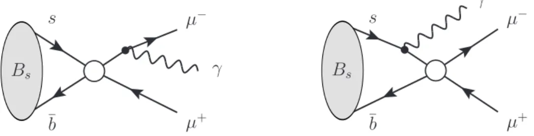
3 The rare decay Bs æ µ+µ≠ 38
3.1 Bs æ µµ within the SM: decay structure . . . . 38
3.2 Experimental status, and steps towards a precise prediction . . . 40
3.3 Renormalization-scheme dependence . . . 41
3.4 Soft-photon corrections . . . 46
3.5 Bs≠ ¯Bs oscillation effects . . . 49
3.6 Prediction for the non-radiative decay and error budget . . . 51
3.7 The Bdæ µ+µ≠ decay . . . 54
3.8 Bs æ µµ as a probe of the Yukawa sector . . . . 55
3.9 Bs æ µµ as an EW precision test . . . . 57
4 Outlook 65 4.1 Paths towards improving the accuracy of the ‘K prediction . . . 65
4.2 Bs æ µµ: outlook and possible new directions . . . . 74
1 Introduction
The Standard Model denotes the theoretical framework that, to the best of our knowledge, describes all observed phenomena whose nature is other than gravitational. We make this distinction between gravitational and non-gravitational interactions from the outset in order to remark two major, distinctive differences between the corresponding theories.
The first difference is epistemological, is namely related to the quality and extent of knowl-edge achievable ‘in principle’ in either of the two cases. The interactions described by the Standard Model have an inherently quantum character. They occur at distances, or equiva-lently energy-exchange scales, such that the phenomenon to be described is modified by the observer describing it. This circumstance introduces an intrinsic uncertainty in the knowl-edge of certain observables, summarized by Heisenberg’s Uncertainty Principle and in the resulting discrete, or quantum, nature of these observables.1 On the other hand, as far as
gravity is concerned, no evidence exists for an energy regime where a quantum description becomes necessary, so the theory of gravity is formulated in terms of classical fields, at vari-ance with the Standard Model, where a ‘quantum’ field theory is necessary. This difference is such that, in spite of huge theoretical efforts, only speculations exist on how to derive Standard Model and gravitational interactions from a common principle.
The second difference is historical. The making of General Relativity has proceeded as in the dreams of every theoretical physicist: two basic, intuitively understandable princi-ples have been worked out to their ultimate implications using only logical necessity. The beauty, consistency and solidity of the resulting construction made its proposer have little doubt about experimental confirmations, that in fact unfailingly followed. Conversely, the construction of the Standard Model has been by and large a trial-and-error process. It is maybe useful to shortly summarize this process here – this excursus2 should make at least
clear why the final product retained the modest name of Standard Model, which sounds more like a placeholder, rather than the definitive name of a fundamental theory.
1 From the argument of ‘intrinsic uncertainty’ one would be tempted to trace back quantum phenomena to
a probabilistic theory. Such attempts would however be frustrated by quantum phenomena like interference and entanglement. As a result, we have to date no fully deterministic understanding of quantum physics, as summarized by R.P. Feynman’s words: “Nobody understands quantum mechanics”.
2 I closely follow the point of view of one of the absolute protagonists of this process, S. Weinberg. See
1.1 Historical remarks
The history of the Standard Model (SM) traces back to the 1950s, where, after the triumphs of Quantum Electrodynamics, people were stuck with a non-renormalizable four-fermion theory to explain weak-interaction phenomena like — decay, and with incalculable theories for strong interactions, because the strong coupling made perturbation theory unusable. What was worse is that in either case the approach was purely phenomenological, i.e. not supported by a clear rationale. To identify a viable framework for weak interactions people tried to pursue principles of symmetry, typically with frustrating results, because most of the considered symmetries – like CP, the octet structure of hadrons, etc. – were at best only approximate, not to mention those that were badly broken, like parity. A sheer symmetry-based approach was per se not sufficient to make progress.
In this situation, among the several theoretical ideas circulating, two turned out to give a major boost towards understanding weak interactions. The first is the introduction of the idea of gauge symmetry, and its application to the construction of a renormalizable theory based on a non-Abelian group, SU(2), by Yang and Mills [7]. It should be noted, however, that people did not immediately consider applying this idea to weak interactions, for two ‘good’ reasons. First, throughout the 50s weak interactions were thought to consist not only of vector and axial-vector contributions, but also of scalar and even tensor ones, because of a number of wrong experiments. Only by the late 50s the situation was cleared up in favor of only vector and axial-vector contributions [8], that Yang-Mills (YM) gauge bosons are suitable to mediate. A second, more serious obstacle, was however the problem of how to give mass to YM gauge bosons – massless vector bosons would surely have been seen by experiment. Trying to force mass terms by hand would destroy the gauge symmetry, and make the YM theory non-renormalizable, hence it would lead to no practical advance over the initial four-fermion theory.
A second major idea came to the rescue of this difficulty, namely the idea that a Lagrangian symmetry may not be a symmetry of the vacuum, or the idea of spontaneous symmetry break-ing (SSB). When applied to global symmetries, this idea implied the presence of massless and spinless bosons, by the Goldstone theorem [9]. At first sight, this conclusion seemed to prevent applicability of SSB to weak interactions (whereas in strong interactions it opened the long process that culminated in low-energy QCD, or chiral perturbation theory). But an exception to Goldstone’s ‘no-go’ argument was found by Higgs [10] as well as Englert and Brout [11] to be the case where the spontaneously-broken symmetry is local, rather than global. In this case, the Goldstone bosons provide the zero-helicity degrees of freedom of the YM vector bosons, that become massive. Consideration of SU(2) ◊ U(1) as the correct gauge-symmetry group was – according to Weinberg’s account [6] – largely due to the fact that, with one generation of leptons as the only fermionic ingredient, this group was basically the only possibility. (This statement makes by the way evident that quarks and generations were included afterwards.)
The main leftover conceptual issue in the establishment of the SM was its renormalizabil-ity, namely the possibility of making the theory finite by just a finite number of countert-erms, irrespective of the perturbation-theory order. This requirement was not necessary, because at any finite order a non-renormalizable theory is just as good as a renormalizable one: once the infinities present at that order are subtracted, the theory is still usable to make predictions. Nonetheless, the requirement of renormalizability was attractive in that it would make the electroweak theory predictive even way above the scale of electroweak gauge bosons’ masses. And besides, renormalizability would provide a rationale for allowed (those with energy dimension . 4) vs. not-allowed interactions, thus greatly narrowing model-building possibilities. As a matter of fact, when the difficult proof of renormalizability of
spontaneously-broken gauge theories was delivered [12], the theory that now is the SM grew significantly in popularity, and people started to seriously consider testing it in detail. The discovery of the W, Z bosons [13] and the measurement of their mass in accord with theory expectations crowned, and to some extent concluded, this long process.
The actual conclusion still needed establishing the existence of at least one ‘Higgs’ boson. In its minimal realization, spontaneous symmetry breaking within an SU(2) ◊ U(1) gauge group required an SU(2) doublet of scalars, namely four degrees of freedom. Out of them, three would be the longitudinal modes of the W and Z, and the leftover one must then be a physical spinless state. To guide experimental searches, the mass of this state can be constrained in several ways. First, the Higgs mass enters in the loop corrections to electroweak-precision observables, that have been accurately measured at LEP. By global fits, one obtains rather accurate indications on the Higgs-mass range, e.g. Mh = 85+39≠28 GeV
(see [14] and references therein).3 However, the overall quality of the fit is rather poor: for
example leptonic asymmetries favor a light Higgs, whereas hadronic asymmetries a heavy one, and the O(100) GeV central value for the Higgs mass results only from the average between the two sets of measurements [14]. To obtain a more ‘conservative’ Higgs-mass range, one can then resort to ‘minimal’ theoretical arguments, such as triviality – namely the requirement of positivity and finiteness of the quartic self-coupling in the Higgs potential, imposing an upper bound on the Higgs mass – and stability – i.e. the requirement that the scalar potential be bounded from below, imposing a lower bound on the Higgs mass. Combinedly, these two constraints yield the range 130 GeV . Mh . 180 GeV, if one assumes the SM to be valid
up to grand-unification scales of the order of 1016 GeV, or else 50 GeV . M
h . 800 GeV,
assuming instead TeV-scale new physics. It is clear that the most conservative range for experimental searches is the latter, apart from possibly replacing the lower bound by 114.4 GeV, obtained from direct searches at LEP [16].
Within this mass range, the SM Higgs phenomenology changes dramatically: from a very narrow state, dominated by the h æ b¯b mode in the low-mass range till about 130 GeV, to a broader and broader state above the two-Z threshold, and dominated by h æ V V decays [17]. As a matter of fact, it took 30 more years after CERN UA1, for the Large Hadron Collider (LHC) experiments, again at CERN, to discover [18] a scalar that, to the still limited extent of data available, seems to indeed correspond to the single scalar expected within the SM, ‘the Higgs’.
To make contact with the statements at the beginning of this chapter, we observe that it is difficult to imagine that the idea of a spontaneously-broken gauge symmetry, and its specific SU(2)◊U(1) realization, could have emerged in the absence of solid and well-digested experimental data. It is fair to say that, while minimalistic in several respects, our current theory of electroweak interactions4 is not nearly as compelling as General Relativity. It is
instead a model whose form was progressively sculpted by data, and that, as time went by, was found to be consistent with all the further data available. This success was not to be expected on the basis of logical necessity, or model aesthetics or, for that matter, even phenomenology itself, considering e.g. the established existence of Dark Matter.
3 This ‘indirect measurement’ may actually appear rather loose. The reason is the fact that the Higgs mass
enters only logarithmically in one-loop observables. A quadratic Higgs-mass dependence is possible at two loops, but it is then ‘screened’ by two extra powers of the electroweak coupling. This argument is known as the “Veltman screening theorem” [15].
1.2 The Standard Model: gauge sector
It is at this point useful to introduce explicitly the electroweak part of the SM Lagrangian, in order to better identify its most ‘accidental’ components. The SM Lagrangian may be divided into a gauge part and a Higgs/Yukawa part. The gauge part is the ensemble of all the dimension-4 terms that one can write for spin-1/2 fermions and spin-1 gauge bosons (and no scalars) from the sheer requirement of gauge invariance. It is composed by one or more pieces of the following form
Lgauge = ≠14Fµ‹Fµ‹+ i
ÿ
j
¯jD/ j , (1.1)
with a fermion field, Dµ its gauge-covariant derivative, and Fµ‹ the field strength of the
gauge field.5 Gauge invariance allows gauge fields only in the combination F
µ‹, and an
arbitrary number of covariant derivatives Dµ acting on any of the allowed fields. To obtain
the specific gauge Lagrangian chosen by Nature one still has a twofold arbitrariness: the choice of the gauge-symmetry group – in the SM not even a simple group, but the product SU(3)c◊ SU(2)L◊ U(1)Y – and the choice of the fermions and their representations under
the gauge group.
In spite of this arbitrariness, the gauge-symmetry principle and the resulting Lagrangian can be likened in simplicity to the principle of invariance under general coordinate transfor-mations and the resulting theory of gravity, General Relativity (GR). In fact between the two theories there is even a close analogy at the level of the formalism: gauge symmetry is the requirement to matter fields of local invariance under phase redefinitions, which parallels GR’s diffeomorphism invariance; in addition, since the Lagrangian must contain ˆµ terms
in order to account for dynamics, gauge invariance implies the existence of gauge fields. This argument parallels the existence of GR’s metric tensor. As a matter of fact, the SM gauge Lagrangian is theoretically appealing is several respects. The gauge symmetry makes it natural, in the sense pointed out in ref. [20]. Because of this feature, quantum corrections remain corrections: they arise as logs of the ultraviolet scales running in the loops. As a result, the theory has a limited ultraviolet sensitivity. Finally, since the gauge symmetry is implemented identically across fermions of different generations, the gauge Lagrangian enjoys symmetry under a large group of global field transformations, the flavor group, to which I will shortly return.
We would like to further comment on the absence in eq. (1.1) of terms with mass-dimension other than 4. The absence of terms with dimension strictly less than 4 will be justified at the beginning of the next section. As regards gauge-invariant terms with energy dimensions E4+n, with n > 0 hence suppressed by a mass scale 1/ n, we note that, in a process
characterized by a momentum scale p, these terms would scale like (p/ )n. As such, these
terms are ruled out by the requirement of renormalizability, already mentioned in the previous section, equivalent to the assumption that the scale is much above p, implying in turn that their effect is vanishingly small. The only way to validate this assumption is to verify that data do not require Lagrangian terms with n > 0, as seems to be the case up to the present. Independently from this validation, it should be remarked that renormalizability
5 In principle, in eq. (1.1) we should include also terms of the form F
µ‹F˜µ‹ ©12‘µ‹fl‡Fµ‹Ffl‡, that
inciden-tally violate the CP and T symmetries. These terms can actually be rewritten as a total derivative, and as such they do not affect field equations, nor Feynman rules, hence they are irrelevant in perturbation theory. However, these terms have non-perturbative quantum-mechanical effects, arising from the existence of ex-tended field configurations that are also stationary points of the action (see [19]). While these configurations do have physical effects both in strong and electroweak interactions, such effects are well beyond the scope of the present manuscript.
is not a fundamental physical requirement. In fact, any realistic quantum field theory is expected to contain renormalizable as well as non-renormalizable terms [21]. Concerning renormalizability, it is actually interesting to contrast once more the cases of the SM and of gravity, to appreciate how diametrically ‘opposed’ their structures are in this respect. First, GR does not contain renormalizable interactions at all; furthermore, if cancellation of divergences due to virtual gravitons were a relevant requirement in GR, then the Lagrangian would have to contain all interactions allowed by symmetries, not only those among gravitons, but also those involving any other particle. These considerations support the conclusion that the success of the renormalizability requirement in the SM means only that the cutoff scale introduced above is much larger than the scales at which the model has been tested [21]. 1.3 The Standard Model: Higgs/Yukawa sector
It turns out that, albeit elegant, a pure gauge Lagrangian as in eq. (1.1) has too much symmetry to describe the real world. In the first place, it does not allow for the presence of the gauge field Aµ, except within the field-strength tensor Fµ‹, or within a covariant
derivative. Therefore, explicit mass terms for the gauge fields are ruled out. In the case of the SM gauge group, they are likewise ruled out for fermions. As mentioned, one can remedy this situation by breaking the gauge symmetry spontaneously, namely by introducing a scalar multiplet whose interactions formally respect the gauge symmetry, but such that the resulting vacuum breaks it. Within the SM one introduces a single scalar multiplet , in the smallest representation compatible with the gauge symmetry, with Lagrangian
LHiggs= Dµ †Dµ ≠ V ( ) , (1.2)
where transforms as (1, 2, 1/2) under the SM gauge group. Once the assumption of a single multiplet is made, all its gauge quantum numbers are fixed by the requirements of leaving unbroken the gauge currents of the SU(3) sector, as well as one uncharged gauge current of the SU(2)L◊ U(1)Y sector. These quantum-number assignments rule in turn the
explicit form of the covariant derivatives in eq. (1.2), namely the Higgs-gauge interactions. Concerning V ( ), one may write down any potential such that the vacuum breaks the gauge symmetry. The simplest choice, assuming only renormalizable terms and the absence of
-odd ones, is
V( ) = ≠µ2 † +⁄
2 | † |2 . (1.3)
whereby the wrong-sign mass term causes the theory vacuum to occur at any point such that È † Í = µ2/⁄, rather than at zero, whereas ⁄ = O(1) causes the vacuum expectation value (vev) to be O(|µ|).
To summarize, spontaneous breaking of the gauge symmetry forces one to make at least two further arbitrary choices besides those inherent to the gauge Lagrangian: the choice of the number and transformation properties of the Higgs multiplets, and that of the explicit form of the SSB potential. Sticking to minimality corresponds to the SM case, and this case seems at present to be supported by the data collected at the 7-8 TeV runs of the LHC.
In the SSB discussion, we have not yet mentioned the problem that also fermions need to be given mass, which introduces further arbitrariness. As mentioned above, within the SM, one cannot simply introduce fermion mass terms as in QED, because this would break gauge invariance. Still, one can form gauge-invariant, renormalizable interactions that are bilinear in fermions and linear in Higgs fields. Among these ‘Yukawa’ interactions, terms (necessarily charge-neutral) proportional to the Higgs vev will provide the required mass
terms. It turns out that, within the SM, one can give mass to all the fermions with just the multiplet introduced above. Namely one may write
≠ LY = ¯QLYu cuR+ ¯QLYd dR+ ¯LLY¸ eR+ h.c. , (1.4)
where QL, uR, dR, LL and eR are the usual SM quark and lepton fields, those in capital
letters denoting SU(2)L doublets: QL© (uL, dL)T and LL© (‹L, eL)T. The subscript L, R
indicates that the field is left- or right-handed, respectively. In eq. (1.4) c = +i‡
2 ú (it can be thought as charge conjugation, albeit ( c)c = ≠ ). Finally, Y
u,d,¸denote ng◊ngcomplex
matrices, where ng= 3 is the number of replicas, or generations of the Q, u, d, L, e fields that
it is necessary to introduce in order to account for all the quarks and leptons observed. Several comments are in order on eq. (1.4).
1. Neutrinos. I stated above that Yukawa interactions can give mass to all fermions, yet those introduced in eq. (1.4) will not give mass to neutrinos. In fact, one may augment eq. (1.4) by the term ¯LLY‹ c‹R, where ‹R denotes right-handed neutrinos,
neutral with respect to all SM interactions. This solution, while minimal, is not the-oretically appealing in that, to get neutrino masses in the right ballpark, one needs |(Y‹)ii| ≥ 10≠12; in addition, gauge invariance would allow Majorana mass terms of
the form MN‹R2/2 (albeit they break lepton number). One notes however, that if both
the Yukawa and the Majorana mass terms are present, and if MN ∫ |(Y‹)ij|v, then
diagonalizing the neutrino mass matrix yields three almost purely right-handed heavy neutrinos, and three almost purely left-handed neutrinos, with small masses tuned by the ratio (|(Y‹)ij|v)2/MN2. This ‘see-saw’ mechanism [22], that can actually be
imple-mented in two another ways depending on the extra-fields invoked, explains easily and naturally the observed pattern of neutrino masses and mixings, and also fits in SM extensions with grand unification (in this respect see also point 3 below). However, neutrino physics lies outside the topic of this manuscript, and will not be touched upon any further (for a beautiful review, see [23]).
2. Why 3 generations. Nobody knows why the SM fermions occur in 3 generations, and not simply one. The quip “Who ordered that?” by I.I. Rabi as the existence of a ‘heavy’ electron, the muon, had been established, remains the best way to comment on the apparent incongruousness of having around several replicas of the very same gauge representation, with namely identical quantum numbers, and differing only in mass. It is also to be noted that to describe ordinary matter it is by and large sufficient to invoke only first-generation quarks and leptons. The heavier generations are unstable states produced only in high-energy collisions or in certain astrophysical processes. At a more theoretical level, the number of generations, or rather the number of flavors nf = 2ng, actually enters in several places where it could affect the theory consistency,
notably in the —-function of QCD, that governs the strength and the increase/decrease pattern of the strong-interaction coupling depending on the process energy. However, in practice, none of these known dependences makes nf = 6 more compelling than any
other value between 2 and 16.
3. Gauge anomalies. On the other hand, within each generation, the necessity of the five SM fermion multiplets may be justified by the cancellation of all gauge anomalies. Anomalies are only possible for gauge theories including SU(n Ø 3) or U(1) factors, as is the case within the SM [6]. In this case, in order to ensure the absence of anomalies, one needs to resort to cancellations among different matter multiplets (quark and leptons within the SM). The SM QL, uR, dR, LL, eR multiplets, with their assigned
quantum numbers, turn out to serve this purpose. Most of the SM anomalies are actually zero for gauge-algebraic reasons; however, this is not true for the SU(3)2≠U(1), SU(2)2≠ U(1) and U(1)3 anomalies, that nonetheless turn out to be zero, for rather fortuitous-looking cancellations. The only way, that I am aware of, to understand the occurrence of these cancellations at a deeper level is based on the observation that the SM matter multiplets, plus an additional gauge singlet, fit a complete 16-dimensional spinor representation of SO(10), and that the SM gauge group may be embedded in SO(10) itself, which is anomaly-free. Unfortunately, this neat observation lacks experimental support to date.
4. Mass-eigenstate basis and flavor/CPV physics. Kinetic vs. mass terms for fermions appear in eq. (1.1) and respectively (1.4). There is no a priori reason why the two sets of terms should be flavor-diagonal in the same field basis, since Yu,d,¸ are
as mentioned generic complex matrices. A generic complex matrix m can be put in diagonal and real form by the transformation AmB, with A and B unitary matrices (see e.g. [19]). These unitary matrices can be introduced as fermion-field redefinitions. One would need four such unitary matrices in order to diagonalize both Yu and Yd,
whereas in eq. (1.4) these two couplings are multiplied on the left by the same field QL= (uL, dL)T. The Yu and Yd diagonalization is therefore performed after breaking
the SU(2)L part of the EW symmetry via the field redefinitions uL,R = UL,RˆuL,R,
dL,R= DL,RdˆL,R, where the hatted fields represent the mass-eigenstate basis, and U, D
unitary matrices. Since the uL and dL components of QL are ‘rotated’ differently,
charged currents within the kinetic term i ¯QLDQ/ L will not be flavor-diagonal in the
mass-eigenstate basis. In particular Lgauge ∏ i ¯QLDQ/ L ∏
g
Ô2¯uLW d/ L+ h.c. =
g
Ô2¯ˆuLUL†DLW ˆ/dL+ h.c. . (1.5)
The unitary matrix U†
LDL © VCKM is the so-called CKM matrix [24]. The fact that
VCKM can be, and in fact is, different than the identity matrix implies that the W -mediated currents in eq. (1.5) will mix quarks of different generations, i.e. give rise to flavor-violating interactions.
These interactions turn out to also violate the discrete CP symmetry. The latter cannot be violated if, by a suitable field basis, all the complex phases in Yuand Ydcan be made
to disappear. This possibility depends on the CKM dimensionality. Being a unitary matrix, the CKM for ng generations can be parameterized in terms of n2g parameters.
Out of them ng(ng ≠ 1)/2 are Euler angles, as in the orthogonal group O(ng), and
the rest are phases. Out of these phases, 2ng ≠ 1 can be absorbed as relative phases
between the quark fields (the overall quark-field phase can not, because it remains a symmetry of the SM Lagrangian). As a consequence, for ng = 3 the CKM matrix will
contain one non-trivial phase.
Therefore, flavor and CP violations are, within the SM, inextricably intertwined. There is to date no consensus on why the amount of flavor and CP violation within the SM is what it is and not otherwise, not even an anthropic argument.6 It is nonetheless
noteworthy that the interaction in eq. (1.5) gives rise to a tremendous amount of flavor and/or CPV phenomena, to a few of which is dedicated the rest of this manuscript.
6 For example, the SM amount of CP violation seems insufficient to account for baryogenesis, albeit there is
1.4 Flavor physics
The above points are meant to demonstrate on the one hand the amount of arbitrariness introduced in particular by the Lagrangian terms in eq. (1.4) – as a matter of fact, and at variance with gauge interactions, little is said in textbooks about Yukawa interactions at the level of first-principle arguments. At the very same time, the above items offer the opportunity to emphasize again the enormous richness brought about in particle-physics phenomenology by the interactions in eq. (1.4). This richness can be traced back to the specific parametrics of the Yukawa couplings, namely:
• The peculiar values of quark masses. Concerning, first of all, the Yukawa eigen-values, it is to be noted that those in the quark sector are hierarchically separated from one another. The u, d, s, c, b, t quark masses are 1.3·10≠5,2.8·10≠5,5.5·10≠4,7.3· 10≠3,2.4 · 10≠2,1 [26] in units of the reduced Higgs vev of 246/Ô2 GeV.7 The fact that quark masses are hierarchically different has far-reaching implications, for example it implies a very different phenomenology than neutrinos: quark wave functions are im-mediately separated after production, hence quarks will not oscillate into one another, at variance with neutrinos (see e.g. [23]). In turn, well-defined quark flavors imply the possibility of a whole zoo of flavored hadrons, with different phenomenology and even different theoretical treatments according to their masses and widths.
• The peculiar form of the CKM matrix. Also the CKM matrix, quantifying the ‘mismatch’ in the flavor-group space between the Yu and Yd matrices, turns out to
be highly non-generic, very close to the unit matrix, and with entries becoming hi-erarchically smaller the higher the distance from the diagonal. This circumstance is best visualized in the so-called Wolfenstein parameterization [27] of the CKM matrix, whereby the small deviations from the identity matrix are described by a small pa-rameter, ⁄ ƒ sin ◊C ƒ 0.23, where ◊C is the Cabibbo angle.8 In this parameterization,
CKM entries have the following magnitudes |VCKM| ¥ Q c c a 1 ⁄ O(⁄3) ≠⁄ 1 O(⁄2) O(⁄3) O(⁄2) 1 R d d b . (1.6)
Among the CKM entries, the off-diagonal ones dial the rates of occurrence of flavor-violating processes. Since these entries are smaller than 1, especially those involving the third together with one of the light generations, flavor-violating processes come with a CKM suppression with respect to flavor-conserving ones. Besides, it is to be noted that, within the SM, it is possible to build flavor-violating, but charge-neutral interactions only at the loop level. These processes, so-called flavor-changing neutral currents (FCNCs) come therefore with an additional loop suppression. Finally, since flavor violation occurs only via weak interactions, flavor-violating rates are further suppressed by factors of p2/M2
W, where p equals the typical masses of the external
flavored mesons, p . 5 GeV. Because of this triple suppression mechanism, FCNC decays are usually rare, sometimes very rare, processes. As such, they are ideal probes of possible UV effects not described by SM interactions and manifesting themselves in loops.
7 It is to be noted that the top-mass eigenvalue is compatible with one. None of the many efforts attempted
to make sense of this circumstance has found support from further data.
8 As emphasized in [28], the Cabibbo theory of hadronic currents had extended to the weak decays of strange
The two items above highlight the very non-generic structure of the SM flavor sector. Besides the absence of a fundamental understanding of this structure, there is no apparent reason why the same flavor structure should also hold for physics beyond the SM. This simple fact motivates the following discovery strategy:
look for however small, but clear-cut, deviations from the SM pattern of predic-tions in selected processes, that should include in particular:
(a) very rare, very clean decays and (b) CP violation.
Concerning CP violation, one may raise two objections to the opportunity of pursuing this kind of measurements: first, that it is by now established that the CKM phase explains the bulk of low-energy measured CP violation. Second, that anyway the CKM phase is, probably, not sufficient to explain baryogenesis within the SM, as already remarked. Both these objections are cogent. At the same time, two important facts should however be kept in mind. First, that we do not measure the CKM phase better and better for its own sake, but in order to find, sooner or later, deviations from the CKM-phase-only scenario. Even small deviations from this scenario may provide major hints on CP-violating dynamics at the high scale, and give us precious model-building information on the SM UV completion.9
Second, that usually CP-violating observables are constructed from asymmetries between dimensioned quantities, e.g. decay rates. In these asymmetries, many SM uncertainties cancel. Hence CP-violating observables usually offer very clean tests. One may even quote the example of charm physics, where CP violation is the only clean sector.
This remark on CP violation being made, several further arguments may be raised in support of the overall strategy stated above, the first being historical. It is a fact that, in recent high-energy physics history, direct discoveries have typically been anticipated by indirect effects in loops. This ‘double’ discovery may actually be seen as one of the most spectacular, compelling aspects of HEP progress, testifying a healthy interdependence be-tween theory and experiment, and the robustness of their respective methods. The story of the so-called GIM mechanism [29], that reconciled the stringent experimental limit on the K0 æ ¯K0 transition with theory by the introduction of a new quark, the charm, provides in this respect a very illustrative example, and deserves to be shortly recalled explicitly (I will closely follow [28]).
As already mentioned above, the Fermi theory was plagued by divergences, and people The GIM mechanism were working on the problem of understanding this theory in terms of a better-behaved, if
possible renormalizable theory. This task was not easy, because different sets of quantities pointed to different missing pieces of the puzzle towards the SM. A clear identification of the problem behind the need for the charm quark was provided by the calculation [30] of several amplitudes with exchange of two weak bosons, like the amplitudes for KL æ µ+µ≠ and
K0≠ ¯K0 mixing, in the context of the then-existing theory with three quarks, the u, d and s. This calculation revealed quadratically divergent amplitudes,10 that therefore had to be regulated by a cutoff . The stringent limit on the K0 æ ¯K0 transition provided a peculiarly low cutoff: K0≠ ¯K0 ƒ 3 GeV. Several solutions to this issue were put forward. The authors
of [29] came out with the proposal of a fourth quark, the charm,11coupled through charged
9 As an example, an even small new phase in the low-energy Wilson coefficient of the SM magnetic operator,
entering several flavor observables, can be easily related via renormalization-group running to the Wilson coefficient of a more exotic operator such as the chromomagnetic one, that however is very common e.g. in supersymmetry.
10 It is easy to reproduce these divergences by calculating the underlying box diagrams without the charm. 11 Note that this proposal was at the time less obvious, and more bold, than it may appear to be today,
because for one thing a large part of the community was skeptic about the reality of quarks, until the dual (confining/asymptotically free) behavior of strong interactions was finally established.
weak currents to a combination of the d and s quarks orthogonal with respect to the one the up quark couples to. This implied that for every contribution from the up quark there was a corresponding contribution from the charm with opposite sign. (This can easily be seen from eq. (1.6): in K0≠ ¯K0 mixing the external quarks are d and s. An intermediate up quark means a contribution proportional to the entries 11 and 12 of the CKM matrix, yielding 1·⁄, whereas an intermediate charm quark means a contribution from entries 21 and 22, which just differs in sign.) For exactly equal up and charm masses the two contributions would exactly cancel, whereas for different masses the amplitude would be proportional to the difference m2u≠ m2c, which then replaced the quadratic cutoff dependence. The K0≠ ¯K0 estimate then
turned into a prediction for the charm mass. On the theoretical side, the introduction of the charm quark substantially helped in the identification of the SU(2)L structure of weak
interactions, as now quarks could be accommodated in two doublets, thus restoring the quark-lepton symmetry, in turn helping towards the cancellation of gauge anomalies. On the experimental side, the GIM paper provided a mass scale for the charm quark, along with its expectedly rich decay phenomenology, which in turn gave guidance to experimental searches. After various partial pieces of evidence, the first unequivocal evidence for a c¯c state took place with the discovery of the J/Â particle [31].
It is hard to find, even in particle physics, a more neat example of theory-experiment feedback than the one initiated by the GIM paper.
1.5 Flavor-physics bounds on beyond-SM physics
The GIM-mechanism/charm-discovery example is so often quoted because it is literally a prototype of the theory-experiment interplay mentioned above. Its physics line of argument starts from the observation that one measurable quantity has too strong a sensitivity to the UV cutoff, which suggests that a symmetry is being missed. This symmetry calls for a new particle, whose mass replaces the cutoff sensitivity. This argument applies identically to very actual questions, such as supersymmetry as a solution to the Higgs-sector ultraviolet sensitivity. Analogous examples, albeit perhaps less ‘didactic’ in their historical development, may be provided for the top quark, the W, Z bosons and even the Higgs scalar.
All the mentioned examples show that, by and large, new particles are typically announced by indirect effects, in FCNC loops or elsewhere, before they are directly produced in collisions performed at their mass scale. Indirect observables are thereby able to probe scales much larger (sometimes by several orders of magnitude) than the energy scale at which they are measured. In this respect, indirect observables have a competitive advantage over direct searches. The constraining power of indirect observables on beyond-SM interactions can be appreciated most generally by taking an effective-theory approach, in which the SM Lagrangian is augmented by a tower of effective interactions with energy dimension d = 4+p, with p > 0 and suppressed by a power ≠p of the respective UV cutoff. One namely assumes
Leff = LSM + ÿ i ci p i O[4+p]i . (1.7)
In this expansion, i simply labels all the effective operators, whereas the superscript [4 + p] specifies that the dimension of the given operator exceeds 4 by p. Note that the cutoffs of the various operators do not need to be the same, hence they are also labelled by i. One usually constructs the Oi out of SM fields only. This approach is justified, since the
lower bounds on the i that one obtains correspond to scales typically much larger than the
mass of the heaviest among the d.o.f. building up the Oi. The ci are unknown coefficients,
non-renormalizable part of eq. (1.7) is just a generalization of the Fermi theory.12
This effective-theory approach has the basic advantage of being able to capture any beyond-SM effect (provided it is consistent with the symmetries assumed for the operators Oi) in
terms of a small number of new couplings. The main drawback is that, as argued, these couplings are unknown. This lack of knowledge implies that what one actually constrains in this approach is not i, but rather the ratio i/c1/pi . Correlations among different ci are
likewise unknown. As a consequence, the different ci are typically treated as independent
quantities, or else switched on one by one in phenomenological analyses. While this is the best one can do, in general neither of these two choices provides necessarily an accurate approximation of reality.
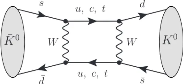
With these caveats in mind, it is useful to get a more quantitative idea of the severity of NP bounds from FCNCs FCNC constraints on the i. To this end, the Lagrangian (1.7) may be applied to transitions
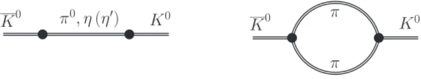
where a given flavor changes by two units between the initial and the final state, the so-called F = 2 processes. Within the SM, these processes are mediated by box diagrams like the one depicted in fig. 1, and are loop-, CKM-, and p2/M2
W-suppressed. In principle there is also a
GIM suppression, because two different quarks qi and qj in a given internal line amount to a
dependence of the kind m2
i≠ m2j, as already noted, hence to a partial cancellation. However,
this argument holds mostly for K0≠ ¯K0 mixing, whereas in the cases of B
d,s≠ ¯Bd,smixings,
the amplitude is totally dominated by the top-top contribution, hence there is basically no GIM cancellation at all.
K
0 s ¯ d¯
K
0 d ¯ s u, c, t u, c, t W WFigure 1: Example of a box diagram responsible
for ¯K0≠ K0 oscillations. One can obtain the case
of ¯Bd≠ Bd oscillations by the replacement s æ b. From the latter, one can obtain the case of ¯Bs≠Bs oscillations by the further replacement d æ s. Accurate data exist to constrain F = 2
amplitudes: the measurements of mass split-tings between the mass eigenstates of the K0 ≠ ¯K0 and the Bd,s ≠ ¯Bd,s systems, as
well as CP violation, quantified by ‘K for
the K0≠ ¯K0 system, and by sin 2—
(s) for the Bd(s)≠ ¯Bd(s) systems. Full details on the analyses as well as updated bounds can be found in [32–34]. To make an explicit ex-ample, one may consider the case of a shift to just the F = 2 operator allowed within the SM, namely13
L F=2 =ÿ
i”=j cij
2( ¯QLi“µQLj)2 , (1.8)
where the indices i, j label the external states: sd, bd and bs for K0≠ ¯K0, B
d≠ ¯Bd and
Bs ≠ ¯Bs respectively. From the (rather conservative) requirement that the new-physics
amplitude does not exceed in magnitude the SM one, |A F=2
NP | < |ASMF=2|, one arrives at constraints as severe as [33] > 4.4 TeV |Vú tiVtj|/|cij|1/2 ≥ Y _ _ ] _ _ [ 1.3 ◊ 104 TeV ◊ |c sd|1/2 5.1 ◊ 102 TeV ◊ |c bd|1/2 1.1 ◊ 102 TeV ◊ |c bs|1/2 . (1.9)
The by far strongest bounds are those from the K0≠ ¯K0 system, that therefore is generically regarded as the most sensitive probe of non-SM contributions. As anticipated above, these
12 An alternative approach consists in taking an explicit extension of the SM, whereby the extra d.o.f. and
their dynamics are completely specified. This approach is generally more predictive, because the short-distance couplings ciare in principle computable, but conclusions are model-specific.
bounds depend on the magnitude assumed for the Wilson coefficients. Given the very non-generic structure of the SM flavor violation, there is no reason to assume that the same structure holds also beyond the SM. Therefore, a natural choice seems to be to take the new-physics Wilson coefficients of O(1). In this case however, according to the bounds in eq. (1.9), flavor-violating new physics is allowed only way above the TeV scale – in particular, from the K0≠ ¯K0 system it is allowed at scales not lower than 10000 TeV. This circumstance is known as the flavor problem: if we insist that beyond-SM flavor effects should emerge at the TeV scale, then we have to conclude that the underlying new physics possesses a highly non-generic flavor structure [33].
Several ways have been put forward to circumvent the flavor problem. The most drastic one MFV is perhaps that of invoking minimal flavor violation (MFV).14 The latter is the assumption
that the SM sources of flavor breaking, in the quark sector the Yu and Yd matrices, are the
only sources of flavor breaking also beyond the SM.15 This assumption can be implemented
in the effective Lagrangian in eq. (1.7) via the following steps:
1. Identify the ‘flavor group’, namely the group of global transformations that the Yukawa couplings break. In the absence of Yukawa interactions (1.4), the gauge Lagrangian enjoys symmetry under a group of unitary transformations as large as GF © U(3)QL◊
U(3)uR◊ U(3)dR◊ U(3)LL◊ U(3)eR, where the subscript indicates the fermion field on
which the symmetry acts. This group is broken completely by the Yukawa interactions, apart from three U(1)’s, that can be identified with baryon number, lepton number, and hypercharge [35]. The part of this group relevant to quark flavor physics is Gq©
SU(3)QL◊ SU(3)uR◊ SU(3)dR.
2. Attribute to the SM Yukawa couplings formal transformation properties under Gq,
so as to recover invariance of Yukawa interactions under this group. By looking at interactions (1.4), one immediately sees that formal Gq invariance is recovered for Yu,d
transforming as Yu ≥ (3, ¯3, 1) and Yd≥ (3, 1, ¯3).
3. Accordingly identify the transformation properties required to any beyond-SM flavor structure in eq. (1.7), for the corresponding interaction to recover formal invariance under Gq. Then express this flavor structure in terms of Yu and Yd, as mentioned the
only Gq-breaking sources within MFV.
This procedure is justified to the extent that the scale of flavor breaking is well above the largest of the new-physics cutoffs in eq. (1.7). In these circumstances, expansions of beyond-SM flavor structures in terms of Yu,d are stable under RGE evolution. From the above
definition, it is clear that MFV is not a theory of flavor, since it takes the Yukawa couplings as given, without attempting any dynamical explanation of their structure. It is rather a criterion to achieve maximal protection of FCNC processes from beyond-SM contributions. The maximality is due to the fact that any new-physics flavor structure is assumed to inherit completely from the SM flavor structures, the Yukawa couplings. In this way, both the SM flavor-suppressing mechanisms, namely that of the CKM hierarchies and that of the quark mass patterns, are carried over to the new-physics interactions. This explains why the MFV solution to the flavor problem was denoted above as a drastic one. As a matter of fact, assuming that the cij couplings in eq. (1.9) are MFV, the new-physics scale goes down to
about 4 TeV.
14 I will follow here the effective-theory approach to MFV of [35]. The notion of MFV is also used to denote
CKM-like flavor violation in [36]. This definition is more restrictive than the one in [35], because, as also discussed in sec. 1.4, the peculiar form of the CKM matrix is only one of the mechanisms behind the pattern of SM flavor breaking, the other mechanism being the peculiar values of quark masses.
To summarize, MFV should not be regarded as ‘the expected pattern of beyond-SM flavor effects’, but rather as a useful way to ‘parameterize’ the question whether or not there are other sources of flavor-symmetry breaking at testable energies, beside the Yukawa couplings and the neutrino mass matrix. It should be stated clearly that, at present, the accuracy of this test does not exceed about 15% for MFV beyond-SM effects in K physics and about 25% in the case of B physics [32]. Therefore, we are still far from being able to claim that this hypothesis has been tested with high accuracy. Data on new FCNC observables and higher accuracies on existing observables, typically in the 1% – 10% range [33], are necessary to obtain bounds on beyond-SM effects able to exceed in severity those from electroweak precision observables, or else to finally uncover new effects.
1.6 Why pursuing flavor physics
Several of the points made in secs. 1.4 and 1.5 provide as many motivations for pursuing flavor physics. These motivations can be summarized by the following statements. Flavor observables provide an unequalled probe into higher energies and into the structure of in-teractions at these energies. Unequalled because beyond-SM flavor structures are plausibly different than the SM ones, hence it is correspondingly plausible that the SM pattern of flavor effects should be distorted by new physics, however high the scale at which it sets in. Furthermore several flavor observables can be measured with high accuracy. In short, the flavor-physics chances to unveil the unexpected rely:
• on the plausibility of new-physics effects showing up there; • on the richness of observables;
• and on the accuracy achievable in their measurement.
As an example, the race towards an ever more accurate knowledge of the CKM parame-ters, started with B-factories and still ongoing with the Belle upgrade, is not intended for precision’s sake, but rather because it is a very delicate SM consistency check, that will fail very easily in presence of new flavor-breaking interactions, even if their energy scale is not-so-nearby.
Given the progressive shrinkage of arguments about new physics having to show up at the EW scale, the possibility of new discoveries will depend more and more on experimental probes being able to test higher and higher scales. In this situation, flavor observables will have more and more weight in defining future strategies, bearing in mind also the definitely lower cost of measuring low-energy, high-intensity observables that probe a certain energy scale, with respect to producing collisions at that energy scale, assuming that this is doable at all.
Discoveries at stake are as formidable as the effort needed to hopefully make them reality. While ‘hopefully’ understates the possibility of failure, it should be stressed that drawing definite negative conclusions based on 20% tests is overhasty. This point can be made more explicit by one last example from history.16 The early 60s saw, as discussed above, a
flourishing of experimental tests of discrete symmetries, among the others the CP symmetry in the K0 ≠ ¯K0 system. The latter system consists of two mass eigenstates, denoted K
S
(shorter-lived) and KL (longer-lived). If CP is a good symmetry, then the KS is exactly CP
even, and cannot decay into 3fi, whereas the KLis exactly CP odd, and cannot decay into 2fi.
A dedicated search was carried out in Dubna by the group of E. Okonov, collecting about 600
16 The example to follow is quoted from the talk “Spacetime and vacuum as seen from Moscow”, given by
decays of KL to charged particles, and not finding a single KL æ fi+fi≠ candidate [38]. At
that stage, the lab administration decided to put an end to the search. Shortly afterwards, in 1964, this CP-violating decay was discovered at the level of 1/350 by the famous Brookhaven experiment of Christensen, Cronin, Fitch and Turlay [39], that was awarded the Nobel prize. This bold result decreed the breaking of a ‘sacred’17discrete symmetry, breaking that would
soon be recognised by Sakharov [41] as one of the conditions for the observed imbalance between matter and antimatter in the universe.
1.7 Content of the manuscript
The present manuscript is based on work I pursued in the years 2008 - 2013, on improving the Standard Model prediction of two among the flavor-physics observables that are deemed as most promising for beyond-SM effects. The latter include: (1) ‘K, that quantifies indirect
CP violation in the K0≠ ¯K0system, and (2) the very rare decay B
sæ µµ, recently measured
at the LHC. Item (1) will be dealt with in chapter2, where I will describe our reconsideration of the long-distance contributions to ‘K [1–3] and their impact on the follow-up literature.
Item (2) will instead be the topic of chapter 3. Here I will give an account of various systematic effects, discussed in [42], and affecting the SM branching ratio for Bs æ µµ at
the 10% level. Chapter3further describes the several aspects of the Bd,sæ µµ constraining
power, including in particular an effective-theory comparison between Bsæ µµ and Z-peak
observables [5]. Finally, the outlook part, chapter4, describes some further developments on the above subjects, and what is the progress to be expected on these and related observables.
17 L.D. Landau put forward in 1956 the idea of absolute CP invariance, namely the idea that the observed
‘sin’ of P-violation was committed by particles and antiparticles in a way to globally leave CP as a good symmetry [40]. This idea was widely accepted.
2 Indirect CP violation in the K
0≠ ¯
K
0system
Aim of the present chapter is to present a reappraisal of the long-distance contributions to ‘K, that quantifies indirect CP violation in the K0 ≠ ¯K0 system. This reappraisal was
undertaken in refs. [1–3]. The initial aim of ref. [1] was actually a reconsideration of the consistency between indirect CP violation in the K0- vs. the B
d-meson system, at the time
motivated by various tensions between data and theory predictions relevant to CKM-matrix fits. By a closer look at the level of precision required for this test to be meaningful, we almost stumbled on the necessity to reliably calculate and include the long-distance corrections to ‘K, in the following referred to as the multiplicative factor Ÿ‘. At the time of its proposal, the
Ÿ‘ factor made the above mentioned tensions worse, and indicated a clear pattern of
beyond-SM effects. This circumstance spurred further work on CKM fits, beyond-beyond-SM flavor effects, and associated model building. The latter aspect has lately lost momentum, especially because, at present accuracies, the initial tensions have by and large disappeared (and direct searches have likewise reported negative results so far). Mature data from LHCb and new data from the Belle upgrade will put a definite word on this issue, or maybe uncover effects at present swamped by too large errors. Independently of these tensions, a new, effective-theory calculation of the mentioned long-distance contributions to ‘K, and a systematic discussion
of this calculation and its limitations, is the lasting result of [1–3]. This result has motivated a new campaign of first-principle, non-perturbative calculations of the Ÿ‘ corrections within
lattice QCD, and with Ÿ‘of a number of historically challenging quantities related to K æ fifi
matrix elements.
2.1 Introduction to the problem
The discussion in this chapter is concerned with CP violation within the SM. More specif-ically, it is concerned with indirect CP violation, that namely does not arise directly from a decay, and is correspondingly denoted as direct CP violation [26]. Among the observ-ables that give access to indirect CP violation (CPV), three are especially well measured and theoretically controlled, namely ‘K, quantifying CPV in K0≠ ¯K0mixing, and sin 2—(s),
quan-tifying CPV in the interference between decays with and without mixing, for the Bd(s)≠ ¯Bd(s)
systems, respectively. (Note that this kind of CPV is mixing- and not decay-induced, hence it still qualifies as indirect CPV.) All these quantities will be properly defined in due course. The main point to make here is that, within the SM, there is one single source of CPV, namely the single phase ” of the CKM matrix. Therefore, within the SM, these three ob-servables are correlated to one another. Said otherwise, once one of them is measured, the other ones can be univocally predicted. Therefore, these three quantities offer a stringent test of the SM mechanism of CPV.
To make the discussion more concrete, let us focus on ‘K vs. sin 2—. As we will see later
on in the detailed derivation, the short-distance contributions to ‘K (from top-top exchange)
can be approximately expressed as
|‘K| ƒ C · ˆBK· sin 2— . (2.1)
Here C denotes a calculable coefficient and ˆBK a non-perturbative matrix element, input
from lattice QCD. The precise definition of these two quantities is not relevant here, and it will be dwelled upon in the detailed discussion. Eq. (2.1) neglects the subdominant short-distance contributions from top-charm and charm-charm exchange, that are likewise irrelevant for the point to be made here. This point is that there is a correlation, in particular a direct proportionality, as displayed in eq. (2.1), between indirect CPV in the K0-system
and the one in the Bd-system. This correlation can be understood intuitively by just noting
that, by its very definition – an observable quantifying CPV in K0≠ ¯K0 mixing – ‘
K must be of the form ‘K ≥ Im Q c aK¯0 K0 R d b . (2.2)
The imaginary part of the CKM couplings at the four vertices yields the sin 2— factor; the effective-operator structure arising from the diagram, calculated between the external ¯K0, K0 states, yields ˆBK; the rest is a calculable coefficient.
The novelty of [1] was, as mentioned, the reconsideration of various additional contribu-tions, especially long-distance ones, neglected in the previous literature in view of what used to be a large error on ˆBK. These contributions can be simplistically visualized as a negative
correction, of order ≠8%, to the r.h.s. of eq. (2.1), that would then become
|‘K| ƒ C · (1 ≠ O(8%)) · ˆBK· sin 2— . (2.3)
Now, taking sin 2— = SÂKS ƒ 0.68 (values refer to experimental averages at the time of
[1]), one obtained |‘K| = 1.78 ◊ 10≠3, to be compared with the experimental figure of
|‘K|exp = 2.232(7)◊10≠3. Conversely, identifying the l.h.s. of eq. (2.3) with its experimental
value results in sin 2— ≥ 0.8, too large with respect to the experimental average. Leaving aside errors for the moment being, in either case the discrepancy between central values is as large as 20%.
The above considerations will be made more quantitative in the next sections. 2.2 CPV in K physics: theory vs. experiment
In this section we introduce the minimal necessary formalism, and establish a contact between what experiment measures and what theory calculates. The K0≠ ¯K0 system consists of two flavor eigenstates, with flavor content
|K0Í ≥ A d ¯s B , | ¯K0Í ≥ A ¯ d s B . (2.4)
The CP symmetry acts on these states as follows
CP|K0Í = ei›| ¯K0Í ,
CP| ¯K0Í = e≠i›|K0Í , (2.5)
namely it connects them to one another, up to a phase that remains arbitrary, because the two states do not communicate via strong interactions. In the CKM conventions, where all CPV arises from the CKM phase ”, one can take
CP|K0Í = | ¯K0Í ,
CP| ¯K0Í = |K0Í , (2.6)
whence the two CP eigenstates are found to be |K±Í = |K
0Í ± | ¯K0Í
Ô2 , (2.7)
with namely CP-eigenvalues ±1, respectively. If CP were a good symmetry of the weak Hamiltonian HW, i.e. [CP, HW] = 0, then |K±Í would also be good physical eigenstates. As
we know after ref. [39], CP is slightly, but surely violated by weak interactions. Therefore the physical eigenstates are mostly the CP eigenstates, but for a small admixture with the opposite-CP state, namely
|KS,LÍ Ã |K±Í + ¯‘|KûÍ (2.8)
with |¯‘| π 1. Therefore, the shorter-lived |KSÍ state decays mostly into 2fi, and occasionally
into 3fi, and the other way around occurs for the longer-lived |KLÍ state.
To quantify the amount of CPV we need to connect what theory calculates with what experiment measures. Experiment can access the ratios
÷+≠© Èfi +fi≠|KLÍ Èfi+fi≠|KSÍ , ÷00© Èfi0fi0|KLÍ Èfi0fi0|KSÍ . (2.9)
These ratios would be zero if CP were conserved. From eqs. (2.8)-(2.9), CPV can occur either because of the small |K≠(+)Í component in the |KS(L)Í, that then decays into 3fi (2fi),
or because the |K±Í components of either physical eigenstate decay directly into the wrong-CP final state, 3fi or 2fi respectively. In the former case one has indirect wrong-CPV, through mixing; in the latter case CPV occurs directly in the decay. The two CPV components are therefore intertwined within the observables ÷+≠, ÷00.
In order to separate direct vs. indirect CPV components in the ÷+≠, ÷00 observables, we need to introduce final states of definite isospin SU(2)I. In fact, there is no direct CPV
in K æ (fifi)I.18 To obtain final states with definite isospin, one starts from recalling that
the u, d quarks are +, ≠ states, respectively, under isospin, and that, because of their quark content [26], the |fi+Í, |fi0Í, |fi≠Í states form an I = 1 triplet. |fifiÍ isospin eigenstates are accordingly obtained by composing symmetrically two I = 1 representations. In the PDG phase conventions one obtains
|fi+fi≠Í = Ú2 3|(fifi)0Í + Ú1 3|(fifi)2Í , |fi0fi0Í = Ú1 3|(fifi)0Í ≠ Ú2 3|(fifi)2Í , (2.10)
which are the relations we need in order to express measured states in terms of states of definite isospin. Plugging the first of these relations into eq. (2.9) yields
÷+≠ = aL,0+ 1 Ô2aL,2 aS,0+Ô21 aS,2 = ‘+Ô21 ‘2 1 + 1 Ô2Ê , (2.11) where ai,I © È(fifi)I|HW|KiÍ , (2.12)
and in the last member we have introduced the three amplitude ratios (all three of them small in magnitude) ‘K © aL,0 aS,0 , ‘2 © aL,2 aS,0 , Ê© aS,2 aS,0 . (2.13)
The ratio Ê = 0.045 is very well measured, and quantifies what is known as the I = 1/2 rule [44], namely the unexpected fact that in K æ fifi decays the final state is ≥ 1/Ê2 times more likely to be an I = 0 eigenstate than an I = 2 one. There is to date no simply
18 A beautiful discussion of this matter can be found in [43]. The main point is however that the I = 0, 2
amplitudes are fully described by just two strong phases. This in turn follows from the fact that, in QCD, a fifi state can only rescatter into itself (due to CP conservation, or else to energy conservation), and the isospin symmetry is almost exact.
understandable dynamical explanation of this fact, that remains one of the longest-standing puzzles in particle physics phenomenology. A numerical understanding starts to emerge from lattice QCD simulations (see in particular [45]) – this undertaking being per se extremely challenging, because, for one thing, the possibility to simulate the physical region of matrix elements with more than one hadron in the final state is limited by a no-go theorem [46], from which one has to find very clever workarounds.
The amplitude ratio in eq. (2.13) denoted as ‘K quantifies, as mentioned, indirect CPV in
Kdecays, and is our main quantity of interest. (It is the only ratio involving final states with the same isospin, so there cannot be direct CPV, as argued above.) Another combination of K æ fifi amplitudes, that we do not need to introduce here, accounts for ‘Õ, the parameter quantifying direct CPV in K decays. Through the definitions in eq. (2.13) the direct- vs. indirect-CPV contributions to ÷+≠, ÷00 are thereby disentangled.
2.3 Derivation of the ‘K formula
Let us now focus on
‘K © È(fifi)0|HW|KLÍ
È(fifi)0|HW|KSÍ
, (2.14)
as in eq. (2.13). We can express the |KS,LÍ states in terms of the |
(–)
K0Í ones by combining eqs. (2.7) and (2.8), yielding
|KS,LÍ = N¯‘
Ë
(1 + ¯‘) |K0Í ± (1 ≠ ¯‘) | ¯K0ÍÈ , (2.15) where N¯‘ is a normalization factor. We finally need symbols for weak matrix elements between |(–)
K0Í states and È(fifi)I| ones:
È(fifi)I|HW|K0Í © aIei”I ,
È(fifi)I|HW| ¯K0Í © aúIei”I , (2.16)
where aIdenotes a weak, complex amplitude, and ”Ia strong phase, accounting for final-state
interactions.19 Plugging eqs. (2.15) and (2.16) into eq. (2.14) gives
‘K = 1 + i ¯‘› ƒ¯‘+ i › ¯‘+ i › , with › © Im aRe a0
0 (2.17)
where the approximation on the r.h.s. of the ‘K equation is well justified, given that both
of ¯‘ and › are small in magnitude. Eq. (2.17) is a first important formula on ‘K, and it
is worthwhile to pause on its physics content. This relation shows that ‘K is the sum of
two contributions: the first, ¯‘, is due to the fact that the weak Hamiltonian mixes different CP eigenstates (see eq. (2.8)), it represents the main contribution, and is fully calculable in perturbation theory;20 the second, i›, is due to the small but non-zero weak phase of the
K0 æ (fifi)0 amplitude, and represents a subdominant correction. Its non-negligibility in view of the improved errors on the rest of the ‘K parametrics was one of the points made
originally in [1].
The › correction is not easy to estimate accurately. A first strategy was proposed in [1] (see also related work by U. Nierste in the Fermilab report [43]), whereby this correction is extracted from data on ‘Õ/‘
K; a more refined effective-field theory treatment was performed
19 That this final-state interaction can only be elastic and is thus fully described by just two scattering phases
follows from kinematics and QCD conservation laws, and is known as Watson’s theorem [47].

![Table 1: Input parameters used in ref. [4] for the determination of B (0) s,SM and B (0) d,SM](https://thumb-eu.123doks.com/thumbv2/123doknet/14451839.711040/45.892.222.670.127.301/table-input-parameters-used-ref-determination-sm-sm.webp)