Anomaly Detection in Cloud Applications

(1)

HAL Id: hal-01406168

https://hal.laas.fr/hal-01406168

Submitted on 30 Nov 2016

HAL is a multi-disciplinary open access archive for the deposit and dissemination of sci-entific research documents, whether they are pub-lished or not. The documents may come from teaching and research institutions in France or

L’archive ouverte pluridisciplinaire HAL, est destinée au dépôt et à la diffusion de documents scientifiques de niveau recherche, publiés ou non, émanant des établissements d’enseignement et de recherche français ou étrangers, des laboratoires

Anomaly Detection in Cloud Applications

Javier Alcaraz, Mohamed Kaâniche, Carla Sauvanaud

To cite this version:

Javier Alcaraz, Mohamed Kaâniche, Carla Sauvanaud. Anomaly Detection in Cloud Applications: Internship Report . Machine Learning [cs.LG]. 2016. �hal-01406168�

(2)

Internship Report

Anomaly Detection in Cloud Applications

Javier Alcaraz

L3 Économie et Mathématiques

Université Toulouse 1 Capitole

Laboratoire d’Analyse et d’Architecture des Systèmes

LAAS-CNRS

Toulouse, France

Internship supervisor : Dr. Mohamed Kaâniche

Co-supervisor : PhD candidate Carla Sauvanaud

17th _{May - 22}nd _{July 2016}

Key Words: Anomaly detection, virtual machine, system monitoring, machine learning, ensemble learning, principal component analysis, random forest, precision, recall, mixture model, time series.

(3)

Acknowledgements

This internship at LAAS-CNRS has been an excellent opportunity for me to learn many things and be in contact with the research world. Therefore I would like to thank the people who have contributed towards making this internship possible.

Firstly, I would like to thank my internship supervisor, Dr. Mohamed Kaâniche, Research Director at LAAS-CNRS, for his trust and confidence in me as well as the guidance during this internship.

Then, I would like to thank especially my co-supervisor Carla Sauvanaud, PhD candidate at LAAS-CNRS, for providing the subject of this internship, and for the countless hours she spent helping me conduct this study.

My gratitude also goes to Dr. Karama Kanoun, Research Director at LAAS-CNRS, for her support and useful suggestions which have been in-cluded in this work.

Finally, many thanks to Cédric Allain, one of my classmates at Toulouse School of Economics, as without his help I would not have found this in-ternship.

(4)

Internship search and choice of subject

I started searching for an internship in November 2015, roughly around the date of the Business Networking Day (BND) at TSE. I had been told that the BND was a good experience for undergraduates, but that it was really meant for master students and it would be unlikely for me to find an internship there. However, I spoke to several representatives of partner companies who assured me that it was possible for third year students to apply for the internships they offered. I therefore completed two application forms for different companies but was quickly out of the selection process so I assumed that my chances were not good with the other firms either.

It was then that I started looking for an internship more independently, using the Alumni website from TSE and some contacts in Spain. I was rather disappointed when I realised that most of the internship offers at the Alumni website were also for master students, and I only managed to send an application email to a firm in the energy sector, but they told me the position was no longer available.

Finally, I had just found a possibility in a local firm from my home town in Spain when a fellow student told me about this internship at LAAS-CNRS. I found that this would be much more interesting and useful than what I could have done at my home town, so I finally did not apply for the position in Spain.

(5)

General working conditions

My internship took place at the Laboratory of Analysis and Architecture of Systems (LAAS), which is a CNRS research unit, located near the Paul Sabatier University campus in Toulouse. In paricular, I worked at the De-pendable Computing and Fault Tolerance (TSF) team, which studies the dependability of computing systems.

The working conditions at TSF were excellent, as a big multipurpose room is available for interns to use. I was therefore assigned to a personal computer I used during the entire internship, running Ubuntu 14.04 and all necessary open-source software, such as R, python and LaTeX which I have used throughout the internship. Furthermore, the environment at TSF was friendly and welcoming from the first day.

Finally, my particular task consisted in trying to find an alternative way of detecting anomalies in a cloud application in the context of Carla Sauvanaud’s PhD thesis, as will be later explained in more detail. As a re-sult, my task was rather unbounded and independent, although many clar-ifications were necessary so discussions were frequent. For example, when I experienced some difficulties understanding specific vocabulary at the be-ginning of my internship.

(6)

Report summary

In this section I will explain the objective of this internship, the strategy I adopted and I will give a brief overview of the results that will follow.

In very general terms, my internship consisted in analysing data from several experiments [10] on the evolution of a virtual network over time. Using the available data, the objective was to develop a program which could perform online anomaly detection on virtual networks.

The available data for this study consists of tables containing informa-tion regarding several virtual machines (i.e. the system) which are moni-tored every 15 seconds. Two sources of data are available: the first source provides data with 150 variables, and the second source with 250. In any case this number of variables is considered as high-dimensional. In addition, a qualitative variable classifies every entry into several possible categories, according to the state of the system, which is either exhibiting normal or anomalous behaviours.

In statistical terms, the problem we deal with in this work implies cre-ating a certain decision rule based on the data collected to be able to (accu-rately) forecast the state of the system (the value of the qualitative variable) knowing the value of the other variables. Therefore this is a classification problem.

At first I thought about the possibility of applying techniques I already knew from my bachelor studies. Those range from descriptive statistics to more sophisticated techniques such as cluster analysis and principal com-ponent analysis. However, it was clear that descriptive statistics would be of little use here, and cluster analysis had already been tested during Carla Sauvanaud’s PhD thesis [11] with results that were not promising compared to other techniques.

Therefore it soon became clear that principal component analysis was the only tool I could use and that I would have to learn new techniques currently in use. The algorithm I used the most is random forest.

Using mainly these two tools, and sometimes other tools described later, I tried to solve this classification problem in many different cases depending on the source of the data and the precision of the fault detection, i.e. the number of categories. As the reader will see, the report shows how principal component analysis does not help anomaly detection in this case and random forest generally obtains the best results.

(7)

Index

1 Abbreviations and acronyms 8

2 Tables and figures 9

3 Preliminary chapter 11

4 Introduction 12

5 Detection approach 14

5.1 Detection objectives and classification problem . . . 14

5.2 Monitoring . . . 16

5.3 Feature selection approach . . . 17

5.4 Validation metrics . . . 19

6 Detection results of SLA violations 20 6.1 Results with data from grey-box monitoring . . . 21

6.2 Results with data from black-box monitoring . . . 25

6.3 Results with data from both monitoring sources . . . 27

7 Detection results of errors 28 7.1 Results with data from grey-box monitoring . . . 28

7.3 Results of detection with component localisation . . . 29

8 Sensitivity analysis of the Random Forest algorithm 29 8.1 Maximum number of nodes . . . 30

8.2 Number of trees . . . 31

9 Other methods 33 9.1 Detection with time series . . . 33

9.2 Detection with gaussian mixture models . . . 34

(8)

1 Abbreviations and acronyms

Acronyms

AUC Area Under the Curve BCP Bayesian Change Point

CSP Communications Service Provider FPR False Positive Rate

GMM Gaussian Mixture Models PCA Principal Component Analysis PSR Percentage of Successful Requests PUR Percentage of Unsuccessful Requests ROC Receiver Operating Characteristic SLA Service-Level Agreement

SLAV Service-Level Agreement Violation TPR True Positive Rate

VM Virtual Machine

(9)

2 Tables and figures

List of Tables

1 Benchmark prediction results of SLAV: all detection-VMs, detection with root cause localization, grey-box. . . 14 2 ROC AUC for all metrics with 64 trees, grey-box . . . 21 3 Predictions of SLAV: all metrics versus single VM, detection

with root cause localisation, grey-box. . . 22 4 Predictions of SLAV: all metrics with PCA, detection with

root cause localisation, grey-box. . . 23 5 AUC for PCA with 12 components and 50 trees, grey-box . . 23 6 Predictions of SLAV: PCA on Bono, detection with root cause

localisation, grey-box. . . 24 7 Predictions of SLAV: PCA on Sprout, detection with root

cause localisation, grey-box. . . 25 8 Predictions of SLAV: PCA on Homestead, detection with root

cause localisation, grey-box. . . 25 9 AUC for all metrics with 64 trees, black-box . . . 26 10 Predictions of SLAV: all metrics versus single VM, detection

with root cause localisation, black-box. . . 26 11 AUC for PCA with 50 trees, black-box . . . 27 12 Predictions of SLAV with different variables: all vms, 1064

trees, detection with root cause localisation, grey-box and black-box. . . 28 13 AUC for error detection: all metrics with 64 trees, black-box 29 14 ROC AUC for errors detection with component localisation:

all metrics with 1064 trees . . . 30 15 Predictions of SLAV with different number of nodes: all vms,

50 trees, detection with root cause localisation, grey-box. . . 31 16 AUC for all metrics with different number of trees, grey-box . 31 17 Predictions of SLAV: all metrics combined, detection with

root cause localisation, grey-box. . . 32 18 Predictions of SLAV: all metrics combined, detection with

root cause localisation, grey-box. . . 33 19 Predictions of SLAV with BCP: PCA components, binary

detection, grey-box. . . 33 20 Predictions of SLAV with BCP: original variables, binary

(10)

List of Figures

1 Monitoring sources . . . 16 2 Per-VM approach. . . 17 3 Joint approach. . . 18

(11)

3 Preliminary chapter

This internship took place at the Laboratory of Analysis and Architecture of Systems (LAAS), one of the research units of the National Center for Scientific Research (CNRS). The CNRS is a public organisation which de-pends on the Ministry of Education and Research and was founded in 1939. Its missions and research fields are very diverse, and the LAAS is part of the Institute for Engineering and Systems Sciences, one of the ten research institutes of the CNRS.

In particular, the laboratory is one of the 34 institutes to hold the "Carnot" label, a distinction which proves the scientific excellence of its research as well as its socio-economic influence. In addition, LAAS is associated with all of the founding members of the University of Toulouse.

Research at LAAS is in turn subdivided into eight different departments, which cover different fields such as Energy Management or Robotics, for example. I worked at the research team on Dependable Computing and Fault Tolerance (TSF), which is part of the Crucial Computing department, which deals with dependability and resilience issues in computing.

In particular, TSF is specialised in analysing the ways to maintain the dependability of complex systems that evolve over time and are subject to accidental as well as malicious faults. A general overview and many important definitions of this research area were given in a famous paper [2] which has been very useful for me during this internship.

The report that will follow has been written during this internship and is intended to constitute an organised summary of my work at LAAS and the results I found. I have tried to keep its structure close to that of a research article, which is why I have used LaTeX throughout this internship.

(12)

4 Introduction

Virtualisation is a computing method that enables by software means to run several machine instances on a single hardware. The machines are called

Virtual Machines (VMs) and are potentially different to each other in that

they rely on different operating systems. The VMs instructions to access the hardware resources (CPU, memory, etc) are interpreted and filtered by a single entity called the Virtual Machine Monitor or hypervisor. The hypervisor shares the underlying resources between each of the VMs. Cloud computing is a marketing paradigm that makes use of virtualisation. As grid computing, it uses virtualised servers so as to reduce deployment costs of applications. Indeed, virtualisation enables several users to access all types of services potentially deployed on the same server. In other words, users can share hardware in the case their applications do not fully use all resources. Clouds then make the service available on demand and through the Internet.

As new services arise from the cloud paradigm, we particularly focus our work on the network functions (such as routers, or firewalls) that are mi-grated to cloud commodity servers. These functions are usually deployed on specialised hardware (like CISCO) made for the purposes and stringent requirements of the network functions. Telecommunication operators in-tend to make the best out of clouds and deploy several network functions on virtualised cloud commodity servers. They are called Virtual Network

Functions (VNF).

As it is a new concept, VNF are still to be improved, especially consider-ing their dependability. In this document, we more particularly work on the fault tolerance mechanisms of VNF through the task of detecting anomalies in them.

Anomaly detection is an important problem that has been widely stud-ied in several domains and often tackled with machine learning approaches [3][6][5][12][1][7]. Our goal is to explore the ability of such methods to ac-curately detect anomalies in VNF. The datasets used are the monitoring data (CPU consumption, memory consumption...) collected from a sim-ple VNF platform deployed at LAAS CNRS by Carla Sauvanaud. The datasets were collected as anomalies were injected into the VNF VM at reg-ular time steps. Also, heavy workload peeks were injected. The datasets are labeled, meaning that each entry is labeled as corresponding to a time during which an anomaly happened or not. We use data collected from three VMs called Bono, Sprout, and Homestead. Data collection was performed over five days. Data was collected from two different monitoring sources during the same time period: a grey-box monitoring source (the operating system of the VNF VMs is required for the monitoring to be executed) and

(13)

a black-box monitoring source (no knowledge of the VNF is required). Carla Sauvanaud’s PhD thesis work (from now on referred to as the "thesis study") uses these datasets by transforming them and using the Random Forest al-gorithm to detect anomalies in the VNF. The aim of this document is to exploit the same datasets by transforming them in different manners and using the transformed data to perform detection by means of the Random Forest algorithm and other machine learning methods. We also compare results obtained while using either one of the monitoring sources.

We more particularly compare the thesis results to the results obtained using the following methods:

1. Using the Principal Component Analysis (PCA) method to reduce the number of dimensions.

2. Assembling the data from the three virtual machines into one single dataset to increase the amount of information.

3. Performing a Bayesian Change Point detection in time series. 4. Performing a Gaussian mixture model.

Some of these methods are supervised as they require a training of the model on labeled data, and some of them are unsupervised and do not require the labels of the data to perform detection.

As a basis for comparison, table 1 shows the detection results while using the grey-box monitoring source. Results are presented depending on the input data of the algorithm and on the ability of the algorithm to detect anomalies while identifying the probable source of the anomaly (it corre-sponds to a multiclass classification problem). For instance, the detection from the data related to the Bono VM of anomalies happening in the Sprout VM and correctly identified as such, is 0.99 precision, 0.87 recall and 0.92 F1-score. Thus, several detections are performed.

Firstly, in section 5, we explain the detection approach used in this doc-ument. This consists of a definition of our case of study and a description of the four feature selection approaches used in this document. More pre-cisely, we apply the Random Forest algorithm to a dataset containing all the metrics of the three VMs. The idea behind this is that with more available data the algorithm should perform better for all predictions. The drawback is that interpretation is harder with so many variables. Then, we apply random forest to several datasets containing metrics from only one VM re-spectively. We also apply the PCA method to reduce the number of variables in an attempt to condense information from all three machines. Secondly,

(14)

Table 1: Benchmark prediction results of SLAV: all detection-VMs, detec-tion with root cause localizadetec-tion, grey-box.

Detection

Measure Cause in Cause in Cause in Cause by

input Bono Sprout Homestead heavy load

Precision 0.98 0.99 0.99 0.93 Bono Recall 0.86 0.87 0.83 0.94 F1-score 0.92 0.92 0.91 0.93 Precision 0.99 0.98 0.98 0.92 Sprout Recall 0.80 0.90 0.80 0.93 F1-score 0.89 0.94 0.88 0.92 Precision 0.99 0.99 0.96 0.90 Homestead Recall 0.79 0.85 0.83 0.94 F1-score 0.88 0.92 0.89 0.92 Ensemble Precision 0.99 0.98 0.99 0.92 analysis Recall 0.82 0.93 0.83 0.96 F1-score 0.90 0.95 0.89 0.94

in section 6 we present the results of detection depending on these feature selections. These detections are aimed at detecting service violations (slow service for customers). As we will see, results show that with more data the algorithm performs slightly better, and that satisfactory results can be obtained with only 10 dimensions on the PCA. However, some information is lost and these results are not optimal.

Thirdly, in section 7 we briefly present some results with detection of errors, which are preliminary symptoms of service violations. These results have proved to be better than those of service violations. Section 8 presents a sensitivity study of the random forest algorithm, before presenting detection with other methods in section 9 and finally concluding in section 10.

5 Detection approach

5.1 Detection objectives and classification problem

In this study we aim at detecting two types of anomalies in a system. The first type is the detection of the anomalous behaviours of the system, and the second type is the detection of service level violation. It is relevant to detect anomalous behaviours (or errors) because they can lead to potential degradation of the service level if they last in time or if they keep increasing in intensity. Detecting anomalous behaviours is a way to anticipate potential service level violation however some detection might not be relevant because

(15)

they would have never lead to service level violation. The detection of service level violations is another of our objectives which triggers alarms that should be taken into consideration extremely fast because the user potentially might be experiencing service degradation. The service level is evaluated as the percentage of successful completion of user requests by the system, in other terms, the percentage of successful requests (PSR). In our work, we evaluate the percentage of unsuccessful requests (P U R = 1 − P SR) to study system SLA violations. The SLA is satisfied as long as the PUR does not overpass a maximal PUR value called PUR_max, or the PSR is not below a minimum value. An SLA violation (SLAV ) happens when PUR_max is overpassed (P U R > P U R_max).

The detection of anomalous behaviors or SLAV can be handled as a binary classification task: is there an anomalous behaviour or not? And is there an SLAV or not?

Nonetheless, the detection with root cause localisation handled by means of multiclass classification is the preeminent detection investigated in this work. It performs detection with localisation of an anomalous behaviour cause, by assigning one class label to each anomalous behaviour depending on its localisation. In this work, we show results while localising anoma-lies causes with two different granularities: the VM granularity, and the component granularity. Considering the VM granularity, the cause of an anomalous behavior can be an anomalous VM suffering from local perfor-mance stressing, or it can also result from a global heavy workload toward the system. Considering the component granularity, the cause of an anoma-lous behavior is regarded as coming from either the CPU, memory, disk or network interface components.

Machine learning is a famous field of computer science aimed at getting automatic computing procedures to learn a task without it being explic-itly programmed. It turned out to be extremely relevant for classification problems [8]. Machine learning can be applied to our problem so as to clas-sify behaviors corresponding or leading to anomalies, or not. There are a plethora of machine learning algorithms and a lot of them are specifically dedicated to handle numerical data. Actually, monitoring data enables us to directly observe a system and represent its behaviours by means of numer-ical data. Representing a behaviour needs some heavy preprocessing when using audit data, OS logs, or application logs.

This work particularly focuses on the identification of anomalies from monitoring data of VMs OSs such as CPU consumption, disk I/O, and free memory.

With respect to the machine learning models that we aim to build for detection (in our case, classifiers), samples of labeled monitoring data are needed to train them to discern different system behaviours. Considering our two first objectives, samples should be labeled with two classes correspond-ing to normal or anomalous behavior so as to train models to classify these

(16)

two behaviors. As for the third objective, samples should be labeled with several classes according to the several SLA violation origins in the system. This method is called supervised learning (by opposition to unsupervised learning, i.e., clustering). Samples are called training data. They are ob-tained during a training-purposed runtime phase (i.e., training phase) during which a testbed or a development infrastructure is monitored while expe-riencing different types of behaviors. Based on our field knowledge about system anomalies that may lead to SLAVs, we can emulate them during a training phase and train models from the collected data. The emulation is performed through errors campaigns. Once a model is trained from a train-ing dataset, it can be used online durtrain-ing a detection phase (i.e. durtrain-ing the runtime of the system). Thereupon, it performs predictions of whether a given monitoring sample belongs to a particular class of behaviours that it learned to discern. The ability of models to perform accurate predictions is referred to as predictive ability in this study.

5.2 Monitoring

5.2.1 Definition

Monitoring provides units of information about a system that are called performance counters (referred to as counters). The actual counter values being collected from a system are called performance metrics (referred to as

metrics). A vector of metrics collected at a given timestamp corresponds to

a monitoring observation (also referred to as observation). 5.2.2 Monitoring sources

In this work, observations related to a system VMs hosted in a virtualized infrastructure are collected from two monitoring sources, namely the hyper-visor, or the OS of the VMs. They are described below and represented in Figure 1. App OS VM App OS VM App OS VM Hypervisor Monitoring via agents installed in OS Monitoring via hypervisor API Grey-box Black-box

Figure 1: Monitoring sources

• The hypervisor hosting the system VMs can provide monitoring data related to each VM it hosts such as the memory, the CPU speed or

(17)

the network bandwidth that the hypervisor grants to the VM. Such a monitoring source is called black-box as it does not need any tool to be installed in the VMs.

• Monitoring data can also be collected directly from the OS of the sys-tem VMs. Collected observations from VMs require the installation of monitoring agents in VMs. This is referred to as a grey-box monitoring source. Considering this source, the number of available counters is more important than in the case of the black-box source since they can relate to the OS performance in terms of system buffers size and use, and in terms of memory pages state for instance. These low level VMs counters cannot be known by the underlying hypervisor.

Both monitoring sources provide periodically observations related to each single VM of the system. We evaluate the benefits in terms of the predictive accuracy a grey-box monitoring may provide for the detection objectives. For both monitoring sources, our approach does not require knowledge about the system under study.

5.3 Feature selection approach

Having described the two monitoring sources, we now describe the methods used for feature selection. Several possibilities are investigated. Firstly, using only features from one virtual machine, which we call per virtual machine detection, secondly, using data from all virtual machines, which will be called the joint approach, and finally using principal components of a Principal Component Analysis on our original variables.

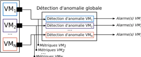
5.3.1 The per-VM approach

The per-VM approach consists in applying one anomaly detection task on subsets of the monitoring data according to the VM to which they are re-lated. It is represented in figure 2

Système

Détection d'anomalie globale

VM1 VM2 VMN Métriques VM1 Métriques VM2 Métriques VMN... ... Détection d'anomalie VM1 Détection d'anomalie VMN Détection d'anomalie VM2 ... Alarme(s) VM1 Alarme(s) VM2 Alarme(s) VM3

Figure 2: Per-VM approach.

For each of the two monitoring sources described, there are three moni-tored virtual machines for which data is available, called Bono, Sprout and Homestead. Once the datasets have been cleaned and the useless (constantly

(18)

equal to zero) variables removed, we have the following data available: for the grey-box source, we dispose of a dataset of 13126 observations and 118 features in the case of bono, 122 features for sprout and 120 features for Homestead; for the black-box source, the data available is composed of 6600 observations and 95 features for Bono, 98 features for Sprout and 94 features for Homestead.

5.3.2 The joint approach

The joint approach consists in applying one anomaly detection task on the entire monitoring data comprising monitoring from all the monitored VMs. It is represented in figure 3

Système

Détection d'anomalie globale

VM1 VM2 VMN Métriques VM1 Métriques VM2 Métriques VMN... ...

Détection d'anomalie : toutes VMs

+

concatenation Alarme(s) VM1_{ou VM2}

ou VM3

Figure 3: Joint approach.

The joint approach uses data from the three virtual machines, consider-ing data from one monitorconsider-ing source. This is easily feasible because data for the three virtual machines is collected at the same time, therefore the three data sets have the same number of observations, which are recorded at the same time. In this case, we have two datasets to test: for grey-box mon-itoring, it contains 13126 observations and 360 features, and for black-box monitoring it has 6600 observations and 287 variables.

5.3.3 Both sources approach

Finally, the last feature selection approach used in this study. It combines the data from both monitoring sources. Most of the data is actually re-dundant, but this is an insightful approach, as it allows the study to assess the relative importance of information collected by each of the monitoring sources, in order to decide which one should be used.

5.3.4 Principal Component Analysis

PCA is a statistical method that aims to reduce the amount of variables in a dataset by eliminating redundancies between them. The procedure to achieve this consists in an orthogonal transformation, which projects the observations to a new space where the variables (called principal compo-nents) are uncorrelated. In more detail, the first principal component is chosen as the linear combination of variables with the highest variance, and

(19)

the subsequent components are chosen in the same way with the additional constraint of zero covariance with the previous components. The number of principal components kept can be chosen, but is necessarily smaller than or equal to the number of variables. In general, many components are dis-carded because, by construction, the last components have small variance and therefore increase the size of the dataset without providing much addi-tional information.

The main interest of PCA is that it can considerably reduce the number of dimensions of a dataset. This can sometimes be very useful, especially when several variables are highly correlated, which leads to redundancy in the data studied. The idea behind this procedure is that we might achieve better results if we manage to concentrate the important information contained in the data in a smaller number of variables, which are called principal components. This PCA method will be used in all approaches described above. The important choice of the number of components to keep, which will be explained in further detail, leads to a number of different datasets to test for both monitoring sources.

5.4 Validation metrics

The validation of the machine learning models to classify anomalous behav-iors is based on the Receiver Operating Characteristic (ROC) curve, as well as the precision, recall and F1-score. ROC curves are obtained by computing performance measures for different thresholds of the prediction probabilities. The ROC curve corresponds to the true positive rate (TPR) against the false positive rate (FPR). A perfect classifier would have an area under the curve (AUC) of 1.

The ROC curves are relevant to study the predictive accuracy of our models and their consistency while the prediction probability thresholds change. They enable us to evaluate our approach with metrics that do not change with the proportion of normal or anomalous behaviors in the validation dataset. In other words, they are not sensitive to the class skew and the results can easily be generalized to several case scenarios of detection with different baseline distributions. Also, the FPR (i.e., the rate of false alarm) can easily be analysed and it is of interest in our domain. Indeed, it is expensive (in terms of time and money) for a system administrator to take counter measures on components, and the fewer false alarms there are, the better is the approach.

As for precision and recall, they are defined by the well known formulas:

P recision = _{T P +F P}T P and Recall = _{T P +F N}T P where T P are the true positives,

F P are the false positives, and F N are the false negatives. The F1-score

corresponds to the harmonic mean between precision and recall. These metrics provide a precise evaluation of the predictive accuracy, that can

(20)

give an account of the efficiency of our method for a CSP. They are defined with a given prediction probability threshold.

Precision, recall and F1-score metrics are provided for the description of experiments results for which they are more relevant for the sake of our discussion.

6 Detection results of SLA violations

In this section we perform detection on the data described above to detect Service Level Agreements (SLA) violations in the deployment of a case study presented in [10]. The three main entities on which we focus our work are a proxy named Bono, a router named Sprout, and a database named

Homestead. In order to evaluate whether our detection methods perform

good detection we put labels on each entry of the data depending on whether there was an SLAV during the recording of the entry or not. Labels are integers identifying the type of SLAV and its root cause. The label 0 means that there is no anomaly.

Given that our work on anomaly detection is ruled by two monitoring sources, two detection objectives and several levels of root cause localisation, (we either detect the root cause to be in one single VM or in one resource of a VM) our study has a lot of parameters and all combinations of parameters are not presented in this document. We particularly focus our work on the use of PCA and black-box monitoring data.

Detection results are presented throughout this section in the form of tables showing mainly ROC AUC (referred to as AUC) but also Precision and Recall, computed as we have explained previously. The reason for this choice is that our main purpose is comparing the effectiveness of the differ-ent approaches tested in this study. For comparative analysis, a table is the most concise and easily interpretable way of presenting our results. However, using Random Forest algorithm implies that it is possible to repeat the de-tection experiment and obtain different results by introducing randomness. This is why box plots constructed from, for example, 100 detection results, would be a more rigorous way of presenting results. However, in order to avoid making this report unnecessarily long, we will not present these box plots in this document. The reader may bear in mind that the conclusions drawn from the tables prevailed when analysing the box plots.

(21)

6.1 Results with data from grey-box monitoring

6.1.1 Joint approach

In this section we will show the results obtained with all metrics from the three virtual machines (named Bono, Sprout and Homestead). Intuitively, we expected that results would be higher than in the thesis study because there are more variables in the dataset. Results are shown in table 2 for 64 trees. Please refer to the sensitivity study on page 29 for a detailed explanation of this choice of number of trees.

Table 2: ROC AUC for all metrics with 64 trees, grey-box Number

of trees Bono Sprout Homestead heavy load

64 AUC 0.999 0.999 0.999 0.961

Precision 0.94 0.94 0.94 0.85

64 Recall 0.94 0.93 0.90 0.93

F1-score 0.94 0.93 0.92 0.89

As we can see in table 2, the results obtained seem better with all metrics combined. To confirm this, the results showing precision and recall for each fault type are also shown in the same table.

We can now compare these results to those obtained from the thesis study. It seems that these results are similar to those produced by the ensemble analysis method in the thesis study. This is an intuitive outcome given that in both cases the same data is used.

6.1.2 Per-VM detection: comparison of results

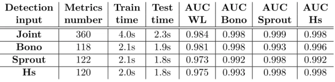
In this section we present the results of detection performed on data re-lated to each VM respectively. The aim is to compare the results obtained with those achieved with the joint approach, and record the computation times. Ultimately, this section should allow us to decide whether having more data can provide better detection results, in terms of the increase in predictive ability and/or computation time. Computation time and AUC are shown for 64 trees in table 3. These results enable us to compare both approaches.

These results show that predictive ability is improved for all SLAV with the joint approach. However computation time also increases with more

(22)

Table 3: Predictions of SLAV: all metrics versus single VM, detection with root cause localisation, grey-box.

Detection Metrics Train Test AUC AUC AUC AUC

input number time time WL Bono Sprout Hs

Joint 360 4.0s 2.3s 0.984 0.998 0.999 0.998

Bono 118 2.1s 1.9s 0.981 0.998 0.993 0.996

Sprout 122 2.1s 1.8s 0.973 0.992 0.998 0.992

Hs 120 2.0s 1.8s 0.975 0.993 0.998 0.998

variables. Nevertheless, training time only increases by a factor smaller than 2, and remains acceptable for our purposes. Taking into account that the model is probably going to be trained once a month, the training time with the joint approach is acceptable. In addition, testing time does not increase, which means that in the case of online detection (when the model is already trained and used during runtime) having a larger number of variables does not seem to slow down the algorithm. These results show that, in this case, all variables should be used.

6.1.3 Principal Component Analysis with Joint Approach

In this case, a PCA was performed on a dataset containing all grey-box metrics for the three virtual machines, having eliminated the metrics which are always equal to 0. The result is a dataset with 360 quantitative vari-ables and one qualitative variable which gives the class of each observation vector. The PCA is performed on the quantitative variables, and the results obtained have interesting interpretations.

The key choice here is to decide how many dimensions should be kept to be used for the detection. This depends on a tradeoff between accuracy and interpretability. However, there are several typical PCA criteria we can use to guide our choices. The first one is interpretability, which means that only the principal components which have interpretable associated groups of highly-correlated variables are kept. The second criterion is keeping all the principal components with a variance greater than 1. Finally, in line with our previous examples, it was chosen to maintain enough components to achieve a cumulative variance of 91%. Several tests were realised with different numbers of dimensions, for which the results are shown in table 4. These results show that PCA is not relevant in this case. Although the dimension reduction is efficient (from 360 metrics to as low as 10 in the case of the first line of table 4), some information is lost and results are

(23)

Table 4: Predictions of SLAV: all metrics with PCA, detection with root cause localisation, grey-box.

Detection

Precision 0.98 0.90 0.92 0.85 PCA 10 Recall 0.58 0.72 0.67 0.90 F1-score 0.73 0.80 0.78 0.87 Precision 0.98 0.88 0.90 0.85 PCA 12 Recall 0.59 0.73 0.72 0.88 F1-score 0.74 0.80 0.80 0.86 Precision 0.98 0.90 0.94 0.87 PCA 20 Recall 0.60 0.72 0.69 0.88 F1-score 0.75 0.80 0.80 0.87 Precision 1.00 0.90 0.92 0.86 PCA 30 Recall 0.58 0.73 0.68 0.85 F1-score 0.74 0.80 0.78 0.86 Precision 0.99 0.93 0.94 0.88 PCA 100 Recall 0.71 0.73 0.68 0.88 F1-score 0.82 0.82 0.79 0.88

somewhat lower than those obtained with all the dimensions. It does not seem possible to provide an acceptable prediction with only some variables, as F1-scores have dropped to around 0.75 with PCA compared to 0.9 in the thesis study. From the different number of dimensions tested, 100 is the best option if one seeks to maximise the algorithm’s performance. However, if the decision criterion is to ease the interpretation of results, 10 or 12 dimensions would be the best alternative considering that with a higher number of dimensions results are not interpretable. The AUC is shown in table 5 for the twelve-dimensional case.

Table 5: AUC for PCA with 12 components and 50 trees, grey-box Detection

(24)

We can see that results are not much better with 100 variables than with only 12 of them, which illustrates the power of PCA. Only a few components gather most of the information. Such results were not expected.

6.1.4 Principal Component Analysis with the per-VM approach In this section we investigate the results in terms of precision and recall when the PCA is used on data from one VM at a time. This approach has not yet been tested, and it is interesting to know which metrics will be assembled together in each principal component. Due to the bad results achieved by PCA in the case of the joint approach, this section seeks to determine whether the PCA is not suitable in this case or whether the problem relies on mixing data from all virtual machines.

Therefore a PCA was performed on each of the data sets from the three virtual machines. For this study, only grey-box metrics have been used, as PCA did not perform differently on these metrics than those from black-box monitoring. The parameters chosen for the random forest algorithm were the same we have used previously in PCA examples.

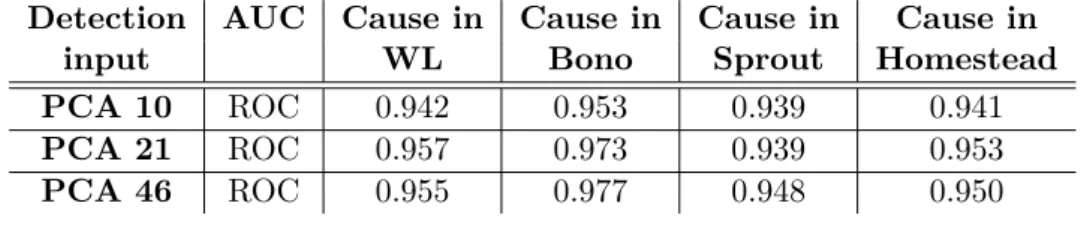
Results are shown respectively for Bono, Sprout and Homestead in tables 6, 7 and 8. We kept three different numbers of principal components to test the results, according to the three typical PCA criteria presented previously. In this case, these criteria led to keeping 10,21 and 46 components in the case of Bono, and 10,18 and 36 components in the case of Sprout and Homestead.

Table 6: Predictions of SLAV: PCA on Bono, detection with root cause localisation, grey-box.

Detection AUC Cause in Cause in Cause in Cause in

input WL Bono Sprout Homestead

PCA 10 ROC 0.942 0.953 0.939 0.941

PCA 21 ROC 0.957 0.973 0.939 0.953

PCA 46 ROC 0.955 0.977 0.948 0.950

Looking at the results obtained in the previous section without PCA clearly makes this method pale in comparison. If the results are not bad, they are clearly worse than those obtained without the PCA, as we can see

(25)

Table 7: Predictions of SLAV: PCA on Sprout, detection with root cause localisation, grey-box.

PCA 10 ROC 0.922 0.919 0.981 0.939

PCA 18 ROC 0.935 0.932 0.984 0.938

PCA 36 ROC 0.937 0.927 0.986 0.914

Table 8: Predictions of SLAV: PCA on Homestead, detection with root cause localisation, grey-box.

PCA 10 ROC 0.920 0.938 0.951 0.984

PCA 18 ROC 0.928 0.944 0.967 0.982

PCA 36 ROC 0.934 0.938 0.967 0.981

by comparing the areas under the ROC curves. We can therefore conclude that PCA loses information and even in the case of data from a single VM it is not advisable to use it. For some reason, this analysis does not combine appropriately with the random forest algorithm.

6.2 Results with data from black-box monitoring

As we saw in the thesis case, detection is more accurate with grey-box monitoring than with black-box monitoring. In this section we will apply the previous methods to black-box monitoring data and compare the results with those obtained with grey-box data. The aim of this section is to confirm the results obtained in the thesis case and attempt to provide an explanation for this difference in predictive ability. More precisely, we will try to identify the important missing variables in black-box monitoring data that lead to worse results, and the type of fault where this difference is most notable. 6.2.1 Joint approach

In this section we present the results of random forest algorithm on all black-box data, with the aim of comparing them to the same procedure performed on grey-box metrics. Results are shown for the 64-tree case in table 9.

These results show that in this case predictive ability is much better with grey-box metrics than black-box metrics. This confirms previous results from the thesis case.

(26)

Table 9: AUC for all metrics with 64 trees, black-box Number

64 AUC 0.982 0.993 0.998 0.955

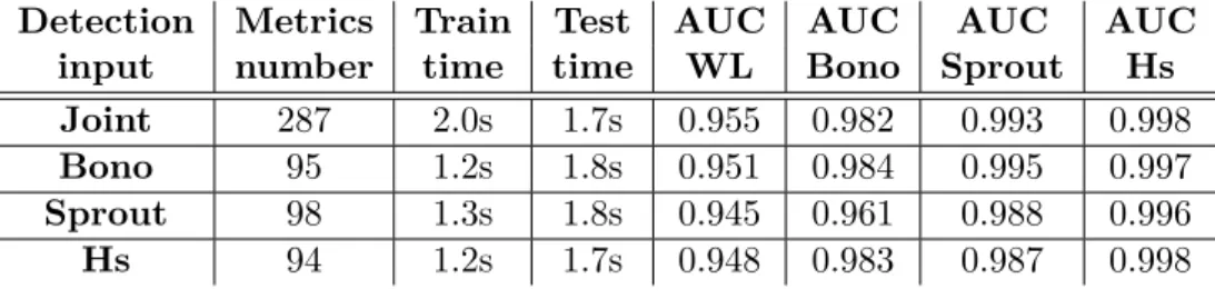
6.2.2 Per-VM detection: comparison of results

In this section we present the results of detection with data from a single VM in the case of black-box data. The aim is to compare the results obtained with those achieved with the joint approach, and record the computation times. As before, this section should allow us to decide whether having more data is the best choice, considering the increase in predictive ability and/or computation time. AUC and computation times are shown for 64 trees in table 10.

Table 10: Predictions of SLAV: all metrics versus single VM, detection with root cause localisation, black-box.

Detection Metrics Train Test AUC AUC AUC AUC

input number time time WL Bono Sprout Hs

Joint 287 2.0s 1.7s 0.955 0.982 0.993 0.998

Bono 95 1.2s 1.8s 0.951 0.984 0.995 0.997

Sprout 98 1.3s 1.8s 0.945 0.961 0.988 0.996

Hs 94 1.2s 1.7s 0.948 0.983 0.987 0.998

These results show that, as it happened in the case grey-box monitoring, predictive ability is improved for all SLAVs with the joint approach. However computation time also increases with more variables. Training time only increases slightly and testing time does not increase. These results show that, with black-box monitoring data, the joint approach provides the best results as while using grey-box monitoring.

6.2.3 Principal Component Analysis with Joint Approach

As in the grey-box case, PCA is performed on the variables used in the joint approach, and several numbers of components are used to test the results of the random forest algorithm which are shown in table 11 for 10, 17 and 110 components. The choice of this number of components is done for three typical specific PCA criteria. The choice of 10 components would

(27)

be justified by ease of interpretation, that of 17 by keeping the components with a variance higher than 1, and that of 110 components by the cumulative variance, which is 91% at this point and can therefore allow us to compare it to the 100 case for the PCA on grey-box metrics.

Table 11: AUC for PCA with 50 trees, black-box Detection

PCA 12 AUC 0.975 0.940 0.983 0.934

PCA 17 AUC 0.970 0.973 0.988 0.940

PCA 110 AUC 0.986 0.957 0.992 0.955

As it was expected from previous results, we can see that predictive ability improves with a higher number of dimensions, although the improvement is not great from 17 components to 110, as AUC increases on average by only 0.005. In addition, results measured by AUC are worse for the components providing 91% variance of black-box metrics than those with the same cu-mulative variance of grey-box metrics. All these results are therefore in line with previous conclusions.

6.3 Results with data from both monitoring sources

It has been shown by previous results that, in general, detections com-puted using metrics from black-box monitoring obtain lower results for each one of the selection approaches than those obtained from grey-box moni-toring. In this section we try to ascertain the cause of this difference. Two potential causes have been identified: firstly, the larger number of metrics in grey-box, and secondly the higher frequency of the recordings. In fact, the number of recordings in grey-box monitoring is approximately double that of black-box monitoring. To be able to compare these two datasets on a variable basis only, it is necessary to reduce the datasets to a common num-ber of observations recorded at the same times. In our data it was possible to do that and maintain 6568 common observations. This section will shed light on the relative importance of the amount of variables and the amount of observations in predictive ability.

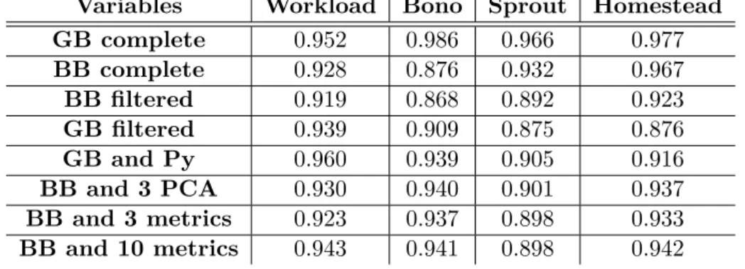
We have chosen 1064 trees in this case to ensure we have the most accu-rate results before comparing the performances of these metrics for SLAV detection. Results in terms of Precision-Recall AUC are presented in ta-ble 12. We call filtered the dataset with the common observations between grey-box and black-box. Results show that the number of observations plays

(28)

an important role in the accuracy of the random forest algorithm. In fact, the results obtained with grey-box and black-box data in this case are ap-proximately the same. Nevertheless, several important metrics have been identified, that would improve detection accuracy with black-box metrics if they were to be included. These results are shown as BB and 3 metrics, which correspond to the most highly-correlated variables of the three princi-pal components with the highest variance in PCA on grey-box metrics. We also include detection results with these 3 principal components added to black-box metrics, presented as BB and 3 PCA. We can see that, in either case, adding only these three variables to the black-box dataset is enough to improve results, which are close to those obtained will all grey-box and black-box metrics combined.

Table 12: Predictions of SLAV with different variables: all vms, 1064 trees, detection with root cause localisation, grey-box and black-box.

Variables Workload Bono Sprout Homestead

GB complete 0.952 0.986 0.966 0.977 BB complete 0.928 0.876 0.932 0.967 BB filtered 0.919 0.868 0.892 0.923 GB filtered 0.939 0.909 0.875 0.876 GB and Py 0.960 0.939 0.905 0.916 BB and 3 PCA 0.930 0.940 0.901 0.937 BB and 3 metrics 0.923 0.937 0.898 0.933 BB and 10 metrics 0.943 0.941 0.898 0.942

7 Detection results of errors

7.1 Results with data from grey-box monitoring

Results of error detection with data from grey-box monitoring are not pre-sented in this document. The reason for this is that no useful conclusion can be drawn from these results. These results are similar to those obtained with black-box monitoring, and better than those obtained with SLA violation detection. However, our preeminent aim in this study is to assess detec-tion results with black-box monitoring data, as we present in the following section.

(29)

7.2 Results with data from black-box monitoring

In this section we present detection results for errors. The results are shown in table 13 for error detection with random forest (64 trees) and black-box metrics. Results for error detection are very good compared to SLA violations for the black-box case, with the ROC AUC average being of 0.996 for error detection and only of 0.991 in the case of SLA violation detection.

Table 13: AUC for error detection: all metrics with 64 trees, black-box Number

Measure Cause in Cause in Cause in

of trees Bono Sprout Homestead

64 AUC 0.990 0.997 1.000

7.3 Results of detection with component localisation

In this section the aim is to detect all errors, in which machine they occur as well as in which component. In this case we no longer have 4 fault types but 15 (there are 3 VMs and 5 fault types for each of them). In this case, results are best with many trees, so they are shown for 1064 trees, as in general a larger number of classes requires a larger number of trees to produce equally accurate results.

In table 14, results are shown for error detection with grey-box as well as black-box data. The results show that all types of faults are detected with reasonable predictive ability. However, in the case of black-box monitoring, the same method produces bad results for errors 5,12 and 13. A possible explanation for these results is that the lower frequency of the recordings with black-box monitoring in this case might be critical when detecting these rare errors.

8 Sensitivity analysis of the Random Forest

algo-rithm

This section constitutes a discussion on the best ways to proceed in order to obtain good results in fault detection with random forest. Based on the results presented previously, this section addresses two choices that have to be made: the maximum number of decision nodes for the trees in random

(30)

Table 14: ROC AUC for errors detection with component localisation: all metrics with 1064 trees

Fault code Grey-box monitoring Black-box monitoring

1 0.966 0.955 2 0.999 1.000 3 1.000 1.000 5 1.000 0.998 6 1.000 1.000 12 1.000 0.970 13 1.000 0.592 15 0.997 1.000 16 0.999 1.000 17 1.000 1.000 22 0.999 0.994 23 1.000 1.000 25 1.000 1.000 26 1.000 0.999 27 1.000 1.000

forest and the number of trees. In the previous sections results were pre-sented with no maximum number of nodes and 64 trees, and this section will clarify the reasons for such choice.

8.1 Maximum number of nodes

An interesting parameter in random forest algorithm is the maximum number of nodes in a decision tree, i.e. the maximum depth of the tree. In results presented in previous sections we chose not to establish a maximum number of nodes, so that the algorithm can select any number. In this section we present the results obtained while varying this parameter. In particular, we use the example of detection of SLA violations with a joint approach based on grey-box monitoring. Results are shown in table 15 for different numbers of nodes, in terms of predictive ability of the models obtained as well as training and testing times.

As we can see in these results, predictive ability improves notably when the number of decision nodes increases, which was the result we expected. In addition, we observe that there is no increase in testing time (the supplemen-tary decisions which have to be made seem to have a negligible computation time) and the increase in training time is not very large. For example, only 0.6 seconds separate the execution times with 3 maximum nodes and with no

(31)

Table 15: Predictions of SLAV with different number of nodes: all vms, 50 trees, detection with root cause localisation, grey-box.

Maximum 3 5 7 10 15 No maximum Train time 3.7s 3.6s 3.7s 3.9s 4.0s 4.3s Test time 1.8s 1.8s 1.8s 1.9s 1.8s 1.8s Workload PR 0.862 0.912 0.930 0.943 0.958 0.978 Bono PR 0.875 0.911 0.941 0.953 0.964 0.980 Sprout PR 0.798 0.884 0.917 0.945 0.965 0.978 Homestead PR 0.578 0.751 0.842 0.881 0.919 0.948

maximum number of nodes. Therefore we believe that imposing a maximum number of nodes is not advisable.

8.2 Number of trees

In this section we explain the results obtained with different numbers of trees in order to select the appropriate one for this dataset. The reason for this is that selecting the appropriate number of trees for the random forest algorithm prior to testing is not straightforward. In theory, results should get better on average as the number of trees increases. However, the improvement by adding trees is a decreasing function, and at some point the benefit of adding more trees is insignificant and not worth the computational cost. For example, in the tests performed on our small dataset, computation takes under five seconds with 32 trees, versus almost a minute for 1064 trees. Results do not seem to improve much beyond this number of trees, so it will be considered as a maximum in this case. The example used here to explain the choice of the number of trees is that of SLA detection with grey-box monitoring data and a joint approach. AUC are shown in table 16 for four tree number choices, namely 10, 32, 64 and 1064 trees.

Table 16: AUC for all metrics with different number of trees, grey-box Number

10 AUC 0.999 0.998 0.999 0.947

32 AUC 0.999 0.999 0.999 0.959

64 AUC 0.999 0.999 0.999 0.961

(32)

As we can see in table 16, results improve generally with the number of trees. However, the improvement decreasing with the number of trees, we can see that the difference between 64 and 1064 trees is probably not worth the computational cost. We will therefore establish 64 trees as a reasonable amount for this dataset. The results showing precision and recall for each fault type are shown in table 17.

Table 17: Predictions of SLAV: all metrics combined, detection with root cause localisation, grey-box.

Number

Precision 0.99 0.91 0.97 0.85 10 Recall 0.64 0.64 0.71 0.90 F1-score 0.78 0.75 0.82 0.88 Precision 0.98 0.96 1.00 0.85 32 Recall 0.59 0.65 0.60 0.94 F1-score 0.74 0.78 0.75 0.89 Precision 0.98 0.98 0.98 0.85 64 Recall 0.59 0.63 0.63 0.93 F1-score 0.74 0.77 0.77 0.89 Precision 0.98 0.98 0.98 0.86 1064 Recall 0.55 0.62 0.60 0.94 F1-score 0.71 0.76 0.74 0.90

As we can see, these results are discouraging compared to those expected. In fact, our problem relies on the choice of the appropriate alarm threshold. The result of random forest is a probability, and it has to be decided when to signal a fault or not. A 0 threshold yields 1.00 recall and low precision, while a threshold close to 1 would give high precision and low recall. These bad results in table 17 are due to a suboptimal choice of this threshold. In fact, a better threshold would greatly improve results, as shown in table 18 for the 64-tree case, where we have not changed the threshold for the high workload detection as it was already a sensible one.

In conclusion, we can establish 64 trees as a reasonable value for this parameter in Random Forest algorithm. For comparison purposes, we have

(33)

Table 18: Predictions of SLAV: all metrics combined, detection with root cause localisation, grey-box.

Number

Precision 0.94 0.94 0.94 0.85

64 Recall 0.94 0.93 0.90 0.93

F1-score 0.94 0.93 0.92 0.89

maintained this number in all our tests with SLA detection. A similar method (not presented here) to the one described above allowed us to choose different numbers of trees for all the other tests carried out in this study. In particular, we have found 1064 trees to be a reasonable value for detection with component localisation and 50 trees for tests with PCA. The reason for this is that a data set with fewer variables requires less trees, whereas detection with more classes requires more trees.

9 Other methods

9.1 Detection with time series

Having analysed the results obtained with the random forest algorithm, a different approach to the problem has been tested, using a method that does not require training a model prior to SLAV detection. The method used is Bayesian Change Point (BCP) detection in time series, implemented using the BCP R package [4]. It comes from time series analysis which takes into account the order of the observations in the data, which are collected in regular fifteen-second intervals.

BCP is tested for detection using the original variables described previ-ously, as well as the PCA components. The SLAV detection is performed for the binary case with only two classes, namely "SLA violation" or "no violation". The results for PCA components are shown in table 19.

Table 19: Predictions of SLAV with BCP: PCA components, binary detec-tion, grey-box.

Results PCA PCA PCA PCA PCA

2 3 4 5 10

(34)

We can see from the results shown in table 20 that predictive ability with the BCP method actually decreases with the number of variables. In order to confirm this intuition, we tried BCP on the complete dataset with 360 variables, for binary detection. Results obtained an AUC of 0.42, which confirms the idea that BCP does not achieve good predictions with many variables. Several other tests were performed with a few grey-box metrics, as we enumerate below:

• The first (most correlated) variable describing each of the first five principal components

• The first 10 variables of the first principal component – Detection of SLA violation against no violation

– Detection of network-related violations against no violation (NW) – Detection of network-related violations and high workload (NW

& WL)

– Detection of high workload only (WL)

Results for BCP on the original variables are shown in table 20.

Table 20: Predictions of SLAV with BCP: original variables, binary detec-tion, grey-box.

Results First five First ten First ten First ten First ten

variables SLA NW WL NW & WL

AUC 0.65 0.72 0.55 0.72 0.71

These results show that predictions are not very reliable with this method. The time series approach with black-box data is expected to yield similar results to those obtained in the case of grey-box data. The only test made with all variables results in a ROC AUC of 0.43, very close to that obtained with grey-box metrics.

9.2 Detection with gaussian mixture models

In this section we present a second alternative approach to random forest that we have investigated. This method is called Gaussian Mixture

Mod-els (GMM) and we tested it using its python implementation [9]. This

method consists in separating the observations into groups according to a number of gaussian distributions chosen in advance. To do this it relies on

(35)

the Expectation-Maximisation Algorithm to calculate the means and covari-ance matrices of these distributions by maximising the probability of these realisations under the assumption that they follow one of the gaussian dis-tributions. This can be seen as a generalisation of the k-means clustering algorithm. The main problem we encountered is that, when using many clusters, it is difficult to provide a decision rule to decide which clusters cor-respond to anomalies. We therefore tried binary detection, yet results were unsatisfactory and we cannot draw any conclusions from them. Therefore these results are not presented in this document.

On the contrary, this method has a supervised approach which did produce good results. The difference is that with this approach the means of the gaussian distributions for each class are given in advance, according to the data available. This method achieves much better results, however it is out of the scope of our section, which aim was to provide a viable unsupervised alternative to Random Forest. This is why these results are not presented in this document either.

10 Conclusion

In this document we analyse several detection problems in a particular case study by means of the Random Forest algorithm and other unsuper-vised learning methods, focusing in particular in detection with VM granu-larity and black-box data. This study shows most clearly that, in our case, performing a PCA on monitoring data reduces predictive ability when using Random Forest algorithm. This result was observed in all cases, regardless of the virtual machine or monitoring source considered, as well as the pa-rameters of the algorithm. These results suggest that the performance of Random Forest algorithm is not affected by information redundancy or a large number of dimensions.

In addition, this case study shows that results are better with grey-box than black-box monitoring. Nevertheless, the reason for this difference in this case is more related to the higher frequency of the observations than the quality of the predictors obtained with the monitoring sources. This result highlights the importance of having a large amount of observations and sug-gests that anomaly detection with black-box or grey-box monitoring might achieve equally good results in similar conditions. Finally, this study shows that in our case, the unsupervised learning methods tested were ineffective for anomaly detection for different reasons.

(36)

References

[1] E. Aleskerov, B. Freisleben, and B. Rao. Cardwatch: a neural net-work based database mining system for credit card fraud detection. In

Computational Intelligence for Financial Engineering (CIFEr), 1997., Proceedings of the IEEE/IAFE 1997, pages 220–226, Mar 1997.

[2] A. Avizienis, J.-C. Laprie, B. Randell, and C. Landwehr. Basic concepts and taxonomy of dependable and secure computing. Dependable and

Secure Computing, IEEE Transactions on, 1(1):11–33, 2004.

[3] D.E. Denning. An intrusion-detection model. Software Engineering,

IEEE Transactions on, SE-13(2):222–232, Feb 1987.

[4] Chandra Erdman, John W Emerson, et al. bcp: an r package for performing a bayesian analysis of change point problems. Journal of

Statistical Software, 23(3):1–13, 2007.

[5] L. Heberlein. Network security monitor (nsm)–final report. 1995. [6] Wenke Lee, S.J. Stolfo, and K.W. Mok. A data mining framework for

building intrusion detection models. In Security and Privacy, 1999.

Proceedings of the 1999 IEEE Symposium on, pages 120–132, 1999.

[7] Wenke Lee and Dong Xiang. Information-theoretic measures for anomaly detection. In Security and Privacy, 2001. S P 2001.

Pro-ceedings. 2001 IEEE Symposium on, pages 130–143, 2001.

[8] D. Michie, D. J. Spiegelhalter, and C.C. Taylor. Machine learning, neural and statistical classification, 1994.

[9] F. Pedregosa, G. Varoquaux, A. Gramfort, V. Michel, B. Thirion, O. Grisel, M. Blondel, P. Prettenhofer, R. Weiss, V. Dubourg, J. Van-derplas, A. Passos, D. Cournapeau, M. Brucher, M. Perrot, and E. Duchesnay. Scikit-learn: Machine learning in Python. Journal of

Machine Learning Research, 12:2825–2830, 2011.

[10] Carla Sauvanaud, Kahina Lazri, Mohamed Kaâniche, and Karama Ka-noun. Anomaly detection and root cause localization in virtual net-work functions. In International Symposium on Software Reliability

Engineering, Ottawa, Canada.

[11] Carla Sauvanaud, Guthemberg Silvestre, Mohamed Kaâniche, and Karama Kanoun. Data Stream Clustering for Online Anomaly Detec-tion in Cloud ApplicaDetec-tions. In 11th European Dependable Computing

(37)

[12] Jiong Zhang, M. Zulkernine, and A. Haque. Random-forests-based net-work intrusion detection systems. Systems, Man, and Cybernetics, Part

C: Applications and Reviews, IEEE Transactions on, 38(5):649–659,

(38)