Supporting information

Serra, E., Valla, P. G., Gribenski, N., Guedes Magrani, F., Carcaillet, J., Delaloye, R., Grobety, B. & Braillard, L.:

Geomorphic response to the Lateglacial–Holocene transition in high Alpine regions (Sanetsch Pass, Swiss Alps).

2020. Boreas

https://doi.org/10.1111/bor.12480

. ISSN 0300-9483

Supporting information

Table S1. Samples locations, corresponding geomorphic units and conducted analyses.

Sample Name

Location WGS84

(°N/°E)

Altitude

(m a.s.l.)

Geomorphic unit

Analysis

G1 - G6

46.34091/ 7.29049

2100

Alluvial fan (CRE)

Grain-size

G7, G8

46.33703/ 7.31810

2712

High-elevation platform (ARP)

Grain-size

M1 - M3

46.34091/ 7.29049

2100

Alluvial fan (CRE)

Micromorphology

L1, L2; S1, S2

46.33715/ 7.31815;

46.33380/ 7.30790

2712;

2650

Bedrock

(limestone; shale)

Petrographic thin section

CRE01 - CRE16 46.34091/ 7.29049

2100

Alluvial fan (CRE)

XRD and Geochemistry

ARP01, ARP03 46.33703/ 7.31810

2712

High-elevation platform (ARP)

XRD and Geochemistry

L1, L2; S1, S2

46.33715/ 7.31815;

46.33380/ 7.30790

2712;

2650

Bedrock

(limestone; shale)

XRD

cre01 - cre16

46.34091/ 7.29049

2100

Alluvial fan (CRE)

Portable OSL

arp01 - arp05

46.33703/ 7.31810

2712

High-elevation platform (ARP)

Portable OSL

CRE01 - CRE04 46.34091/ 7.29049

2100

Alluvial fan (CRE)

OSL burial dating

ARP01 - ARP03 46.33703/ 7.31810

2712

High-elevation platform (ARP)

OSL burial dating

SAN01

46.35111/ 7.28751

2055

Rockfall deposit (SAN)

_{Be exposure dating}

SAN02

46.35117/ 7.28900

2056

Rockfall deposit (SAN)

_{Be exposure dating}

SAN03

46.35137/ 7.28874

2054

Rockfall deposit (SAN)

_{Be exposure dating}

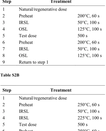
Table S2. Luminescence protocols. A. Post-IR OSL protocol, after Murray & Wintle (2000),

applied on quartz separates from CRE and ARP sample (except for sample ARP03, which did not

provide enough material for quartz purification

B. Post-IR IRSL protocol, after Buylaert et al.

(2009), applied on polymineral ARP samples. No post-IR IRSL measurements were performed on

CRE samples due to the absence of feldspar IRSL signal.

Table S2A

Step

Treatment

1

Natural/regenerative dose

2

Preheat

250°C, 60 s

3

IRSL

50°C, 100 s

4

IRSL

225°C, 100 s

5

Test dose

500 s

6

Preheat

250°C, 60 s

7

IRSL

50°C, 100 s

8

IRSL

225°C, 100 s

9

IRSL

290°C, 40 s

10

Return to step 1

Step

Treatment

1

Natural/regenerative dose

2

Preheat

200°C, 60 s

3

IRSL

50°C, 100 s

4

OSL

125°C, 100 s

5

Test dose

500 s

6

Preheat

200°C, 60 s

7

IRSL

50°C, 100 s

8

OSL

125°C, 100 s

9

Return to step 1

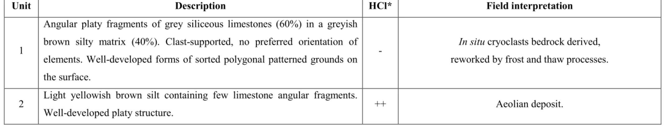
Table S3. Stratigraphic description and field interpretation of the sedimentological units forming the ARP high-elevation platform

deposit. The thickness of the units is given in Fig. 4. *Reaction to HCl on the field: no (-), little (-/+), strong (+), very strong (++)

reaction.

Unit Description HCl* Field interpretation

1

Angular platy fragments of grey siliceous limestones (60%) in a greyish brown silty matrix (40%). Clast-supported, no preferred orientation of elements. Well-developed forms of sorted polygonal patterned grounds on the surface.

- In situ cryoclasts bedrock derived,

reworked by frost and thaw processes. 2 Light yellowish brown silt containing few limestone angular fragments.

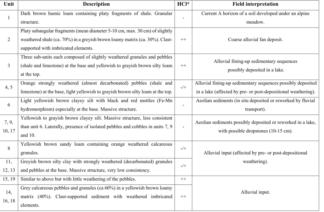
Table S4. Stratigraphic description and field interpretation of the sedimentological units forming the upper 4.5 m of the CRE alluvial

fan. The thickness of the units is given in Fig. 5. *Reaction to HCl on the field: no (-), little (-/+), strong (+), very strong (++) reaction.

Unit

Description

HCl*

Field interpretation

1 Dark brown humic loam containing platy fragments of shale. Granular

structure. -

Current A horizon of a soil developed under an alpine meadow.

2

Platy subangular fragments (mean diameter 5-10 cm, max. 30 cm) of slightly weathered shale (ca. 70%) in a greyish brown loamy matrix (ca. 30%). Clast-supported with imbricated elements.

++ Coarse alluvial fan deposit.

3

Three sub-units each composed of slightly weathered granules and pebbles (shale and limestone) at the base and yellowish to grayish brown silty loam at the top.

++ Alluvial fining-up sedimentary sequences possibly deposited in a lake. 4, 5 Orange strongly weathered (almost decarbonated) pebbles (shale and

limestone) at the base, light yellowish to grayish brown silty loam at the top. -/+

Alluvial fining-up sedimentary sequences possibly deposited in a lake (affected by pre- or post-depositional weathering). 6 Light yellowish brown clayey silt with black and red mottles (Fe-Mn

hydromorphism) especially at the base. Massive structure. -

Aeolian sediments (in situ deposited or reworked by fluvial transport).

7, 9, 10, 17

Yellowish to grayish brown clayey silt. Massive structure, less consistent than unit 6. Laterally, presence of isolated pebbles and cobbles in units 7, 9 and 10.

- Aeolian sediments possibly deposited or reworked in a lake, with possible dropstones (10-15 cm).

8 Yellowish brown sandy loam containing orange weathered calcareous

granules. -/+ Alluvial input (affected by pre- or post-depositional

weathering). 11,

12, 13

Greyish brown silty clay with strongly weathered (decarbonated) granules and pebbles at the base. Massive structure, very low consistency. -/+ 15, 19 Similar to above but with little weathering of the pebbles. ++

Alluvial input. 14,

16, 18

Grey calcareous pebbles and granules (ca 60%) in a yellowish brown loamy matrix (40%). Clast-supported sediment with weathered imbricated elements.

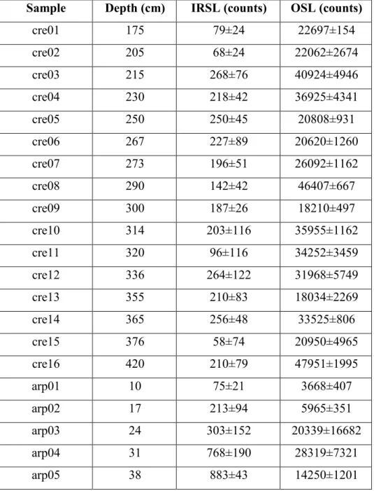
Table S5. Luminescence signal intensities measured for CRE and ARP sites using the

. IRSL counts are the total photon counts obtained after the first 30 s of IRSL

stimulation. OSL counts are the total photon counts obtained after the 60 s of OSL stimulation.

The counts and respective errors were obtained by averaging between two replicate

measurements of each bulk sediment sample.

Dim IRSL counts were measured along the CRE

section, due to the low-feldspar content in the analysed sediments. For this reason, only the

OSL signal intensity profile is represented in Fig. 10.

Sample

Depth (cm)

IRSL (counts)

OSL (counts)

cre01

175

79±24

22697±154

cre02

205

68±24

22062±2674

cre03

215

268±76

40924±4946

cre04

230

218±42

36925±4341

cre05

250

250±45

20808±931

cre06

267

227±89

20620±1260

cre07

273

196±51

26092±1162

cre08

290

142±42

46407±667

cre09

300

187±26

18210±497

cre10

314

203±116

35955±1162

cre11

320

96±116

34252±3459

cre12

336

264±122

31968±5749

cre13

355

210±83

18034±2269

cre14

365

256±48

33525±806

cre15

376

58±74

20950±4965

cre16

420

210±79

47951±1995

arp01

10

75±21

3668±407

arp02

17

213±94

5965±351

arp03

24

303±152

20339±16682

arp04

31

768±190

28319±7321

arp05

38

883±43

14250±1201

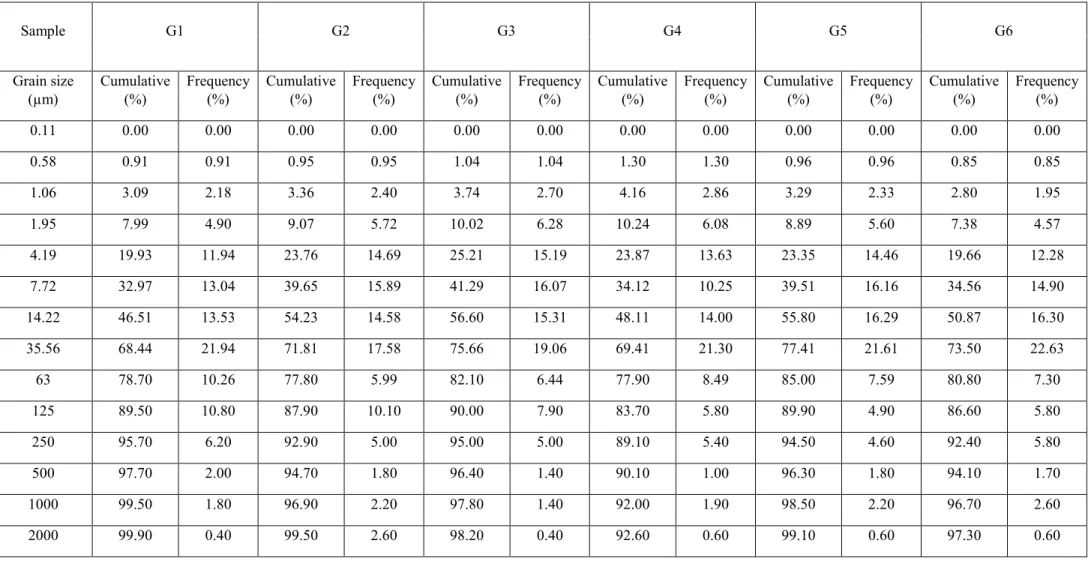
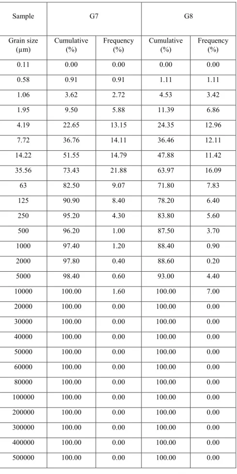
Table S6. Grain-size distributions of CRE (G1-G6; S6A) and ARP (G7 and G8; S6B) samples. Individual cumulative and frequency percentages of the different

grain sizes are reported. Details about

grain-size distribution measurements

Table S6A. Grain-size distributions of CRE samples.

Sample G1 G2 G3 G4 G5 G6

Grain size

(µm) Cumulative (%) Frequency (%) Cumulative (%) Frequency (%) Cumulative (%) Frequency (%) Cumulative (%) Frequency (%) Cumulative (%) Frequency (%) Cumulative (%) Frequency (%)

0.11 0.00 0.00 0.00 0.00 0.00 0.00 0.00 0.00 0.00 0.00 0.00 0.00 0.58 0.91 0.91 0.95 0.95 1.04 1.04 1.30 1.30 0.96 0.96 0.85 0.85 1.06 3.09 2.18 3.36 2.40 3.74 2.70 4.16 2.86 3.29 2.33 2.80 1.95 1.95 7.99 4.90 9.07 5.72 10.02 6.28 10.24 6.08 8.89 5.60 7.38 4.57 4.19 19.93 11.94 23.76 14.69 25.21 15.19 23.87 13.63 23.35 14.46 19.66 12.28 7.72 32.97 13.04 39.65 15.89 41.29 16.07 34.12 10.25 39.51 16.16 34.56 14.90 14.22 46.51 13.53 54.23 14.58 56.60 15.31 48.11 14.00 55.80 16.29 50.87 16.30 35.56 68.44 21.94 71.81 17.58 75.66 19.06 69.41 21.30 77.41 21.61 73.50 22.63 63 78.70 10.26 77.80 5.99 82.10 6.44 77.90 8.49 85.00 7.59 80.80 7.30 125 89.50 10.80 87.90 10.10 90.00 7.90 83.70 5.80 89.90 4.90 86.60 5.80 250 95.70 6.20 92.90 5.00 95.00 5.00 89.10 5.40 94.50 4.60 92.40 5.80 500 97.70 2.00 94.70 1.80 96.40 1.40 90.10 1.00 96.30 1.80 94.10 1.70 1000 99.50 1.80 96.90 2.20 97.80 1.40 92.00 1.90 98.50 2.20 96.70 2.60 2000 99.90 0.40 99.50 2.60 98.20 0.40 92.60 0.60 99.10 0.60 97.30 0.60

5000 100.00 0.10 99.60 0.10 99.10 0.90 96.30 3.70 99.80 0.70 98.50 1.20 10000 100.00 0.00 100.00 0.40 100.00 0.90 100.00 3.70 100.00 0.20 100.00 1.50 20000 100.00 0.00 100.00 0.00 100.00 0.00 100.00 0.00 100.00 0.00 100.00 0.00 30000 100.00 0.00 100.00 0.00 100.00 0.00 100.00 0.00 100.00 0.00 100.00 0.00 40000 100.00 0.00 100.00 0.00 100.00 0.00 100.00 0.00 100.00 0.00 100.00 0.00 50000 100.00 0.00 100.00 0.00 100.00 0.00 100.00 0.00 100.00 0.00 100.00 0.00 60000 100.00 0.00 100.00 0.00 100.00 0.00 100.00 0.00 100.00 0.00 100.00 0.00 80000 100.00 0.00 100.00 0.00 100.00 0.00 100.00 0.00 100.00 0.00 100.00 0.00 100000 100.00 0.00 100.00 0.00 100.00 0.00 100.00 0.00 100.00 0.00 100.00 0.00 200000 100.00 0.00 100.00 0.00 100.00 0.00 100.00 0.00 100.00 0.00 100.00 0.00 300000 100.00 0.00 100.00 0.00 100.00 0.00 100.00 0.00 100.00 0.00 100.00 0.00 400000 100.00 0.00 100.00 0.00 100.00 0.00 100.00 0.00 100.00 0.00 100.00 0.00 500000 100.00 0.00 100.00 0.00 100.00 0.00 100.00 0.00 100.00 0.00 100.00 0.00

Table S6B. Grain-size distributions of ARP samples.

Sample G7 G8

Grain size

(µm) Cumulative (%) Frequency (%) Cumulative (%) Frequency (%)

0.11 0.00 0.00 0.00 0.00 0.58 0.91 0.91 1.11 1.11 1.06 3.62 2.72 4.53 3.42 1.95 9.50 5.88 11.39 6.86 4.19 22.65 13.15 24.35 12.96 7.72 36.76 14.11 36.46 12.11 14.22 51.55 14.79 47.88 11.42 35.56 73.43 21.88 63.97 16.09 63 82.50 9.07 71.80 7.83 125 90.90 8.40 78.20 6.40 250 95.20 4.30 83.80 5.60 500 96.20 1.00 87.50 3.70 1000 97.40 1.20 88.40 0.90 2000 97.80 0.40 88.60 0.20 5000 98.40 0.60 93.00 4.40 10000 100.00 1.60 100.00 7.00 20000 100.00 0.00 100.00 0.00 30000 100.00 0.00 100.00 0.00 40000 100.00 0.00 100.00 0.00 50000 100.00 0.00 100.00 0.00 60000 100.00 0.00 100.00 0.00 80000 100.00 0.00 100.00 0.00 100000 100.00 0.00 100.00 0.00 200000 100.00 0.00 100.00 0.00 300000 100.00 0.00 100.00 0.00 400000 100.00 0.00 100.00 0.00 500000 100.00 0.00 100.00 0.00

Table S7. XRD bulk mineralogical compositions of CRE (CRE01-CRE16), ARP (ARP01 andARP03) and

bedrock (L1-L2: siliceous limestone, S1-S2: calcareous shale) samples. Cumulative mineral percentages are reported. Details about

XRD analyses

Sample Quartz (%) Micas (%) Chlorite (%) Albite (%) Calcite (%) Dolomite (%)

CRE01 36.9 42.5 10.6 0.0 10.0 0.0 CRE02 39.2 51.5 9.3 0.0 0.0 0.0 CRE03 50.0 36.0 14.0 0.0 0.0 0.0 CRE04 42.7 22.5 9.9 11.1 13.9 0.0 CRE05 54.4 41.8 3.8 0.0 0.0 0.0 CRE06 46.5 41.3 12.2 0.0 0.0 0.0 CRE07 46.7 40.5 12.8 0.0 0.0 0.0 CRE08 51.4 40.6 8.0 0.0 0.0 0.0 CRE09 41.1 50.8 8.1 0.0 0.0 0.0 CRE10 52.9 39.5 7.6 0.0 0.0 0.0 CRE11 54.0 44.9 1.1 0.0 0.0 0.0 CRE12 43.3 36.1 8.4 0.0 12.3 0.0 CRE13 41.6 38.2 7.9 0.0 12.3 0.0 CRE14 32.4 22.9 6.3 0.0 38.5 0.0 CRE15 41.8 42.9 9.8 0.0 5.5 0.0 CRE16 35.6 30.3 7.4 0.0 26.6 0.0 ARP01 69.6 18.9 7.6 3.9 0.0 0.0 ARP03 66.7 18.2 8.0 7.1 0.0 0.0 L1 25.6 5.6 0.0 0.0 63.7 5.2 L2 32.7 3.0 0.0 0.0 64.3 0.0 S1 23.7 15.5 0.8 0.0 55.1 4.9 S2 22.5 7.0 4.0 0.0 65.9 0.9