Tomography of subduction zones using regional earthquakes: methodological developments and application to the Ionian slab.

(1)

HAL Id: tel-00438598

https://tel.archives-ouvertes.fr/tel-00438598

Submitted on 16 Jan 2013

HAL is a multi-disciplinary open access archive for the deposit and dissemination of sci-entific research documents, whether they are pub-lished or not. The documents may come from teaching and research institutions in France or abroad, or from public or private research centers.

L’archive ouverte pluridisciplinaire HAL, est destinée au dépôt et à la diffusion de documents scientifiques de niveau recherche, publiés ou non, émanant des établissements d’enseignement et de recherche français ou étrangers, des laboratoires publics ou privés.

Tomography of subduction zones using regional

earthquakes: methodological developments and

application to the Ionian slab.

Marco Calo’

To cite this version:

Marco Calo’. Tomography of subduction zones using regional earthquakes: methodological develop-ments and application to the Ionian slab.. Geophysics [physics.geo-ph]. Université de Strasbourg, 2009. English. �tel-00438598�

(2)

Thèse en cotutelle

présentée pour obtenir le grade de Docteur de

l’Université de Strasbourg et de l’Université de Messine

par

Marco Calò

Tomography of subduction zones using regional

earthquakes: methodological developments and

application to the Ionian slab.

Tomographie des zones en subduction en utilisant les

séismes locaux: développements méthodologiques et

applications pratiques à la plaque Ionienne.

Soutenue publiquement le 19 mars 2009

Discipline : Géophysique / Geofisica per l’Ambiente e il Territorio XXI ciclo

Directeur de Thèse : Dr. Catherine Dorbath E.O.S.T. Strasbourg

Co-directeur de Thèse : Pr. Dario Luzio C.F.T.A. Palermo

Rapporteur Interne : Pr. Frédéric Masson I.P.G. Strasbourg

Rapporteur Externe : Dr. Serge Lallemand C.N.R.S. Montpellier

Rapporteur Externe : Pr. Attilio Sulli Dip. di Geologia Palermo

Examinateur : Pr. Domenico Schiavone Dip. di Geologia Bari

(3)

(4)

To my love,

and to my grandparents.

(5)

(6)

Résumé

Dans les modèles géodynamiques les plus couramment admis, la sismicité intermédiaire et profonde de la zone Tyrrhénienne méridionale et de l'arc de la Calabre a été attribuée à un processus assez développé de subduction de la lithosphère océanique, où la lithosphère Ionienne s'enfonce sous la lithosphère de la mer Tyrrhénienne amincie, jusqu'à environ 500 km de profondeur. L'archipel des îles Éoliennes et les monts sous-marins voisins sont aussi associés au processus de subduction, et la Mer Tyrrhénienne méridionale interprétée comme bassin arrière-arc.

L'hétérogénéité des mécanismes des sources sismiques présentes dans la Mer Tyrrhénienne méridionale, en Sicile et en Calabre témoigne de la complexité du processus géodynamique en cours. L'étude de cette zone présente encore de nombreuses questions ouvertes, dues aux connaissances limitées des unités géologiques sur lesquels agissent les forces, et en particulier au détail insuffisant des modèles géophysiques de la lithosphère.

Les techniques tomographiques utilisées jusqu’aujourd'hui dans la région tyrrhénienne ont contribué à déterminer à grande échelle les structures géologiques de la croûte et du manteau supérieur, mais elles n'ont pas une résolution suffisante pour distinguer les différentes unités qui les constituent.

De plus, souvent, les analyses de la fiabilité des estimations de vitesse et de la stabilité du problème inverse traité, qui sont des paramètres fondamentaux pour une étude géophysique, sont peu développées.

La reconstruction détaillée de la géométrie actuelle de la subduction Ionienne et des structures de la lithosphère de la Mer Tyrrhénienne méridionale et de l'Italie sud-occidentale pourrait fournir d’importants apports pour la définition d'un modèle cinématique évolutif de la mer Tyrrhénienne entière. En outre, la détermination et la description détaillée des structures responsables de l'activité sismique présente dans le secteur Calabro-Sicilien et les bassins environnants pourraient apporter des contributions considérables à la modélisation de la sismicité dans les domaines de l’espace, du temps et de la magnitude.

L'étude détaillé des structures lithosphériques et intramantelliques présentes dans cette partie de l'Italie méridionale a été réalisée, pendant cette thèse de doctorat, en effectuant une tomographie sismique tridimensionnelle à résolution élevée en ondes de volume.

Les principaux développements de cette thèse peuvent être résumés en trois principales sections: dans la première, qui comprend les chapitres 1 et 2, on retrace synthétiquement l’histoire de the la tomographie sismique et les méthodes proposées pendant les vingt dernier années. Le deuxième chapitre est entièrement dédié à l’explication du programme d’inversion TomoDD (Zangh and Thurber, 2003), choisi pour réaliser les premiers images tomographiques, qui utilise la méthode de la double-différence pour l'obtention de la solution du problème inverse tomographique.

Dans la deuxième partie (chapitres 3 et 4), on développe les aspects méthodologiques et théoriques pour la réalisation d’une tomographie à haute résolution en mettant en oeuvre une nouvelle technique de post-processing appelée WAM (Weighted Average Model).

Comme données expérimentales, on a utilisé les enregistrements des tremblements de terre s’étant produits en Italie méridionale depuis 1981 jusqu'en 2005, effectués par les stations du réseau sismique national italien et des réseaux locaux. Seuls les séismes enregistrés par plus de 10 stations, et localisés avec un RMS (Root Mean Square) inférieur à 0.5 s avec un modèle 1D optimal de la région d’étude, ont été sélectionnés pour la réalisation de la tomographie.

(7)

Cette partie du travail de thèse a visé à la réalisation des nombreux tests avec des données synthétiques et des données expérimentales, pour évaluer la dépendance du modèle final d’une tomographie « DD classique » aux paramètres initiaux.

En particulier, on a appliqué le « resolution restoration test » (Zhao et al., 1992) comme test synthétique pour évaluer la capacité des données sélectionnées à reconstruire la distribution du champ de vitesse obtenu par une inversion expérimentale. La dépendance du modèle final aux conditions initiales a été évaluée en réalisant trois types de tests expérimentaux : 1) estimation de la dépendance du modèle de vitesse final à la grille d’inversion utilisée en faisant plusieurs inversions en changeant la géométrie de la grille; 2) estimation de la dépendance du modèle final au modèle initial en faisant des inversions tomographiques avec différents modèles initiaux 1D et 3D ; 3) estimation de la dépendance du modèle final à la sélection des données expérimentales et au système de pondération entre les donnés absolues et relatives en faisant de multiples inversions en changeant les règles de sélection des données et le système de pondération.

Tous les tests ont démontré qu' une inversion tomographique réalisée en utilisant les données et la méthode choisie produisent des modèles 3D de vitesse Vp et Vs très détaillés et fiables pour la description de la géométrie des corps présents jusqu’à la profondeur de 350 km. Par contre, l’estimation des valeurs absolues de vitesse dans certaines parties des modèles a montré une variabilité et une dépendance aux conditions initiales qui ne permettaient pas d'utiliser les résultats pour en faire une interprétation pétrologique. Pour surmonter ces limitations, on a imaginé de réaliser un modèle moyen pratiquement indépendant des conditions initiales et donc plus fiable. La construction du modèle moyen est réalisée en faisant un re-échantillonnage des nombreux modèles de vitesse, déjà produits avec tomoDD, dans un grille fixée (WAM grid), en utilisant la même règle d’interpolation que celle utilisée par le programme de tomographie. Dans notre cas la règle d’interpolation est tri-linéaire. Les valeurs de DWS (Derivative Weight Sum, Toomey and

Foulger, 1989), paramètre lié à la quantité d’information expérimentale utilisée pour

estimer la valeur de la vitesse à chaque nœud du modèle, sont aussi interpolées dans un grille identique. La valeur de DWS a été utilisée comme facteur de pondération dans le calcul de la vitesse moyenne, ainsi dans les nœuds de la WAM grid on pourra donner plus de poids à une valeur de vitesse estimée avec plus de résolution pendant les inversions tomographiques.

Les valeurs de la déviation standard et la DWS du modèle WAM sont calculées avec la même méthode.

Pour évaluer l'efficacité de la méthode de pondération et la validité du modèle de vitesse WAM, on a réalisé un test synthétique de type échiquier intégré avec l’estimation d’un paramètre de restauration (R) qui donne une estimation quantitative (exprimée en %) de la capacité de reconstruction du modèle. De plus, en comparant la distribution de R et la déviation standard, on a pu vérifier qu'il existe une loi d' anti-corrélation entre ces deux paramètres: dans les parties du modèle synthétique WAM où l'on trouve des hautes valeurs de déviation standard on trouve des faibles valeurs de R et vice versa. Par ce moyen, on a pu lier directement le paramètre quantitatif du pouvoir de restauration (R) à la déviation standard du modèle expérimental WAM.

En principe, la méthode WAM, étant un post-processing, pourrait être utilisée avec chaque programme de tomographie, permettant ainsi d'obtenir une plus grande fiabilité des modèles pour leur interprétation.

Dans la troisième partie de la thèse (chapitres 5 et 6), on a appliqué la méthode WAM à l'Italie du Sud. La grande fiabilité du modèle WAM obtenu avec une haute résolution a nous permis la reconstruction de la géométrie des corps intérieurs au slab Ionien et au manteau tyrrhénien. La première caractéristique des modèles WAM pour les vitesses des ondes P et S est la présence de corps à faible vitesse (7.0 < Vp < 7.7 km/s et 3.8 < Vs < 4.2

(8)

km/s) jusqu’à la profondeur de 220-250 km dans le slab en subduction par ailleurs caractérisé par des valeurs hautes (8.2 < Vp < 8.8 km/s et 4.75 < Vs < 5 km/s).

Ces corps ont des dimensions variables, entre 15 et 35 km de largeur et 35 à 55 km de longueur, et sont compatibles avec zones de la lithosphère ionienne serpentinisées à 20-30 % (Christensen, 2004).

L’hydratation de l’ harzburgite à serpentine est provoquée par une partie des fluides du slab qui migrent dans la lithosphère par des zones plus poreuses comme les « fault bends ».

L’inclinaison du slab joue un rôle dominant pour la répartition des fluides qui migrent soit dans la lithosphère même soit dans le manteau autour (Abers, 2005).

A des profondeurs plus grandes, les conditions de température et pression font que le processus de déshydratation transforme les minéraux de la serpentine en phases de plus haute pression comme la phase « A » qui a des caractéristiques très similaires à l’ harzburgite anhydre (Fumagalli and Poli, 2005; Hacker et al., 2003).

Avec le WAM on a pu reconstruire la forme 3D du slab Ionienne et mettre en évidence sa géométrie très particulière qui peut être comparée à un sablier incliné de 69°-72° vers le N-W.

Dans le manteau Tyrrhénien, jusqu’à la profondeur de 180 km, on peut remarquer d' importantes zones caractérisées par des faibles valeurs de vitesse soit des ondes P soit des ondes S, qui suggèrent la présence de grandes quantités de matériaux partièlement en fusion au dessous des volcans actifs présents dans le bassin (Stromboli et Marsili). On pense que ces corps à faible vitesse sont des zones de production de magma déclenchée par une partie des fluides migrés du slab en subduction.

De plus, dans le WAM des ondes S, on peut remarquer des corps à faible vitesse à profondeur lithosphérique (20-40 km), juste au dessous du mont sous-marin Marsili et du volcan Stromboli, interprétés comment de probables zones d’accumulation du magma qui migre vers la surface.

La possibilité de mettre en relation les considérations pétrologiques avec des modèles de vitesse détaillés a permis de formuler un nouveau modèle de circulation du manteau dans la région d’étude.

Enfin, dans un dernier chapitre sont présentées certaines potentialités de la méthode WAM dans notre région d’étude qui montrent la possibilité de construire des modèles à grande échelle en préservant haute résolution et fiabilité.

(9)

(10)

Riassunto

All’interno dei quadri geodinamici oggi più accreditati, la sismicità intermedia e profonda dell’area tirrenica meridionale e dell’arco Calabro, è stata attribuita ad un processo abbastanza sviluppato di subduzione di litosfera oceanica, nel quale la placca ionica subduce al di sotto della litosfera assottigliata tirrenica, fino a circa 500 km di profondità. L’arcipelago delle isole Eolie e i seamounts vicini vengono anch’essi associati al processo di subduzione e il mar Tirreno meridionale interpretato come bacino di retro-arco. L’eterogeneità dei meccanismi delle sorgenti sismiche presenti nel mar Tirreno meridionale, nella Sicilia e nella Calabria testimoniano la complessità del processo geodinamico in corso.

Lo studio di questa area presenta ancora numerosi problemi aperti a causa delle limitate conoscenze dei corpi geologici sui quali agiscono gli sforzi tettonici ed in particolare dell’insufficiente dettaglio dei modelli geofisici della litosfera. Le tecniche tomografiche utilizzate fino ad oggi nell’area tirrenica hanno contribuito ad individuare le principali strutture geologiche della crosta e del mantello superiore, ma non hanno un potere risolvente adeguato per discriminare le diverse unità che le costituiscono.

Spesso, inoltre, le analisi di l’affidabilità delle stime di velocità e di stabilità del problema inverso affrontato, che sono parametri fondamentali per uno studio di natura geofisica, sono svolte in maniera molto approssimativa.

La ricostruzione dettagliata delle caratteristiche geometriche attuali dello slab ionico e delle strutture crostali del mar Tirreno meridionale e dell’Italia sud-occidentale potrebbe fornire importanti vincoli per la definizione di un modello cinematico-evolutivo dell’intera area tirrenica. Inoltre l’individuazione e la descrizione dettagliata delle strutture responsabili dell’attività sismica presenti nel settore calabro-siciliano e dei bacini circostanti potrebbero apportare notevoli contributi alla modellazione della sismicità nei domini dello spazio, del tempo, e della magnitudo e quindi alla mitigazione del rischio sismico.

In questa tesi di dottorato lo studio dettagliato delle strutture litosferiche e inframantelliche presenti nel Tirreno meridionale è stato realizzato effettuando una tomografia sismica tridimensionale ad elevata risoluzione con onde di volume.

Gli argomenti della tesi posso essere riassunti in tre sessioni principali: nella prima, che comprende i capitoli 1 e 2, si ripercorre brevemente la storia della tomografia sismica e le metodologie proposte negli untimi venti anni. Il secondo capitolo è interamente rivolto alla descrizione del programma di inversione TomoDD (Zangh and Thurber, 2003), scelto per realizzare le prime immagini tomografiche e che utilizza il metodo della ‘doppia-differenza’ per la soluzione del problema inverso tomografico.

Nella seconda parte della tesi (capitoli 3 e 4) si sono approfonditi alcuni aspetti metodologici e teorici che hanno permesso l’implementazione di un nuovo metodo di post-processing chiamato WAM (Weighted Average Model) per la realizzazione di modelli tridimensionali di velocità affidabili e ad elevata risoluzione.

Come dati sperimentali si sono utilizzate le registrazioni dei terremoti avvenuti in Italia meridionale dal 1981 al 2005 effettuate dalle stazioni della rete sismica nazionale e di alcune reti locali. Sono stati selezionati solo gli eventi registrati da almeno 10 stazioni e localizzati con un modello 1D ottimizzato per la regione di studio con un RMS (Root Mean Square) inferiore a 0.5s.

In questa parte di tesi sono mostrati i numerosi test, realizzati sia con tempi calcolati che con tempi sperimentali, per valutare la dipendenza del modello finale di una tomografia “DD classica” dai parametri iniziali che è necessario imporre in uno studio tomografico.

(11)

In particolare, si mostrano i risultati del test sintetico “restoration resolution test” (Zhao

et al., 1992) realizzato per valutare la capacità dei dati selezionati a ricostruire la

distribuzione del campo di velocità ottenuto precedentemente mediante un’ inversione dei dati sperimentali. La dipendenza del modello finale dai parametri di input è stata invece valutata mediante la realizzazione di tre tipi di test sperimentali: 1) stima della dipendenza del modello finale di velocità dalla griglia di inversione utilizzata, realizzando numerose inversioni deformando e cambiando la geometria della griglia ; 2) stima della dipendenza del modello finale dal modello iniziale, realizzando inversioni con differenti modelli iniziali 1-D e 3-D; 3) stima delle dipendenza del modello finale dalle regole di selezione dei dati sperimentali e dal sistema di pesi tra dati assoluti e dati relativi, realizzando inversioni cambiando le regole di selezione dei dati assoluti e i sistemi di ponderazione.

Tutti i test mostrano come un’inversione tomografica realizzata utilizzando i dati e il metodo scelti produce modelli 3-D di velocità Vp e Vs molto dettagliati e affidabili per la descrizione della geometria dei corpi presenti nell’area fino ad una profondità di 350 km.

Tuttavia, la stima dei valori assoluti di velocità in alcune parti del modello mostra una variabilità ed una dipendenza dai parametri di input che ne riducono l’affidabilità limitando le possibilità di poter effettuare considerazioni di natura pertologica. Per superare queste limitazioni del modello si è pensato di realizzare un modello medio di velocità praticamente indipendente dai parametri di input e quindi più affidabile. La costruzione del modello medio è stata realizzata effettuando un ricampionamento dei numerosi modelli di velocità, già prodotti con tomoDD, in una griglia fissa (WAM grid) utilizzando la stessa regola di interpolazione utilizzata dal programma di tomografia. In tomoDD la regola di interpolazione è di tipo trilineare. I valori di DWS (Derivative Weight Sum, Toomey and Foulger, 1989), parametro legato alla quantità di informazione sperimentale utilizzata per stimare il valore di velocità in ciascun nodo della griglia, sono stati interpolati su una griglia identica. Il valore di DWS è stato utilizzato come fattore di ponderazione durante il calcolo della velocità media, in tal modo ai nodi della WAM grid è stato possibile asseganre un peso maggiore ai valori stimati con maggiore informazione sperimentale durante le inversioni tomografiche. Con lo stesso metodo si sono determinati i valori della deviazione standard e delle DWS pesate. Per valutare l’efficacia del sistema di ponderazione e la validità del modello medio di velocità si è realizzata una versione estesa del checkerboard test integrandolo con un parametro (R) che determina la capacità percentuale di ricostruzione di un modello sintetico dopo un’inversione. Inoltre, si è osservato che esiste una legge di anticorrelazione tra la distribuzione dei valori di R e quella della deviazione standard: nelle porzioni del WAM sintetico caratterizzate da elevati valori di deviazione standard si osservano bassi valori di R e vice versa. In questo modo è stato possibile trovare un legame diretto tra un parametro quantitativo capace di stimare il grado di ricostruzione di un modello sintetico (R) e la deviazione standard di un WAM sperimentale. In principio, il metodo WAM, essendo una procedura di post-processing, potrebbe esser utilizzata con qualsiasi programma di inversione tomografica offrendo la possibilità di ottenere modelli di velocità più affidabili.

Nella terza parte della tesi (capitoli 5 e 6) si mostra l’applicazione del metodo WAM ai dati sperimentali relativi ai terremoti avvenuti nell’Italia meridionale. La grande affidabilità dei WAM (Vp e Vs) e la loro elevata risoluzione hanno permesso la ricostruzione delle geometrie dei corpi interni allo slab Ionico e al mantello tirrenico. La caratteristica principale dei modelli WAM delle Vp e Vs è la presenza di corpi caratterizzati da bassi valori di velocità (7.0 < Vp < 7.7 km/s e 3.8 < Vs < 4.2 km/s) rintracciabili fino ad una profondità di 220-250 km all’interno dello slab in subuzione che è caratterizzato da alti valori di velocità (8.2 < Vp < 8.8 km/s e 4.75 < Vs < 5 km/s). Questi corpi hanno dimensioni variabili tre 15 km e 35 km di larghezza e hanno velocità delle onde sismiche compatibili con quelle di una litosfera serpentinizzata che può raggiungere il 20-30% vol. (Christensen, 2004). L’idratazione dell’harzburgite in serpentino è

(12)

provocata da una parte dei fluidi rilasciati dallo slab che migrano all’interno delle litosfera Ionica attraverso zone a maggiore “permeabilità” come le “fault bends”. L’inclinazione dello slab ha un ruolo dominante sulla ripartizione dei fluidi che migrano sia all’interno della litosfera stessa sia nel mantello circostante (Abers, 2005). A maggiori profondità l’aumento della pressione e della temperatura permettono il completamento dei processi di disidratazione trasformando i minerali del serpentino in fasi di più alta pressione come la fase “A” che presenta caratteristiche sismiche simili a quelle dell’harzburgite anidra (Fumagalli and Poli, 2005; Hacker et al., 2003).

Grazie al metodo WAM è stato possibile ricostruire dettagliatamente la forma tridimensionale dello slab Ionico e mettere in luce la sua geometria che potrebbe essere paragonata a quella di una clessidra asimmetrica inclinata 69°-72° in direzione N-W.

Nel mantello tirrenico, fino a profondità di 180 km si possono individuare regioni caratterizzate da bassi valori di velocità sia delle onde P che delle onde S che suggeriscono la presenza di grandi volumi di mantello parzialmente fuso sotto i vulcani attivi presenti nel bacino sud tirrenico (Stromboli e Marsili). Parte di questi corpi potrebbero essere prodotti da una parte dei fluidi rilasciati dallo slab in subduzione.

Inoltre, nel WAM relativo alle velocità delle onde S è possibile riconoscere corpi caratterizzati da bassi valori di velocità a profondità litosferiche (20-40 km), in corrispondenza del bacino del Marsili e del Vulcano Stromboli. Tali anomalie sono state interpretate come probabili zone di accumulo di magmi che migrano verso la superficie. La possibilità di mettere in relazione evidenze petrologiche con i modelli di velocità ha permesso di formulare un nuovo modello sulla cinematica del mantello nella regione di studio.

Infine, in un ultimo capitolo, si mostrano alcune peculiarità del metodo WAM che può essere utilizzato per costruire modelli di velocità a grande scala mantenendo inalterate le caratteristiche di affidabilità e risoluzione dei modelli prodotti.

(13)

(14)

Abstract

Most of the geodynamic models ascribe the intermediate and deep seismicity occurring in the southern Tyrrhenian and in the Calabrian arc as a developed subduction of the Ionian oceanic lithosphere down to about 500 km in depth. The Aeolian Archipelago and the nearest seamounts are associated to the subduction process and the southern Tyrrhenian Sea interpreted as back-arc basin.

The heterogeneity of the source seismic mechanism occurring in the southern Tyrrhenian Sea in Sicily and in Calabria suggests the complex geodynamic contest.

However the study of this region raises several questions due to the lack of an exhaustive knowledge of the geologic structures caused by the insufficient resolution of the proposed geophysical models.

The tomographic techniques applied up to now have provided insights into the construction of large scale models of the Tyrrhenian region, though their lack of detail does not allow for discriminating the smaller structures within the larger ones. Often the reliability analyses of the recovered velocity field and the stability of the inverse problem (that are fundamental parameters for a geophysics studies) are not entirely addressed.

Only a detailed reconstruction of the geometric features of the actual subducting Ionian lithosphere may offer an important contribution to the cinematic models existing for the central Mediterranean. Furthermore, the detailed description of the structures responsible for the seismic activity in the Calabrian-Sicilian sector and for the surrounding basins may contribute to the seismic modelling in the space, time and magnitude domains.

In this thesis we presented a detailed study of the lithospheric and intra-mantellic structures of the southern Tyrrhenian region by performing a high resolution Local Earthquake Tomography (LET). The principal developments of the study consist of three key sections.

First, Chapters 1 and 2 briefly retraces the history of the seismic tomography and the proposed methodology over the last twenty years. The second chapter explicates the method used by the program tomoDD (Zangh and Thurber, 2003) which uses the double-difference method to solve the solution of the tomographic inverse problem, and which is the code adopted to perform the first tomographic images of this work.

Second, Chapters 3 and 4 develop methodological and theoretical aspects of a high resolution seismic tomography by creating a new post-processing technique that we called WAM (Weighted Average Model). The experimental data employed are form the earthquakes that occurred in the southern Italy between 1981-2005, and recorded by local and national networks of seismic stations. There are 1800 selected events, recorded by at least 10 stations and marked by RMS less than 0.50s after the relocation with a 1-D optimal model. This second part of the thesis focuses on the realization of the numerous tests carried out using both synthetic and experimental data. The tests allowed us to evaluate the dependency of the final model of a ‘DD classic’ tomography on the several input parameters. I performed the restoration-resolution test (Zhao et al., 1992) as a synthetic test, to evaluate the ability of the selected data to recover the features of an experimental model previously obtained. The dependency of the final model on the initial parameters was assessed by performing three types of experimental tests; 1) assessment of the dependency of the final model on the inversion grid, by performing several inversions while rotating, translating and deforming the inversion grid; 2) assessment of the dependency of the final model on the initial one, by performing inversions with different 1-D and 3-1-D initial models; 3) assessment of the dependency of the final model on the selection of the experimental data and on the weights assigned to the absolute and differential times, by performing inversions while varying the amount of the absolute and

(15)

tests performed showed that using TomoDD the location of the anomalies is well constrained by the experimental data, however in some inversions their extension and mean velocity value are not sufficiently constrained in few but important portions of the

investigated volume. This is due to the spatial heterogeneity of the hypocentral distribution,

to the unsatisfactory azimuth coverage of the network (primary imputed to geographical factors) and especially to the impossibility of a complete optimization of the numerous parameters that affect the tomographic problem. The impossibility of exhaustively performing this optimization was the first motivation that pushed us to carry out a method that attempts to recover velocity models less dependent on the initial input parameters and thus more reliable. The average model was constructed by resampling the several velocity models obtained during the experimental tests into a fixed grid (called WAM grid), applying the same interpolation algorithm used to determine the continuous velocity model in TomoDD (in our case it is a trilinear interpolation algorithm). The DWS (Derivative Weight Sum, Toomey and Foulger, 1989), that is a parameter linked to the amount of the experimental data used to determine the velocity value in each node of the inversion grid, are interpolated in an identical grid. The DWS are used as a weighting factor to calculate the mean velocity into the nodes of the WAM grid. In this way more weight is given to the velocity values determined with more experimental information and then resolved with more reliability during the inversions. The weighted standard deviations and the weighted DWS distributions were determined with the same scheme. An extended version of the checkerboard test to evaluate the effectiveness and the validity of the WAM was performed by integrating the test with a parameter, the Restoration index (R), that permits a quantitative estimate (in %) of the reconstruction power of the checkerboard model. Furthermore, by comparing the R distributions and the standard deviations, we verified that an anticorrelation law exists between these parameters; in fact where there are high values of the standard deviation, low values of R were recovered in the part of the synthetic WAM and vice versa. With this analysis it was possible to link a quantitative parameter of the reconstruction capability (R) to the standard deviation that can be determined in the experimental WAM. In principle, the WAM method, being a post-processing technique, can be applied using any tomographic code, obtaining more reliability on the interpreted models.

In the third part of the thesis, Chapters 5 and 6, we applied the WAM method to the southern Italian region. The high reliability obtained and the high resolution of the WAM allowed us to reconstruct some geometric features of bodies within the Ionian slab and in the Tyrrhenian mantle. The major characteristic the Vp and Vs WAMs is the presence of some low velocity bodies (7.0 < Vp < 7.7 km/s and 3.8 < Vs < 4.2 km/s) within the subducting Ionian lithosphere that is characterised by high velocity values (8.2 < Vp < 8.8 km/s and 4.75 < Vs < 5 km/s). These low velocity bodies have variable horizontal dimensions between 15 -35 km and vertical ones between 35-55 km and have velocities compatible with serpentinized zones (20-30% Vol, Christensen, 2004) of the Ionian lithosphere. The migration of the released fluids from the slab that serpentinizes the harzburgite, is due to porous channels such as the ‘fault-bends’. The dip angle of the slab plays a fundamental role for the partitioning of the released fluids that migrate both in the mantle above and within the subducting lithosphere (Abers, 2005). At a depth grater than 230-250 km the pressure-temperature conditions allow the complete dehydration transforming the serpentines into high pressures phases, such as the phase-A that is highly similar to anhydrous lherzolite minerals in their seismic properties (Fumagalli and Poli,

2005; Hacker et al., 2003). With the WAMs I was able to reconstruct the 3-D shape of the

Ionian slab that can be compared to an hourglass dipping 69°-72° into N-W direction. The low-Vp and Vs bodies imaged within the Tyrrhenian lithosphere down to 180 km of depth argue for the accumulation of significant amounts of partial mantle melting beneath the major active volcanoes (Stromboli, and less clearly Marsili). which feeds the

(16)

present-day volcanic activity. The low velocity regions are triggered by the released slab fluids. In addition, in the Vs WAM there are noticeable low velocity bodies located at a depth of 20-40 km beneath the Stromboli and the Marsili seamount basin that are interpreted as probable zones of accumulation of the magma migrating toward the surface.

Thanks to the merging of the pertolgical inferences and the 3-D detailed velocity models, we proposed a new mantle flow model for the studied region.

Finally, Chapter 7, presents some capabilities of the WAM method to carry out a large scale model while preserving its reliability and resolution.

(17)

(18)

ACKNOWLEDGMENTS

I would like to express my gratitude to a number of people for their help in a way or another throughout this work.

This work would never reached an end without the unconditional and continuous support of my love Daniela and of my parents, who were daily beside me, encouraging and thrusting this project.

Firstly, I thank Dario Luzio and Catherine Dorbath who offered me the possibility to investigate more deeply this subject. Working under their supervision was very interesting and stimulating.

I am grateful to Giuseppe D’Anna and to the INGV institute to the “real” support gave me, without which this work would not exist.

A particular thank go to the Prof. Silvio Rotolo, that pushed me toward new frontiers on the interdisciplinary aspects of my work.

Particular thanks are reserved to the components of the PhD jury: Prof. M. Fedi, Dr. S Lallemand, Prof. F. Masson Prof. D. Schiavone, Prof A. Sulli, for their comments that pushed me to improve the manuscript and to produce interesting considerations.

I will never forget Jean Charlety, Rosaria Tondi and Alessia Maggi, who helped me sincerely while in Strasbourg.

Many thanks are reserved to Massimo Vitale for the friendship and consistent support, co-worker that everybody would like to have.

(19)

(20)

4.7 Comparison between “DD” Tomography Models and WAM 65 4.7.1 Traditional Checkerboard Test with TomoDD 65 4.7.2 Dependency of the Velocity Model on the Hypocentral Incertitude 67 4.7.3 Dependency of the Velocity Model on the Picking Errors 68 4.7.4 Dependency of the Velocity Model on the Inversion Grid 69 4.7.5 WAM Test 72 4.8 Effectiveness of the WAM Method 73 4.8.1 Relationships between Restoration Index and Order of the WAM 73 4.8.2 Relationships between Restoration Index and Standard Deviation 74 4.8.3 Inferences on the WAM Grid an its Importance 76

5. WAM Models of the Southern Tyrrhenian Sea 79

5.1 Introduction 79

5.2 Vp WAM. Deep Structures 79 5.3 Vs WAM. Deep Structures 88 5.4 Vp/Vs WAM. Deep Structures 92 5.5 Vp and Vs WAM. “Shallow” Structures 94

5.6 Conclusions 97

6. Petrological Inferences on the Ionian slab Structure and Geodynamical

Modelling 99

6.1 Introduction 99 6.2 Petrological Constraints for Subducted Lithospheres 99

6.3 Discussion 103 6.3.1 Inferences on the Ionian Slab 103

6.3.2 Comparison with other Tomographic Models 109 6.3.3 Inferences of the WAM Tomography on the Dynamics of the

Mantle Flow 110

7. Prospective 114

Appendix 1: LSQR 121

References 124

(22)

(23)

(24)

Introduction

Area Under Study and Motivations

The Mediterranean Basin is the location of an interplate system where coexist both compressional and extensional regimes. It is the result of two major tectonic processes: the subduction of the African plate underneath the Eurasian plate and the progressive closure of the Mediterranean Sea involving a series of submarine-insular sills.

The Central part of the Mediterranean Basin exemplifies the juxtaposition of compressional and extensional tectonic activity. The region bordered by the Eastern Sicily up to the Calabrian Arc (including the Tyrrhenian and Ionian Seas) exhibits a particular set of features which my study will focus on.

The present-day tectonic setting of the Tyrrhenian-Apennine system is the result of the complex and slow convergence between Eurasian and African plates (0.5–1 cm/yr, De Mets et al., 1990), that has been active since at least 65 Ma (Dercourt et al., 1986; Dewey et al., 1989; Patacca et al., 1992). After the Alpine orogenesis (Eocene-Oligocene), the geodynamic evolution of the Tyrrhenian-Apennine system was driven by the eastward migration of the subduction hinge (Malinverno and Ryan, 1986). A factor that further increases the complexity of the central Mediterranean is that average Tertiary-Present rollback rates, and therefore subduction rates, increase from north to south (from less than 1 cm/year to more than 3 cm/year; Gueguen et al., 1998). The temporal evolution of the system is again under debate however, the most of scientific community is agreeing to subdivide the subduction-line migration into three main steps coincident with the probable main changes of rate subduction (Faccenna et al., 2001).

The Adriatic lithosphere, subducting westward beneath the European plate, underwent a gravitative roll-back. This generated both the shortening of the Adriatic accretionary wedge (Apennine Orogen) and the rifting in the back-arc region (Tyrrhenian Basin). During the late Oligocene–early Miocene (23-26 Ma) a phase of rifting began (figure 1.1.1a) that led to the opening of the Ligurian-Provencal basin as a result of the southeastward roll-back of an older northwest dipping subduction zone (e.g., Faccenna et al., 1996; Rosenbaum and Lister, 2004).

The opening of this basin was accompanied by a counter clockwise rotation of the Corsica-Sardinia (figure 1.1.1b) together with the former western margin of Adria (Apulia) and gave rise to the formation of the Apennines (Patacca and Scandone, 1989; Patacca et al., 1992). During this tectonic phase, the Apennine accretionary wedge underwent shortening. The roll-back of the subducting Ionian slab produced the opening of the southern Tyrrhenian Basin since Tortonian (10 Ma). At that time the lithospheric rifting separated the Calabria block from the Sardinia basement. This event led to the formation of new oceanic crust generating westward the Vavilov Basin (4.3–2.6 Ma, Sartori (1989); 8.5–4.5 Ma, Argnani, (2000)) and then south-eastward the Marsili Basin (1.6 Ma, Kastens et al. (1988); 2.0–1.7 Ma, Argnani (2000)). The highest rate of opening of the southern Tyrrhenian Basin was estimated up to 6 cm/yr by Faccenna et al. (2001). This evolution was accompanied by calcalkaline volcanism that migrated from west to southeast, from Sardinia (32–13 Ma) to the currently active Aeolian Island Arc (Marani and Trua, 2002).

The lithosphere and asthenosphere structure of the Tyrrhenian Basin have been analysed by several authors using different approaches, such as gravimetric methods (Morelli, 1970, 1997), seismic exploration (Finetti and Del Ben, 1986; Pascucci et al., 1999, Finetti, 2005 (figure 1.1.2a)), and dragging and volcanological studies (e.g., Kastens et al., 1988; Francalanci et al., 1993). Most of the published studies pointed out a slab beneath the Marsili Basin, the Ionian lithosphere subducting below the Calabrian Arc (e.g., Anderson

(25)

Fig. 1.1.1 – Probable geodynamic evolution of the southern Tyrrhenian Sea (from Carminati et al., 2005). In

the last 23 Ma the evolution of the Mediterranean region is driven by a eastward migration of the subuction front allowing the opening of the Ligurian-Provencal basin (a), of the Vavilov one (b) and in the last of the Marsili basin (c).

(26)

The oceanic nature of the subducted lithosphere is derived by heat flow measurements (e.g., Della Vedova et al., 1984), calc-alkaline magmatism of the Aeolian Islands (e.g., Barberi et al., 1973), and crustal thickness and seismic reflection profiles in the Ionian Sea (e.g., De Voogd et al., 1992; Catalano et al., 2001 (figure 1.1.2b)).

Fig. 1.1.2 – a) NVR section realized in the southern Tyrrhenian sea (from Finetti, 2005); b) NVR section

realized in the Ionian Sea (from Catalano et al., 2001); c) Schematic tectonic map of the southern Tyrrhenian region.

The presence of this slab is supported by the occurrence of intermediate and deep earthquakes (fig. 1.1.3), which define a continuous, well-documented Wadati-Benioff zone from the surface to at least 500 km depth (e.g., Caputo et al., 1970, 1972; Anderson and Jackson, 1987; Giardini and Velonà, 1991; Selvaggi and Chiarabba, 1995, Cimini and Marchetti, 2006).

The Ionian lithosphere is estimated to be 125 km thick (Gvirtzman and Nur, 2001; Pontevivo and Panza, 2006, figure 1.1.4) and it is mainly composed of a 6-8 km thick Meso-Cenozoic sedimentary cover overlying an 8-9 km thick Mesozoic oceanic crust; the latter is a remnant of the former Tethyan realm (Catalano et al., 2001). The floor of the

(27)

Fig. 1.1.3 – a) Hypocenters relative to deep earthquakes occurred in the southern Tyrrhenian sea. It is

clearly visible thewell-documented Wadati-Benioff zone.

Fig. 1.1.4 – a and b) Probable thickness of the Ionian subducting lithosphere (Gvirtzman and Nur, 2001);

c) 1D S-velocity models around the Ionian region (from Pontevivo and Panza, 2006). km km

(28)

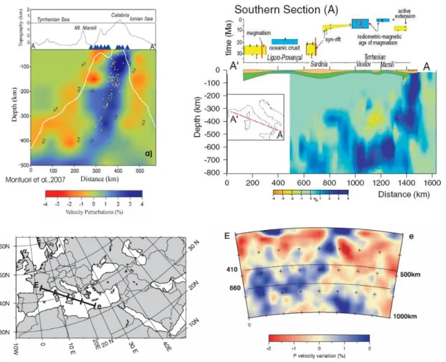
In the last decades, many tomographic studies have been performed to define the seismic velocity field in the crust and upper mantle beneath the Tyrrhenian-Apennine system in order to provide constraints on the geodynamic evolution of the western Mediterranean Sea (e.g., Scarpa, 1982; Spakman, 1990; Amato et al., 1993a, 1993b; Cimini and Amato, 1993; Piromallo and Morelli, 1997; Lucente et al., 1999; Cimini, 1999; Di Stefano et al., 1999; Cimini and De Gori, 2001; Piromallo and Morelli, 2003; Spakman and Wortel, 2004, Montuori et al., 2007). All tomographic models, using teleseismic data (e.g., Amato et al., 1993b) or both regional and teleseismic events reported by International bulletins (e.g., Spakman et al., 1993) highlight a subvertical oceanic slab underneath Calabrian Arc dipping 70°–75° NW down to 400 km depth (figure 1.1.5).

Fig. 1.1.5 – Some tomographies performed using teleseismic data showing the main features of the

subducting Ionian Slab. Faccenna et al., 2001 (left), Piromallo and Morelli, 2003 (centre), Montuori et al., 2007 (right).

Below this depth, a sub-horizontal deflection of the slab is observed jointly with the north-westward shift of the deep seismicity. The subcrustal seismicity, located between 40 and 350 km depth, correlates well with the strong high-velocity anomaly imaged by the tomographies.

Nevertheless, the resolution of the existing tomographies have not allowed an investigation into heterogeneities within the subducting lithosphere, and the absolute values of the velocity field are not so reliable enough use them to make petrological inferences about the mineral phases existing at high pressure and temperature in this geodynamic context. The lack of resolution of the structures and the low reliability of the

(29)

is, however, useful for global seismic modeling of the Earth with a resolution of about 100 km. The lack of these peculiarities strongly limits the use of the tomographies to constrain the geodynamical models and to understand the several processes linked to the plate-margins as the associate volcanism and the hinge zones.

The principal aim of this work is to obtain a high-resolution seismic tomography based on local earthquake data applying the Weighted Average Model method. In this thesis I will show, beside the classic approach used to realize a local earthquake tomography using the tomoDD program (Zhang and Thurber, 2003) in the southern Tyrrhenian Sea, the methodological guideline to realize and apply the WAM method. This method was completely implemented during the PhD study period as necessity to overcome some limits noticed during the taking in place of the DD tomography.

In fact, thanks to the reliability of the WAM, we interpreted the velocity model in the light of mineral phase equilibria governing the progressive dehydration of H2

O-Mg-bearing silicates in the ultramafic portion of the subducted lithosphere giving important insight about the distribution of the mineral phases within the Ionian slab and of the surrounding mantle.

Furthermore, the detail of the WAM allow an accurate identification of the shape of the Ionian slab and the geometry of some bodies around it, down to about 350 km, with a resolution never obtained before.

Finally, in the last chapter, I will show interesting prospective about the WAM method and its further application that will permit to unify several adjacent WAMs to construct a wide velocity model (more than regional scale) which always having an higher reliability and resolution than an conventional large scale tomography.

(30)

(31)

3. Synthetic and Experimental Tests on the “DD”

Tomography of the Southern Tyrrhenian Sea

3.1 Experimental Data

In this work the experimental data employed are the arrival times of the first impulses P and S, relative to the events located in the window 14°30’ E - 17°E and 37°N - 41°N and recorded during the period 1981-2005.

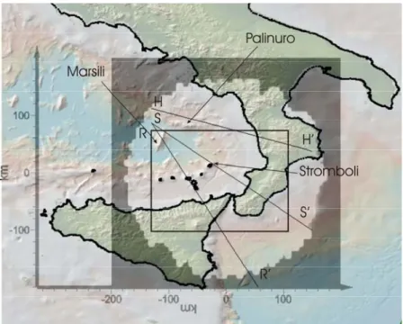
The seismicity of the southern Tyrrhenian region can be subdivided into 2 subsets (figure 3.1.1). The first one contains the shallow seismicity (less than 40 km) produced by the brittle behaviour of the upper portion of the thinned southern Tyrrhenian lithosphere. This is a part of the hinge zone between the African and European plates. This set is elongated in an E-W direction and it runs in latitude from the Sicilian coastline to the Aeolian islands. The second set contains the deep seismicity (down to 500-600 km of depth) mostly located in the eastern part of the southern Tyrrhenian sea between the Aeolian archipelago and the Calabrian coastline. The hypocentres of this set are located in a well developed Wadati-Benioff zone having average dip of 69°-72° and NW polarity, as a result of the subduction of the Ionian lithosphere beneath the Calabrian arc and Tyrrhenian sea.

In this work we used both shallow and deep events to realize a local earthquake tomography in the Southern Tyrrhenian sea using the TomoDD code and then the WAM method.

Fig. 3.1.1 – a) Map of the seismicity of the southern Tyrrhenian region. The blue points mark the shallow

earthquakes (less than 40 km) while the red squares the deep events.

The data set used mainly contains P and S arrival-times taken from the INGV1’s Italian seismicity catalogue (CSI2 and others). We integrated the INGV data set with arrival times, picked out on wave-forms recorded from some temporary arrays. The 1-D model that uses

1

Italian National Institute of Geophysics and Volcanology

(32)

the INGV to locate the Italian events is a simple model with only 3 layers. The mean RMS for the events located in this region is estimated on 0.45 s. The absence of a 1-D optimal model for the Tyrrhenian region and the integration of the arrival times induced us to perform a preliminary re-location of the about 4000 recorded events and the optimization of the 1-D model.

3.1.1ABSOLUTE DATA AND 1-DSTARTING MODEL

The preliminary hypocentral re-location and the optimisation of the initial 1-D Vp and Vs models have been performed by a procedure designed to optimize the hypocentral coordinates, the velocity models and the station residuals by minimizing both the L2 norm

of the residuals travel times and their coherence in the offset domain (Giunta et al., 2004). This technique is derived from the observation that the cinematic forward problem solved for a set of events an unsuitable velocity model produces biases on the travel times which show large coherence intervals in the offset domain.

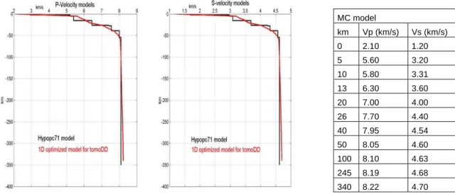
This procedure, initially implemented for HYPOPC71 code (Lee and Lahr, 1985), was adapted to HYPOINVERSE-2000 code (Klein, 2002) to produce an initial 1-D model with constant vertical gradients within the layers, as required by the TomoDD code. The model obtained (that we called MC) represents the initial vertical velocity distribution for the tomographic inversions and for the synthetic and experimental tests (figure 3.1.1). The mean probable error on the epicentral coordinates of the about 4000 re-located events is ~ 2.5 km, whereas on the hypocentral depths it is ~ 4.5 km.

Fig. 3.1.1 – Velocities and depth of the MC model obtained with HYPOPC71 (black) and

HYPOINVERSE-2000 (red).

The events selected from this optimized data set to perform the tomography are recorded by at least 10 stations and marked by RMS (weighted mean square residual) less than 0.50 s after the relocation. The resulting data set refers to 1800 earthquakes (figure 3.1.2a) recorded by on average 16 stations, for a total of 28873 P- and 9990 S- arrival times and relocated with mean RMS = 0.30 s. The total number of stations which recorded the 1800 events was 183 and are moslty located inside the target area.

MC model km Vp (km/s) Vs (km/s) 0 2.10 1.20 5 5.60 3.20 10 5.80 3.31 13 6.30 3.60 20 7.00 4.00 26 7.70 4.40 40 7.95 4.54 50 8.05 4.60 100 8.10 4.63 245 8.19 4.68 340 8.22 4.70

(33)

Fig. 3.2.1 – a) Map of the selected epicentres and stations. b) 3-D view of the hypocentres showing the

down-dip distribution beneath the southern Tyrrhenian sea.

The subcrustal events in this database, located between a depth of 40 and 360 km, are 419. Their hypocentres are concentred within the subducting Ionian lithosphere (figure 3.2.1b).

3.1.2DIFFERENTIAL DATA

We performed several differential data selections to evaluate how much this data set affects the inversion results and if it really improves the reliability of the velocity models. Tests on the importance of the differential data selection will be discussed in section 3.6.3.

In particular, we used several thresholds of some parameters discussed in 2.4 to extract many differential data sets. The least numerous one, obtained fixing the maximum inter-event distance to 10 km, contains 55467 P- and 23992 S- differential times, while the largest, obtained with a threshold of 20 km, encloses 79985 P- and 28370 S- differential times.

(34)

3.2 Inversion Grid

We parameterized the Vp and Vs models assigning velocity values to the nodes of a rectilinear 3-D inversion grid. The continuous velocity field is determined inside each cell using a tri-linear interpolation algorithm (Thurber, 1993). We carried out several inversions using numerous grids with different node positions using both experimental data and synthetic data to perform subsequent tests. The total number of the nodes of each inversion grid is 3276 excluding the marginal nodes. The average lengths of the horizontal grid edges, excluding the boundary nodes, were 310 km and 190 km (figure 3.2.2) whereas the vertical one was 340 km. The average spacing along each direction was 17 km, 38 km and 13 km, respectively. The figure 3.2.1 shows the node positions of the reference inversion grid used for most of the synthetic and experimental tests. This grid has origin of the Cartesian system centred at 38°.667 N and 15°.5 E and the points are at X= -150, -130, 115, 100, 85, 70, 55, 40, 25, 5, 20, 35, 60, 80, 100, 120, 140, 160 km, at Y= 220, -100, -40, 10, 50, 9, 200 km, and at Z= 0, 5, 10, 13, 20, 26, 40, 50, 60, 70, 80, 90, -100, 115, 130, 150, 165, 180, 195, 215, 230, 245, 265, 280, 310, 340 km.

We essentially preferred the anisotropic spacing of the grid along the two horizontal directions with inter-distance ratio between the nodes ~0.5 because previous studies suggested that there is a dominant strike of the deep structures approximately perpendicular to the maximum node density direction. Other authors used similar grids to investigate quasi-2-D structures having strike known a priori (Zhang and Thurber, 2003; Shelly et al., 2006).

Fig. 3.2.2 – Map of the selected epicentres and stations, and inversion grid used for most of the synthetic

and experimental tests. The profiles A-A’ and B-B’ regard the sections discussed in the synthetic and experimental tests.

3.3 Restoration Resolution Test

To perform the synthetic tests we used the real distribution of the stations and the hypocenters located with the MC model. We calculated the travel-times with the 3-D model (figure 3.3.1) resulting from an experimental data inversion (MCS). In these test (both synthetic and experimental ones) we will assess the reliability only for the velocity model of the P-waves. In the sections A-A’ and B-B’ of the MCS Vp model a low velocity body is clearly visible, in the right part of the pictures located approximately beneath the Calabrian arc region. These characteristic bodies are inside the well constrained part of the

(35)

other authors to delimit the well constrained part of the model, e.g. Shelly et al., 2006) but confined in its border area. In this work we called the part of the model characterised by DWS values grater than 50 the investigated volume. Synthetic tests could help to assess the reliability of the geometries obtained, or revel some distortions as smearing effects. Furthermore, just beside the low Vp bodies high values of velocity are visible down to 100 km of depth in the section A-A’ and down to 300 km in B-B’. High velocities of the seismic P-waves are typical in the subducting slabs and we will see in the Chapter 6 that the 3-D shape of the Ionian slab justifies this peculiar geometry.

Fig. 3.3.1 – Map of the selected epicentres and stations, and inversion grid used for the and experimental

test. The profiles A-A’ and B-B’ regard the sections of the MCS velocity model. The red lines limit the portion of the poorly resolved model (DWS < 50).

Starting from the MC model and using the synthetic datawithout adding any noise, the result of the test showed that the information contained in the calculated travel times was able to reconstruct velocity distributions closely matching the MCS model in the volumes where the DWS is greater than 50 (figure 3.3.2 left) and that only in section B-B’ a low Vp

(36)

zone is noticeable not recovered in the MCS. However, this body is outside of the well constrained area and it does not affect the features of the model that we will interpret. We performed the restoration-resolution test (Zhao et al, 1992), consisting in the inversion of the synthetic data perturbed with a random noise having standard deviation equal to the L2

norm of the residuals of the experimental data inversion that in our work is estimated of 0.62 s.

The result of this test (figure 3.3.2 right) highlights the stability of the inverse problem and the ability of the selected data to recover the information contained in a 3-D model with strong lateral heterogeneities.

Fig. 3.3.2 – Synthetic test with exact data (left). Restoration Resolution test (right). The red lines limit the

portion of the poorly resolved model (DWS < 50).

3.4 Dependency of the Velocity Model on the Inversion Grid

To evaluate the dependence of the final velocity model on the nodes position of the inversion grid, we carried out several experimental tests, by rotating, translating and deforming the reference inversion grid.

(37)

Fig. 3.4.1 – Models regarding grids A and B used for the experimental tests. The two horizontal sections

(centre and right) show the plane at a depth of 100 km. Compare the similarity of the velocity patterns within the circled areas The red lines limit the portion of the poorly resolved model (DWS < 50).

Both the inversions show low velocity bodies below the Calabrian arc and the southern Tyrrhenian sea north of the Aeolian archipelago. The part of the models between the Calabrian-Sicilian coastline and the Aeolian islands is characterized by high values of seismic velocity. It is worth noting that the ‘stretching’ of the velocity models due to the anisotropic inversion grids used is clearly visible. Nevertheless, the main features of the velocity distributions are clearly congruent.

The relative standard deviation of the velocity estimates obtained in 15 inversions is ~1% in the volumes around the earthquake hypocentres, but increase up to ~7% in the border of the investigated volumes (characterized by DWS>50). This variability does not change the features of the velocity anomalies having linear dimensions greater than 15-25 km.

3.5 Dependency of the Velocity Model on the Initial Model

In this paragraph we show the models obtained in some tests, carried out to evaluate the influence of the initial model on the final velocity distribution. The experimental data inversions were performed using different starting 1-D and 3-D models. The 3-D models are characterized by the presence of slow and/or fast bodies that simulate the investigable portion of the down-going slab (figure 3.5.2 and 3.5.3).

(38)

In the first test we used an initial model close to MCS (figure 3.5.2 first column) while in the second one a model characterised by high velocity in the volumes where MCS depicts low velocities (figure 3.5.2 second column). Subsequently, we tested an initial model with an intermediate 3-D velocity distribution (figure 3.5.3 first column). In all these tests the experimental data produced 3-D models comparable to the MCS model.

A 1-D model with velocities 1 km/s higher than the MC below a depth of 40 km (figure 3.5.3 second column) led to a velocity distribution similar to that of MCS showing the low influence of the 1-D initial condition on the final velocity model.

Fig. 3.5.2 – Dependency of the tomographic results on the initial models. In the first row 3-D initial

(39)

Fig. 3.5.3 – Dependency of the tomographic results on the initial models. In the first row 3-D and 1-D

initial models are displayed. Below the initial model it is possible to see the vertical sections obtained along the profiles A-A’ and B-B’ . The red lines limit the portion of the poorly resolved model (DWS < 50).

In conclusion, these tests showed that with the selected data set the inverse problem is practically independent of the initial model and always reconstructs the features of the MCS model, even if we observed some biases on the absolute velocity values, especially in the border areas where are depicted important features of the Vp model.

(40)

3.6 Dependency of the Velocity Model on the Experimental Data

Selection Rules

3.6.1DEPENDENCY ON THE ABSOLUTE DATA SELECTION

To assess the dependence of the tomographic model on the data selection procedure we inverted the following data sets: a) the first one includes the events that occurred between 1988 and 2002, having RMS less than 0.5s and at least 10 P-arrival times per event; the total number of selected events was 1492; b) the second one covers the 1981-2005 period, uses the same thresholds of RMS and number of registration per event, for a total of 1800 events selected; c) the last data set contains the events recorded in the 1981-2005 period having at least 10 registrations per event and RMS less than 0.7s; the total number of selected events was 2434. The differential data for all the sets have been determined with the same construction scheme.

Figure. 3.6.1 – DWS distributions relative to the three data sets containing 1428 (left), 1800 (centre) and

2463 (right) events, respectively.

The inversions gave coherent results, however the largest data set, even if it includes data with larger errors, seems to have produced more reliable models, increasing consistently the DWS in many nodes that were poorly constrained by the smaller data set (figure 3.6.1) without dramatically altering the velocity distribution.

3.6.2 DEPENDENCY ON THE DIFFERENTIAL DATA SELECTION

Different differential data sets have been obtained by varying the parameters as the maximum distance between event pair and station, the maximum hypocentral separation between the events of a pair (inter-event distance), the maximum number of neighbors per event and the minimum number of links required to define a neighbour.

Several inversions have been performed for the three absolute data sets assessing the influence of the individuation rules of event pairs on the final velocity model and hypocentral location.

The table 3.6.3.1 illustrates how the size of the differential data set strongly depends on the setting of the input parameters. In this case we highlighted the importance of the maximum inter-event distance threshold during the dataset construction.

(41)

Table. 3.6.2.1 – Table showing the dependence of the size of the differential data set as function of the

inter-event threshold. In the last colon are reported the mean RMS of the events re-located with the absolute and differential data displayed in the table and with the same weighting scheme for all the inversions.

The low spreading of the RMS reported in the table shows that the hypocentral location (and the velocity inversion) are stable with respect to the change of the differential data set. Waldhauser suggests to fix the threshold MAXSEP taking into account the hypocentral incertitude location and starting values of 10 km is considered as reasonable. In our case to fix 10 km as the inter-event distance threshold (two times the incertitude of the hypocentral depth) seems to be the best solution for the largest absolute datasets while for the smallest one seems to be 6 km.

3.6.3 DEPENDENCY ON THE RATIO OF THE ABSOLUTE DATA/DIFFERENTIAL DATA

Subsequently, we tested how much the weighting scheme of TomoDD, between absolute and differential data, could affect the final results.

The authors of the program (Zhang and Thurber) suggest that a good strategy for the iterative procedure is to alternate joint inversions (velocity model and hypocentral location) to simple re-locations. Besides to alternate joint/simple inversions, the authors suggest giving high weight to absolute data in the first steps and to subsequently increase the differential data weights gradually to add more details to the velocity structures determined during the first steps. They affirmed that this strategy gives the smallest location and velocity errors.

The table 3.6.3.1 reports 10 inversion schemes relative to different weighting strategies. In the tests 1, 2 and 3 we generally gave high weight to the differential data in the first steps while in the 4, 5 and 6 tests we used an opposite strategy. In the last 4 tests, we tested the strategy suggested by Thurber and others with mixed weights.

1 NITER WTCTP WTCTS WRCT WDCT WTCD DAMP JOINT

2 1 1 -9 -9 0.1 140 1 1 1 1 -9 -9 0.1 95 0 3 1 1 6 6 1 120 1 1 1 1 6 -9 1 100 0 3 1 1 6 6 10 110 1 1 1 1 6 6 10 100 0

1 10 10 -9 -9 0.1 120 1 2 1 1 -9 -9 0.1 110 1 Number of events maxsep (km) abs. P abs. S dt P dt S mean RMS of the hypocentres 1428 6km 22742 8389 23992 7492 0.125 1428 10km 22742 8389 40063 13021 0.129 1428 20km 22742 8389 78352 26086 0.133 1428 50km 22742 8389 100924 32225 0.138 1800 10km 28873 9990 55467 15239 0.116 1800 15km 28873 9990 72995 22983 0.115 1800 20km 28873 9990 79985 28370 0.119 2463 6km 37159 13802 54409 18092 0.146 2463 10km 37159 13802 61926 20255 0.131 2463 15km 37159 13802 84777 27992 0.139

(42)

3 1 1 6 6 1 170 1

1 1 1 6 -9 1 120 0

3 0.1 0.1 6 6 10 160 1

1 0.1 0.1 6 6 10 100 0

2 0.1 0.1 -9 -9 1 120 1 1 0.1 0.1 -9 -9 1 100 0 2 1 1 -9 -9 1 150 1 2 1 1 6 -9 0.5 120 1 2 1 1 6 6 0.1 120 1 1 1 1 6 6 0.1 100 0

3 0.1 0.1 -9 -9 10 160 1 1 0.1 0.1 -9 -9 10 120 0 1 10 10 -9 -9 1 105 0 3 10 10 6 -9 0.1 130 1 3 0.1 0.1 6 6 10 120 1 1 10 10 8 6 0.1 130 1

2 0.1 0.1 -9 -9 10 160 1 1 1 1 -9 -9 10 90 0 3 1 1 -9 -9 1 135 1 1 1 1 6 -9 1 100 0 3 10 10 6 6 0.1 120 1 1 10 10 8 6 0.1 95 0

2 1 1 -9 -9 10 130 1 1 1 1 -9 -9 10 95 0 3 1 1 -9 6 1 80 1 2 10 10 10 10 1 150 1 2 10 10 6 6 0.1 130 1 1 10 10 6 6 0.1 90 0

3 10 10 -9 -9 0.1 130 1 2 10 10 -9 -9 0.1 120 0 3 1 1 -9 -9 1 130 1 2 1 1 10 10 1 120 1 3 0.1 0.1 8 8 1 130 1 2 0.1 0.1 8 8 1 120 0

1 10 10 -9 -9 1 110 0 2 1 1 -9 -9 10 180 1 2 1 1 -9 -9 1 110 1 2 10 10 6 -9 0.1 160 1 1 10 10 6 6 0.5 140 1 1 10 10 8 6 0.1 100 0

3 1 1 -9 -9 1 170 1