Stochastic Weighted Fractal Networks

RESEARCH OUTPUTS / RÉSULTATS DE RECHERCHE

Author(s) - Auteur(s) :

Publication date - Date de publication :

Permanent link - Permalien :

Rights / License - Licence de droit d’auteur :

Bibliothèque Universitaire Moretus Plantin

Institutional Repository - Research Portal

Dépôt Institutionnel - Portail de la Recherche

researchportal.unamur.be

University of Namur

Stochastic Weighted Fractal Networks

Carletti, Timoteo

Publication date:

2010

Document Version

Early version, also known as pre-print

Link to publication

Citation for pulished version (HARVARD):

Carletti, T 2010 'Stochastic Weighted Fractal Networks'.

General rights

Copyright and moral rights for the publications made accessible in the public portal are retained by the authors and/or other copyright owners and it is a condition of accessing publications that users recognise and abide by the legal requirements associated with these rights. • Users may download and print one copy of any publication from the public portal for the purpose of private study or research. • You may not further distribute the material or use it for any profit-making activity or commercial gain

• You may freely distribute the URL identifying the publication in the public portal ?

Take down policy

If you believe that this document breaches copyright please contact us providing details, and we will remove access to the work immediately and investigate your claim.

Timoteo Carletti

D´epartement de Math´ematique,

Facult´es Universitaires Notre Dame de la Paix 8 rempart de la vierge B5000 Namur, Belgium

[email protected] (Dated: February 1, 2010)

In this paper we introduce new models of complex weighted networks sharing several properties with fractal sets: the deterministic non-homogeneous weighted fractal networks and the stochastic weighted fractal networks. Networks of both classes can be completely analytically characterized in terms of the involved parameters. The proposed algorithms improve and extend the framework of weighted fractal networks recently proposed in [39].

PACS numbers: 89.75.Hc Complex networks, 05.45.Df Fractals, 05.40.-a Stochastic processes

I. INTRODUCTION

Fractal structures are ubiquitous in nature, coast-lines [1], river networks [2, 3], snowflakes [4], grow-ing colonies of bacteria [5–7], mammalian lungs [8–12], mammalian bloody vessels [12], just to mention few of them [50]. But also mankind artifacts can exhibit fractal features, for instance fractal antenna [15] or fluctuations in markets prices [16].

A distinction can be made between mathematical or de-terministic fractals [17] for which a complete geometric description can be provided using simple tools such as ho-motheties, rotations and copying, and random or pseudo fractals [13] found in nature, being the latter character-ized by exhibiting fractal properties, for instance self– similarity, only when statistical averages are computed, because unavoidable fluctuations and errors can alter the regular–geometric patterns. Moreover such scale invari-ance should be limited to a finite range of scale lengths because of physical constraints.

It is worth remarking that some of these physical frac-tals have functionalities, e.g. transportation of gases in mammalian lungs, or charges in fractal antenna, one can thus improve the geometrical description by includ-ing flows and growths constraints. Networks are there-fore the most natural and useful tool to describe such growing complex structures with flows constraints. We thus hereby propose the Stochastic Weighted Fractal Net-works, SWFN for short, a new class of complex networks whose construction is directly inspired by such physical fractal structures.

Starting from the pioneering works of Erd˝os and R´enyi [18], network theory is nowadays a research field in its own [19, 20] and the scientific activity is mainly devoted to construct and characterize complex networks exhibiting some of the remarkable properties of real net-works, scale–free [21], small–world [22], communities [23], weighted links [24–29], just to mention few of them.

In recent years we observed an increasing number of papers were authors proposed models of deterministic (pseudo) fractal networks [30–39] exhibiting scale-free and hierarchical structures. In a limited number of cases,

models presented also a stochastic component [40–43]. The aim of the SWFN hereby introduced, is to provide a framework that could be used to (re)analyze flows on natural fractal structures using standard tools of trans-port theory on networks. Moreover SWFN share with physical fractals several interesting properties, for in-stance the self-similarity or the self-affinity, the presence of hierarchical structures and a stochastic growth pro-cess. Actually this allows us to generalize in a unifying scheme some of the above mentioned models existing in the literature.

The SWFN are constructed via a stochastic process and we are thus able to analytically characterize their topology as a function of the parameters involved in the construction, using expectations obtained construct-ing several replicas.

Let us conclude this introduction with two remarks. First of all we named our models “fractal”networks in-stead of “pseudo fractal”, because some of the topologi-cal properties of SWFN depend on the fractal dimension of some underlying fractal set, whose value ranges all the positive real numbers, without any limitation. Second we rather prefer to talk about “stochastic”networks to em-phasize the stochastic growth process instead of the ran-domness of some topological quantities; let us also stress that in the network theory ”randomness”has a precise meaning that we cannot directly apply to this case.

The paper is organized as follows. In the next section we will introduce and study a deterministic model, that generalize the one proposed in [39], and that will serve as the basic building block to construct the SWFN in Section III. Then we conclude with some possible appli-cations we sum up and draw our conclusions

II. DETERMINISTIC WEIGHTED FRACTAL NETWORK

According to Mandelbrot [17] “a fractal is by definition a set for which the Hausdorff dimension strictly exceeds the topological dimension”. One of the most amazing and interesting feature of fractals is their self-similarity

2

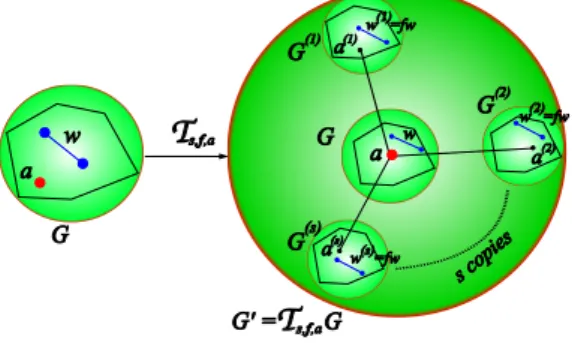
FIG. 1: The map Ts,f ,a. On the left a generic initial graph G with its attaching node a (red on-line) and a generic weighted edge w ∈ G (blue on-line). On the right the new graph G′ obtained as follows: Let G(1)_{, . . . , G}(s)_{be s copies of G, whose} weighted edges (blue on-line) have been scaled respectively by a factor f1, . . . , fs, and let us denote by a(i), for i = 1, . . . , s, the node in G(i)_{image of the labeled node a ∈ G, then link} all those labeled nodes to a ∈ G through edges of unitary weight. The connected network obtained in this way will be by definition the image of G through the map: G′_{= T}

s,f ,a(G).

or self-affinity [44, 45], namely looking at all scales we can find conformal or stretched copies of the whole set; this is actually the idea used to build up fractals as fixed point of Iterated Function Systems [46, 47], IFS for short. Such fractals have a Hausdorff dimension completely charac-terized by the number of copies and the scaling factors of the IFS. Let us observe that in this case this dimension coincides with the so called similarity dimension [47].

Recently, author proposed [39] a new general frame-work aiming to construct weighted netframe-works with some a priori prescribed topology depending on the two main parameters: the number of copies and the scaling fac-tors, hence on the fractal dimension of the “underly-ing”IFS fractal. The aim of this Section is to generalize such construction to obtain a larger class of networks; moreover exploiting the iterative construction we will be able to completely and analytically describe the network topology in terms of node strength distribution, average (weighted) shortest path and (weighted) clustering coef-ficient.

Let us fix a positive integer s > 1 and s real num-bers f1, . . . , fs ∈ (0, 1) and let us consider a (possibly)

weighted network G composed by N nodes, one of which has been labeled attaching node and denoted by a. We then introduce a map, Ts,f ,a, depending on the

parame-ters s, f = (f1, . . . , fs) and on the labeled node a, whose

action on networks is described in Fig. 1.

So starting with a given initial network G0we can

con-struct a family of weighted networks (Gk)k≥0 iteratively

applying the map Ts,f ,a: Gk = Ts,f ,a(Gk−1).

This construction improves the one recently pro-posed [39] by avoiding the introduction of an extra node, moreover it offers a unifying framework where several constructions presented in literature can be included and generalized, e.g. the model presented in [32] with m = 3 can be mapped into to the WFN with s = 3,

f _{= (1, 1, 1), i.e. no weights, and G0 = •. Finally this} deterministic construction will be the basic brick to de-velop the stochastic network introduced in the following Section III.

Given G0and the map Ts,f ,awe are able to completely

characterize the topology of each Gk for k ≥ 1 and also

of the limit network G∞, defined as the fixed point of the

map, Ts,f ,a(G∞) = G∞.

A. Results

The aim of this section is to describe the topology of the graphs Gk for all k ≥ 1 and G∞, by analytically

studying their properties such as the average degree, the node strength distribution, the average (weighted) short-est path and the (weighted) clustering coefficient.

At each iteration step the graph Gkgrows as the

num-ber of its nodes increases according to

Nk = (s + 1)kN0, (1)

being N0the number of nodes in the initial graph, while

the number of edges satisfies

Ek= (s + 1)k(E0+ 1) − 1 , (2)

being E0 the number of edges in G0. Hence in the limit

of large k the average degree is asymptotically given by Ek Nk −→ k→∞ E0+ 1 N0 . (3)

Let us denote the weighted degree of node i ∈ Gk, also

called node strength [25], by ωi(k)=

P jw (k) ij , being w (k) ij

the weight of the edge (ij) ∈ Gk; then using the recursive

construction, we can explicitly compute the total node strength, Wk=Piω

(k)

i , and easily show that

Wk = · 2s F ¡(F + 1) k_{− 1¢ + (F + 1)}k W0 ¸ , (4) being F =Ps

j=1fj. Let us observe that using the

hy-pothesis fj< 1, it trivially follows that F < s, hence we

can conclude that the average node strength goes to zero as k increases: Wk/Nk −→

k→∞0.

B. Node strength distribution.

Let gk(x) denote the number of nodes in Gk that have

strength ω(k)i = x and let us assume g0 to have values in

some finite discrete subset of the positive reals, namely: g0(x) > 0 if and only if x ∈ {x1, . . . , xm} ,

otherwise g0(x) = 0. Using the property of the map

T_{s,f ,a} we get that after k steps of the construction the nodes strengths have been rescaled by a factor fk1

10−6 10−4 10−2 100 102 100 101 102 103 104 x D −1 log 1 0 gk (x )

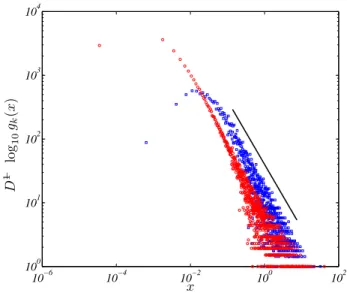
FIG. 2: Node Strengths Distribution. Plot of the renor-malized node strengths distribution D−1_log

10gk(x), where D = −s log s/ log(f1. . . fs). Symbols refer to : ¤ the finite approximation G11 with 3145728 nodes of the WFN with s = 3, f = (1/√2, 1/√3, 1/√5) and G0 =•Á_•|

•; ° the finite approximation G9 with 3359232 nodes of the WFN s = 5, f = (1/√5, 1/√11, 1/√3, 1/√7, 1/√13) and G0 = •−•. The reference line has slope −1, linear best fits (data not shown) provides a slope −1.037 ± 0.04 and R2 _{= 0.798 for ¤ and} −1.00 ± 0.03 and R2= 0.8382 for °.

where the non-negative integers ki do satisfy k1+ · · · +

ks≤ k. Because this can be done in k!/(k1! . . . ks!)

pos-sible different ways, we get the following relation for the node strength distribution for the network Gk:

gk(f1k1. . . fsksx) =

k! k1! . . . ks!

g0(x) with k1+ · · · + ks≤ k .

(5) After sufficiently many steps and assuming that the main contribution arises from the choice k1 ∼ · · · ∼ ks∼ k/s,

we can use Stirling formula to get the approximate dis-tribution (see Fig. 2)

log gk(x) ∼

s log s log(f1. . . fs)

log x , (6)

so the nodes strength distribution follows a power law. Let us observe that in the case of homogeneous scaling, i.e. all fj equal to some f ∈ (0, 1), one can prove [39]

that Eq. (6) reduces to log gk(x) ∼ −df ractlog x where

df ract= − log s/ log f is the fractal dimension of the

un-derlying IFS fractal.

C. Average weighted shortest path.

By definition the average weighted shortest path [20] of the graph Gk is λk= Λk Nk(Nk− 1) , (7) where Λk = X ij∈Gk p(k)ij , (8)

being p(k)ij the weighted shortest path linking nodes i and

j in Gk. Taking advantage of the recursive construction

and adapting the ideas used in [39], we get the following recursive relation for Λk

Λk= (F + 1)Λk−1+ 2s(F + 1)Nk−1Λ(ak−1k−1)+ 2s 2_N2 k−1, (9) where we introduced Λ(ak) k = P i∈Gkp (k)

iak, i.e. the sum of

all weighted shortest paths ending at the attaching node, ak ∈ Gk. We can prove that for large k the asymptotic

behavior of Λ(ak) k is given by Λ(ak) k _k→∞∼ sN0 s − F(s + 1) k_{, (10)}

and thus the recursive relation (9) can be explicitely solved to provide the following asymptotic behavior in the limit of large k (see Fig. 3)

λk −→ k→∞

2s2_{(s + 1)}

(s − F )[(1 + s)2_{− (1 + F )]}. (11)

One can explicitly compute the average shortest path, ℓk, formally obtained by setting f1= · · · = fs= 1 in the

previous formulas (7) and (8). Hence slightly modifying the results presented above we can prove that asymptot-ically we have (see Fig. 4)

ℓk ∼ k→∞ 2s (1 + s) log(s + 1)log Nk N0 , (12)

where growth law of Nkgiven by (1) has been used. Thus

the network grows unbounded with the logarithm of the network size, while the weighted shortest distances stay bounded.

D. Clustering coefficient.

The clustering coefficient [20, 22] of the graph Gk is

defined as the average over the whole set of nodes of the local clustering coefficient c(k)i , namely < ck>= Ck/Nk,

where Ck =Pi∈Gkc

(k) i .

Because of the construction algorithm new triangles are created in the network “boundary”while their number

4 0 1 2 3 4 5 6 7 8 0 0,2 0,4 0,6 0,8 1 1,2 k ˜ λk

FIG. 3: The average weighted shortest path. Plot of the renormalized average weighted shortest path ˜λk versus the iteration number k, where ˜λk = λk(s−F )[(1+s)

2

−(1+F )] 2s2_(s+1) and

F = f1+ · · · + fs. Symbols refer to : ¤ the WFN s = 3, f = (1/√2, 1/√3, 1/√5) and G0 =•Á_•| •; ° the WFN s =5, f = (1/√5, 1/√11, 1/√3, 1/√7, 1/√13) and G0 = •−•; ♦ the WFN s = 2, f = (1/√3, 1/√5) and G0 =•Á_•_•; ∗ the WFN s = 2, f = (1/√3, 1/√5) and G0=•Á_•| •ÂÁ•.

doesn’t change in the inner core, hence the local cluster-ing coefficient, at each step increases just by a factor s+1; thus after k–interactions we will have Ck = (1 + s)kC0,

being C0 =Pi∈G0c

(0)

i the sum of local clustering

coef-ficients in the initial graph. We can thus conclude that the clustering coefficient of the graph is asymptotically given by: < ck> −→ k→∞ C0 N0 . (13)

On the other hand, one can introduce the links val-ues to weigh the clustering coefficient [48], generalizing the previous relation, we can easily prove that weighted clustering coefficientof the graph is asymptotically given by: < γk >= µ 1 + F 1 + s ¶k _C 0 N0 ∼ k→∞ 1 Nk1−d , (14)

where d = log(1+F )_log(1+s), that results smaller than one because of the assumption fj < 1. 100 101 102 103 104 0 1 2 3 4 5 6 7 8 9 10 Nk/N0 ˜ ℓk

FIG. 4: The average shortest path ℓk as a function of the network size(semilog plot). Semilog plot of the renormalized average shortest path ˜ℓk versus the network size Nk, where ˜

ℓk = ℓk(s+1) log(s+1)_2s . Symbols are the same of Fig. 3. The reference line has slope 1. Linear best fits (data not shown) provides a slope 0.970±0.017 and R2_{= 0.9999 for ¤, 0.9654±} 0.05 and R2_{= 0.9997 for °, 0.97 ± 0.02 and R}2_{= 0.9998 for} ♦_{and 1.01 ± 0.03 and R}2_{= 0.9993 for ∗.}

III. STOCHASTIC WEIGHTED FRACTAL NETWORKS

The aim of this section is to present a class of complex weighted networks that grow according to a stochastic process and exhibit self-similar or self-affine structures, hereby named Stochastic Weighted Fractal Networks, for short SWFN, whose construction is directly inspired by the stochastic growth phenomena present in nature. The idea is thus to mimic the growth of fractal structures in nature where “possible errors”could modify regular pat-terns.

So let us hypothesize that the growth process is the result of a stochastic process that selects the actual real-ization, i.e. the number of copies, between a number of different possibilities. Thus at each iteration the number of copies, s, is a stochastic variable distributed accord-ing to some probability distribution function p(s). Once the numerical value for s has been set, s real numbers f1, . . . , fs are drawn according to some probability

dis-tribution function q(f ) with values in (0, 1). Finally a new network is constructed by applying Ts,(f1,...,fs),a to

the actual network: G 7−→

p(s)G (s)_{= T}

s,(f1,...,fs),aG . (15)

simpli-fying working hypothesis that f1 = · · · = fs = α/s, i.e.

q(f ) = δ(f − α/s), for some given and fixed α ∈ (0, 1), but of course the model applies to more general cases.

One can repeat the construction k times and thus ob-tain with probability p(sk) . . . p(s1), starting from a

net-work G0, a new network, denoted by G(sk,...,s1):

G(sk,...,s1)_{= T} sk,(f1(k),...,f (k) sk),a◦ · · · ◦ Ts1,(f1(1),...,f (1) s1),aG0. (16) The network growth results thus a stochastic process, hence we will describe the main topological network mea-sures in terms of expectations obtained repeating several times the construction. Of course we could also consider and compute higher order momenta, but the computa-tions become rapidly cumbersome, and thus we will non present these results except for some simple cases, such as the number of nodes.

A. Results: SWFN

At each step the number of nodes increases with re-spect the present ones, and the exact amount depends on the number of branches drawn. Starting from a net-work containing N0 nodes we get a new network with

N(s1) _{= (1 + s}

1)N0 nodes with probability p(s1).

Iter-ating the construction, after k steps we can obtain with probability p(sk) . . . p(s1) a network with N(sk,...,s1) =

(1 + sk) . . . (1 + s1)N0 nodes. Hence the expected value

for the number of nodes in a network build after k itera-tions, is given by:

< Nk >= X sk,...,s1 p(sk) . . . p(s1)N(sk,...,s1) (17) = X sk p(sk)(1 + sk) X sk−1,...,s1 p(sk−1) . . . p(s1)N(sk−1,...,s1) = (1+ < s >) < Nk−1> , where we denoted by < s >= P skp(sk)sk the

aver-age number of branches. We can thus conclude that the expected number of nodes increases exponentially

< Nk >= (1+ < s >)kN0. (18)

Using similar ideas one can prove that the variance of the

number of nodes increases according to: σ2Nk= N 2 0£(1+ < s >)2+ σs2 ¤k −(1+ < s >)2kN0, (19) where σ2

s is the variance of the distribution of number of

branches.

On the other hand the number of edges can increase, with probability p(sk), in one iteration by E(sk,...,s1) =

(1 + sk)E(sk−1,...,s1)+ sk and thus the expected number

of edges do satisfy

< Ek >= (1+ < s >)k(E0+ 1) − 1 . (20)

These findings are exact in the case of infinitely many replicas, nevertheless numerical simulations presented in Fig. 5 and in Fig. 6 show the good agreement also for finitely many repetitions.

Remark. _{The numerical simulations presented in the} following will be obtained assuming for the branch number a Poisson distribution translated by one, more precisely to avoid a non zero probability of drawing zero branches, we drawn with probabilityp(k) = λk_e−λ_{/k! a non}

nega-tive integerk, and then we set the number of branches to s = k + 1, in this way we will get < s >= λ + 1, σ2_{= λ}

ands ≥ 1.

Of course our findings are more general and do not rely on the particular choice forp(s).

In a similar way we can compute the expected average degree after k steps, < (E/N )k >, and the expected

av-erage node strength after k steps, < (W/N )k >, where

W is the total node strength for the given network real-ization, to get (see Fig. 6):

¿µ E N ¶ k À → k→∞ E0+ 1 N0 and ¿µ W N ¶ k À → k→∞0 . (21) As we did in the previous section, we are able to analyt-ically study other relevant quantities such as the expected value for the weighted shortest path < λk >, defined for

each network realization by (7). More precisely, starting from a network G0 and applying iteratively the above

construction we end up after k iterations with probabil-ity p(sk) . . . p(s1) to a network G(sk,...,s1), we can thus

define the weighted shortest path for the given network realization by λ(sk,...,s1)₌ Λ(sk,...,s1)

(N(sk,...,s1)₎2. Then using the

recursive construction we get:

λ(sk,...,s1) ₌ (Fk+ 1)Λ s_k−1,...,s1_{+ 2s}2 k¡N(sk−1 ,...,s1)¢2 (1 + sk)2¡N(sk−1,...,s1) ¢2 + 2sk(Fk+ 1)Λ sk−1,...,s1 ak N (sk−1,...,s1) (1 + sk)2¡N(sk−1,...,s1) ¢2 = Fk+ 1 (1 + sk)2 λ(sk−1,...,s1)_{+ 2} µ sk sk+ 1 ¶2 +2sk(Fk+ 1) (1 + sk)2 ˆ λ(sk,...,s1)_{, (22)}

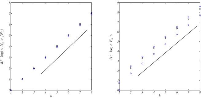
6 1 2 3 4 5 6 7 8 0 1 2 3 4 5 6 7 8 k ∆ −1 log (< N k > /N 0 ) 1 2 3 4 5 6 7 8 0 1 2 3 4 5 6 7 8 9 k ∆ −1 log < Ek >

FIG. 5: Expected values for number of Nodes and number of Edges. Renormalized quantities : ∆−1_{log(< N}

k > /N0) and ∆−1_{log < E}

k > where ∆ = log(1+ < s >). Symbols refer to : ° the SWFN with parameters λ = 4, α = 0.5 and G0 = •−•; ¤ the SWFN with parameters λ = 2, α = 0.5 and G0 =•Á_•|

•; ♦ the SWFN with parameters λ = 3, α = 0.8 and G0 =•ÁÂ • | •. Expectations are obtained over 100 replicas. Left panel, the reference line has slope 1, linear best fits (data not shown) give 0.9998 ± 0.03 R2 _{= 0.9991 for ° and 1.017 ± 0.008 R}2 _{= 0.9999 for ¤, 1.008 ± 0.005 R}2 _{= 1.000 for ♦. Right panel, the} reference line has slope 1, linear best fits (data not shown) give 0.9569 ± 0.06 R2= 0.9988 for °, 1.019 ± 0.03 R2= 0.9997 for ¤_{and 1.06 ± 0.07 R}2 = 0.9955 for ♦. 1 2 3 4 5 6 7 8 0 0.2 0.4 0.6 0.8 1 k < (E /N )k > /D 1 2 3 4 5 6 7 8 0 0.2 0.4 0.6 0.8 1 1.2 1.4 1.6 1.8 2 k < (W /N )k >

FIG. 6: Expected values for the average degree and the average node strength. Renormalized quantities : < (E/N )k> /D where D = (E0+ 1)/N0. Symbols are the same of Fig. 5. Expectations made over 100 replicas.

ˆ

λ(sk,...,s1) _{= Λ}(sk,...,s1)

ak /N

(sk,...,s1)_.

One can finally prove that the expected value for the

average weighted shortest path satisfies the recurrence equation: hλki = hλk−1i ¿ _{1 + F} (1 + s)2 À + 2 * µ _s s + 1 ¶2+ + 2¿ s(1 + F ) (1 + s)2 À Dˆλk E , (23)

where we defined ¿ 1 + F (1 + s)2 À = X k p(k) 1 + Fk (1 + sk)2 , *_µ s s + 1 ¶2+ = X k p(k) µ _s k sk+ 1 ¶2 and ¿ s(1 + F ) (1 + s)2 À = X k p(k)sk(1 + Fk) (1 + sk)2 . (24)

Under the simplifying assumption f1 = · · · = fsk =

α/skwe get Fk= α and thus we can simplify the previous

equations and obtain (see Fig. 7):

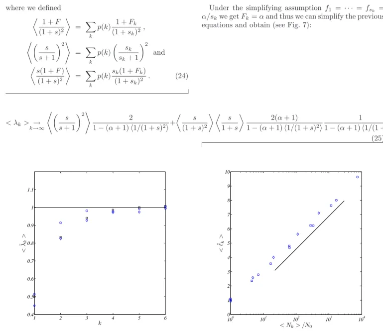
< λk > → k→∞ *_µ s s + 1 ¶2+ 2 1 − (α + 1) h1/(1 + s)2_i+ ¿ s (1 + s)2 À ¿ s 1 + s À 2(α + 1) 1 − (α + 1) h1/(1 + s)2_i 1 1 − (α + 1) h1/(1 + s)i. (25) 1 2 3 4 5 6 0.4 0.5 0.6 0.7 0.8 0.9 1 1.1 k < ˜ λk >

FIG. 7: Expected values for the average weighted shortest path. Renormalized quantities: < ˜λk >= L−1< λk>, where L is the right hand side of Eq. (25). Symbols are the same of Fig. 5. Expectations made over 20 replicas.

One can consider the expected shortest path by formally set all the scaling factors equal to 1 and similar technics allow to conclude that (see Fig. 8)

< ℓk > ∼ k→∞ *_µ s s + 1 ¶2+ ₂ 1 − h1/(s + 1)i 1 log(1+ < s >)log < Nk> N0 . (26) Remark. _{Let us observe that in the case where only} one value ofs is possible, i.e. the probability distribution of the number of branches reduces to a δ–distribution, p(s) = δs,s′, then the above result coincide with the ones

presented for the WFN in Section II.

100 101 102 103 104 0 1 2 3 4 5 6 7 8 9 10 < Nk> /N0 < ˜ ℓk >

FIG. 8: Expected values for the average shortest path as a function of the network size(semilog plot). Semilog plot of the renormalized expected average shortest path < ˜ℓk>=< ℓk> /M versus the network size Nk, where M is the right hand side of Eq. (26). Symbols are the same of Fig. 5. Expectations made over 20 replicas. The reference line has slope 1, linear best fits (data not shown) provides 0.95 ± 0.01 with R2 ₌ 0.9999 for ¤, 0.95 ± 0.07 R2 _{= 0.9968 for ° and 0.98 ± 0.01} R2= 0.9999 for ♦.

IV. CONCLUSIONS

In this paper we proposed a unifying general frame-work for complex weighted netframe-works sharing several properties with fractal sets, the Stochastic Weighted Fractal Networks. This theory, that generalizes to net-works the construction of physical fractals, allows us to build complex networks with a prescribed topology,

8 whose main quantities can be analytically predicted in

terms of expectations and have been shown to depend on the fractal dimension of some underlying fractal; for instance the networks are scale-free, the exponent being the related to the fractal dimension of the underlying IFS. Moreover the SWFN share with fractals, the self-similar or self-affine structure.

These networks exhibit the small-world property. In fact the average shortest path increases logarithmically with the system size; hence it is as small as the average shortest path of a random network with the same number of nodes and same average degree. On the other hand

the clustering coefficient is asymptotically constant, thus larger than the clustering coefficient of a random network that shrinks to zero as the system size increases.

As already observed [39] the self-similarity property of the SWFN make them suitable to model real problems involving some kind of diffusion over the network coupled with local looses of flow, here modeled via the parameters f < 1. Moreover the stochastic growth process allows us to introduce more realism in the construction and thus to extend the applicability domain of our framework to evolving structures.

[1] B.B. Mandelbrot, How Long Is the Coast of Britain? Statistical Self-Similarity and Fractional Dimension, Sci-ence, 156, 3775, (1967), pp. 636-638.

[2] M. Cieplak et al., Models of fractal river basins, J. Stat. Phys., 91, 1/2, (1998), pp. 1.

[3] I. Rodr´ıguez-Iturbe and A. Rinaldo, Fractal River Basins, Cambridge University Press, (2001).

[4] J. Nittman and H.E. Stanley, Non-deterministic ap-proach to anisotropic growth patterns with continuously tunable morphology: the fractal properties of some real snowflakes, J. Phys. A, 20, (1987), pp. L1185.

[5] T. Matsuyama, M. Sogawa and Y. Nakagawa, Fractal spreading growth of Serratia marcescens which produces surface active exolipids, FEMS Microb. Lett., 61, (1989), pp. 243.

[6] H. Fujikawa and M. Matsushita, Fractal Growth of Bacil-lus subtilis on Agar Plates, J. Phys. Soc. Jpn, 58, (1989), pp. 387

[7] H. Fujikawa and M. Matsushita, Bacterial Fractal Growth in the Concentration Field of Nutrient, J. Phys. Soc. Jpn, 60, (1991), pp. 88.

[8] B. Suki, A.-L. Barab´asi, Z. Hantos, F. Pet´ak and H.E. Stanley Avalanches and power–law behaviour in lung in-flation, Nature 368, 615, (1994).

[9] A.-L. Barab´asi, S.V. Buldyrev, H.E. Stanley and B. Suki Avalanches in lung: a statistical mechanical model, Phys. Rev. Lett. 76, (12), 2192, (1996).

[10] H. Kitaoka and B. Suki Branching design of the bronchial tree based on diameter–flow relationship, J. Appl. Phys-iol. 82, 968, (1997).

[11] J.S. Andrade et al. Asymmetric flow in symmetric branched structures, Phys. Rev. Lett. 81, (4), 926, (1998). [12] A. Kamiya and T. Takahashi Quantitative assessments of morphological and functional properties of biological trees based on their fractal nature, J. Appl. Physiol. 102, 2315, (2007).

[13] T. Vicsek, Fractal growth phenomena, World Scientific, (1992).

[14] D. Stauffer and H.E. Stanley, From Newton to Mandel-brot, Springer, (1996).

[15] R. Hohlfeld and N. Cohen Self-similarity and the geomet-ric requirements for frequency independence in Antennae, Fractals, 7, 1, (1999), pp. 7984.

[16] B.B. Mandelbrot, The variation of certain speculative prices, Journ. Business, 36, (1963), pp. 394-419. [17] B.B. Mandelbrot, The Fractal Geometry of Nature, W.H.

Freeman and Company, New York (1982).

[18] P. Erd˝os and A. R´enyi On random graphs, Publ. Math. Debrecen 6, 290, (1959).

[19] R. Albert and A.-L. Barab´asi Statistical mechanics of complex networks, Rev. Mod. Phys. 74, 47, (2002). [20] S. Boccaletti, V. Latora, Y. Moreno, M. Chavez and

D.-H. Hwang Complex networks: Structure and dynamics, Phys. Rep. 424, 175, (2006).

[21] A.-L. Barab´asi and R. Albert Emergence of Scaling in Random Networks, Science 286, 509, (1999).

[22] D.J. Watts and S.H. Strogatz Collective dynamics of ’small-world’ networks, Nature 393, 440, (1998). [23] S. Fortunato Community detection in graphs, Physics

Re-ports, 486, 75, (2010).

[24] S.H. Yook, H. Jeong and A.-L. Barab´asi Weighted evolv-ing networks, Phys. Rev. Lett. 86, (25), 5835, (2001). [25] A. Barrat, M. Barth´elemy, R. Pastor-Satorras and A.

Vespignani. The architecture of complex weighted net-works, Proc. Nat. Acad. Sci. USA 101, 3747, (2004). [26] A. Barrat, M. Barth´elemy and A. Vespignani Modeling

the evolution of weighted networks, Phys. Rev. E 70, 066149, (2004).

[27] D. Zheng, S. Trimper, B. Zheng and P.M. Hui, Weighted scale–free networks with stochastic weight assigments, Phys. Rev. E 67, 040102, (2003).

[28] S.N. Dorogovtsev and J.F.F. Mendes Minimal model of weighted scale–free networks, preprint cond-mat/0408343v2, (2004).

[29] A. Barrat, M. Barth´elemy and A. Vespignani Weighted evolving networks: coupling topology and weight dynam-ics, Phys. Rev. Lett. 92, 22, (2004), pp. 066149. [30] A.-L. Barab´asi, E. Ravasz and T. Vicsek Deterministic

scale–free networks, Physica A, 299, 559, (2001). [31] S.N. Dorogovtsev, A.V. Goltsev and J.F.F. Mendes

Pseudofractal scale–free web, Phys. Rev. E 65, 066122, (2002).

[32] S. Jung, S. Kim and B. Kahng Geometric fractal growth model for scale–free networks, Phys. Rev. E 65, 056101, (2002).

[33] E. Ravasz and A.-L. Barab´asi Hierarchical organization in complex networks, Phys. Rev. E 67, 026112, (2003). [34] Z. Zhang et al., Incompatibily networks as models of

scale–free small–world graphs, Eur. Phys. J.B., 60, (2007), pp. 259.

[35] Z. Zhang et al., Recursive weighted treelike networks, Eur. Phys. J.B., 59, (2007), pp. 99.

[36] Z.Z. Zhang, S.G. Zhou, W.L. Xie, L.C. Chen, Y.Lin, and J.H. Guan, Standard random walks and trapping on the Koch network with scale-free behavior and small-world effect, Phys. Rev. E, 79, (2009), pp. 061113.

[37] J. Guan, Y. Wu, Z. Zhang, S. Zhou, and Y. Wu A unified model for Sierpinski networks with scale-free scaling and small-world effect, Physica A 388, 2571-2578, (2009). [38] Y. Zhang, Z. Zhang, S. Zhou and J. Guan,

De-terministic weighted scale–free small–world networks, arxiv:0910.1140v1 [cond-mat.stat-mech]

[39] T. Carletti and S. Righi, Weighted Fractal Networks, ac-cepted Physica A, (2010).

[40] D.Y.C. Chan, B.D. Hughes, A.S. Leong and W.J. Reed, Stochastically evolving networks, Phys. Rev. E, 68, (2003), pp.066124.

[41] L. Wang, F. Du, H.P. Dai and Y.X. Sun, Random pseud-ofractal scale–free networks with small–world effect, Eur. Phys. J.B, 53, (2006), pp. 361.

[42] L. Wang, H.P. Dai and Y.X. Sun, General random pseud-ofractal networks, J. Phys. A, 40, (2007), pp. 13279. [43] Z. Zhang, S. Zhou, Z. Su, T. Zou and J. Guan Random

Sierpinski network with scale-free small-world and mod-ular structure, Eur. Phys. J. B. 65, 141-147, (2008). [44] B.B. Mandelbrot, Self-affine fractals and fractal

dimen-sion, Physica Scripta, 32, (1985), pp. 257.

[45] B.B. Mandelbrot, in Fractals in Physics, edited by L. Pietronero and E. Tosatti (Elsevier, Amsterdam), (1986), pp. 3.

[46] M. Barnsley, Fractals everywhere, Academic Press Lon-don (1988)

[47] G.A. Edgar, Measure, Topology and fractal geometry, UTM, Springer–Verlag, New York (1990).

[48] J. Saram¨aki, M. Kivel¨a, J.-P. Onnela, K. Kaski and J. Kert´esz Generalizations of the clustering coefficient to weighted complex networks, Phys. Rev. E 75, 027105, (2007).

[49] M¨akinen, V. Himmeli, a free software package for visualizing complex networks, available at http://www.artemis.kll.helsinki.fi/himmeli.

[50] The interested reader could find many more example in the beautiful books [13, 14].