RESEARCH OUTPUTS / RÉSULTATS DE RECHERCHE
Author(s) - Auteur(s) :
Publication date - Date de publication :
Permanent link - Permalien :
Rights / License - Licence de droit d’auteur :
Bibliothèque Universitaire Moretus Plantin
Institutional Repository - Research Portal
Dépôt Institutionnel - Portail de la Recherche
researchportal.unamur.be
University of Namur
Weighted Fractal Networks
Carletti, Timoteo; Righi, Simone
Published in:
Physica A
Publication date:
2010
Document Version
Early version, also known as pre-print
Link to publication
Citation for pulished version (HARVARD):
Carletti, T & Righi, S 2010, 'Weighted Fractal Networks', Physica A, vol. 389, pp. 2134-2142.
General rights
Copyright and moral rights for the publications made accessible in the public portal are retained by the authors and/or other copyright owners and it is a condition of accessing publications that users recognise and abide by the legal requirements associated with these rights. • Users may download and print one copy of any publication from the public portal for the purpose of private study or research. • You may not further distribute the material or use it for any profit-making activity or commercial gain
• You may freely distribute the URL identifying the publication in the public portal ?
Take down policy
If you believe that this document breaches copyright please contact us providing details, and we will remove access to the work immediately and investigate your claim.
corresponding author (*) [email protected]
(Dated: July 6, 2009)
In this paper we define a new class of weighted complex networks sharing several properties with fractal sets, and whose topology can be completely analytically characterized in terms of the involved parameters and of the fractal dimension. The proposed framework defines an unifying general theory of fractal networks able to unravel the hidden mechanisms responsible for the emergence of fractal structures in nature.
PACS numbers: 64.60.aq Complex Networks, 89.75.Fb Structures and organization in complex systems, 89.75.Da Scale-free networks, 05.45.Df Fractals
I. INTRODUCTION
Complex networks have recently attracted a growing interest of scientists from different fields of research, mainly because complex networks define a powerful framework for describing, analyzing and modeling real systems that can be found in nature and/or society. This framework allows to conjugate the micro to the macro abstraction levels: nodes can be endowed with local dynamical rules, while the whole network can be though to be composed by hierarchies of clusters of nodes, that thus exhibits aggregated behavior.
The birth of graph theory is usually attributed to L. Euler with his seminal paper concerning the “K¨onigsberg bridge problem”(1736), but it is only in the 50’s that network theory started to develop autonomously with the pioneering works of Erd˝os and R´enyi [4]. Nowaday network theory defines a research field in its own [5, 6] and the scientific activity is mainly devoted to construct and characterize complex networks exhibiting some of the remarkable properties of real networks, scale–free [7], small–world [8], communities [9], just to mention few of them.
In a series of recent papers [1–3] authors proposed a new point of view by constructing networks exhibiting scale-free structures following ideas taken from fractal construction, e.g. Koch curve or Sierpinski gasket. The aim of the present paper is to generalize these latter constructions and to define a unifying theory, hereby named Weighted Fractal Networks, WFN for short, whose networks share with fractal sets several interesting properties, for instance the self-similarity.
The WFN are constructed via an explicit algorithm and we are able to completely analytically characterize their topology as a function of the parameters involved in the construction. We are thus able to prove that WFN exhibit the “small–world”property, i.e. slow (logarithmic) increase of the average shortest path with the network size, and large average clustering coefficient. Moreover the probability distribution of node strength follows a power law whose exponent is the Hausdorff (fractal) dimension of the “underlying”fractal, hence the WFN are scale–free.
WFN also represent an explicitely computable model for the renormalization procedure recently applied to complex networks [10–12].
The paper is organized as follows. In the next section we will introduce the model and we outline the similarities with fractal sets. Section III is aimed to present the analytical characterization of such networks also supported by dedicated numerical simulations. After the presentation of a straightforward generalization of the present theory in Section IV, we conclude by presenting a possible application of WFN to the study of fractal structures emerging in nature.
II. THE MODEL
According to Mandelbrot [13] “a fractal is by definition a set for which the Hausdorff dimension strictly exceeds the topological dimension”. One of the most amazing and interesting feature of fractals is their self-similarity, namely looking at all scales we can find conformal copies of the whole set. Starting from this property one can provide rules to build up fractals as fixed point of Iterated Function Systems [14, 15], IFS for short, whose Hausdorff dimension is completely characterized by two main parameters, the number of copies s and the scaling factor f of the IFS. Let us observe that in this case this dimension coincides with the so called similarity dimension [15], df ract= − log s/ log f .
The main goal of this paper is to generalize such ideas to networks, aimed at constructing weighted complex networks [20] with some a priori prescribed topology, that will be described in terms of node strength distribution,
2
FIG. 1: The action of Ts,f,a on a generic network G. We schematically represents the action of Ts,f,a on the initial attaching
node a, its images a(1), . . . , a(s) and the new one a′ (red on-line) and on a generic weighted edge w ∈ G and its images
w(1), . . . , w(s)(blue on-line).
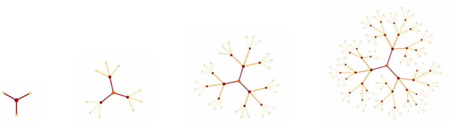
FIG. 2: The “Sierpinski” WFN, s = 3, f = 1/2 and G0 is composed by a single node. From the left to the right G1, G2, G3
and G4. Gray scale (color on-line) reproduces edges weights: the darker the color the larger the weight. The dimension of the
fractal is log 3/ log 2 ∼ 1.5850. Visualization was done using Himmeli software [16].
average (weighted) shortest path and average (weighted) clustering coefficient, depending on the two main parameters: the number of copies and the scaling factor [21]. Moreover taking advantage of the similarity with the IFS fractals, some topological properties of the networks will depend on the fractal dimension of the IFS fractal.
Let us fix a positive real number f < 1 and a positive integer s > 1 and let us consider a (possibly) weighted network G composed by N nodes, one of which has been labeled attaching node and denoted by a. We then define a map, Ts,f,a, depending on the two parameters s, f and on the labeled node a, acting on networks as follows:
Let G(1), . . . , G(s) be s copies of G, whose weighted edges has been scaled by a factor f . For i = 1, . . . , s
let us denote by a(i) the node in G(i) image of the labeled node a ∈ G, then link all those labeled nodes
to a new node a′ through edges of unitary weight. The connected network obtained linking the s copies
G(i)to the node a′ will be by definition the image of G through the map: G′= T
s,f,a(G) (see Fig. 1).
So starting with a given initial network G0 we can construct a family of weighted networks (Gk)k≥0 iteratively
applying the previously defined map: Gk:= Ts,f,a(Gk−1).
Because of its general definition, the map Ts,f,aimproves the constructions recently proposed in [1–3], allowing us
to consider all possible IFS fractals in a unified scheme. For the sake of completeness we present numerical results for two WFN : the Sierpinski one (see Fig. 2) and the Cantor dust (see Fig. 3).
Given G0 and the map Ts,f,awe are able to completely characterize the topology of each Gk and also of the limit
network G∞, defined as the fixed point of the map: G∞ = Ts,f,a(G∞). Thus the WFN undergo through a growth
process strictly related to the inverse of the renormalization procedure [10, 11]; at the same time G∞will be infinitely
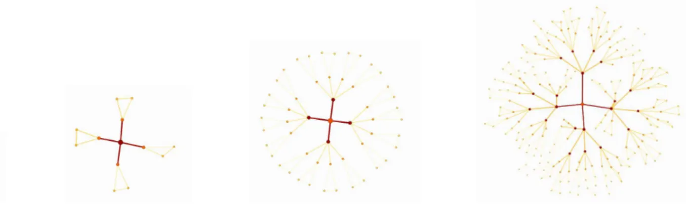
FIG. 3: The “Cantor dust” WFN, s = 4, f = 1/5 and G0 is a triangle. From the left to the right G0, G1, G2 and G3.
Gray scale (color on-line) reproduces edges weights: the darker the color the larger the weight. The dimension of the fractal is log 4/ log 5 ∼ 0.8614. Visualization was done using Himmeli software [16].
III. RESULTS
The aim of this section is to characterize the topology of the graphs Gk for all k ≥ 1 and G∞, by analytically
studying their properties such as the average degree, the node strength distribution, the average (weighted) shortest path and the average (weighted) clustering coefficient.
At each iteration step the graph Gk grows as the number of its nodes increases according to
Nk= skN0+ (sk− 1)/(s − 1) , (1)
being N0 the number of nodes in the initial graph, while the number of edges satisfies
Ek = skE0+ s(sk− 1)/(s − 1) , (2)
being E0 the number of edges in the graph G0. Hence in the limit of large k the average degree is finite and it is
asymptotically given by Ek Nk −→ k→∞ s + E0(s − 1) 1 + (s − 1)N0 . (3)
Let us denote the weighted degree of node i ∈ Gk, also called node strength [18], by ω(k)i =
P jw (k) ij , being w (k) ij
the weight of the edge (ij) ∈ Gk; then using the recursive construction, we can explicitly compute the total node
strength, Wk =Piω (k)
i , and, provided sf 6= 1, easily show that
Wk= 2s1 − (sf ) k
1 − sf + (sf )
kW 0.
Because f < 1, we trivially find that the average node strength goes to zero as k increases: Wk/Nk −→ k→∞0.
A. Node strength distribution.
Let gk(x) denote the number of nodes in Gk that have strength ωi(k) = x and let us assume g0 to have values in
some finite discrete subset of the positive reals, namely:
g0(x) > 0 if and only if x ∈ {x1, . . . , xm} ,
otherwise g0(x) = 0. Using the property of the map Ts,f,awe straightforwardly get gk(x) = sgk−1(x/f ) provided [22]
x 6= s and x 6= f s + 1, from which we can conclude that for all k:
4 −40 −3 −2 −1 0 1 1 2 3 4 5 6 7 log10x lo g1 0 g14 (x ) 1 2 3 4 5 6 7 8 9 0 0.5 1 1.5 2 2.5 3 3.5 k λk
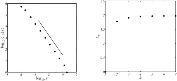
FIG. 4: The “Sierpinski” WFN, s = 3, f = 1/2 and G0is formed by one initial node. Left panel, the node strength distribution
for G14, a 2391484 nodes network; the reference line has slope − log 3/ log 2 ∼ 1.585, a linear best fit (data not shown) provides
a slope −1.59 ± 0.03 and R2= 0.9997. Right panel, average weighted shortest path for Gk, k ∈ {1, . . . , 9}. The horizontal line
represents the asymptotic value predicted by (9).
−80 −6 −4 −2 0 2 1 2 3 4 5 6 log10x log 1 0 g1 0 (x ) 1 2 3 4 5 6 7 0 0.5 1 1.5 2 2.5 k λk
FIG. 5: The “Cantor dust” WFN, s = 4, f = 1/5 and G0is made by a triangle. Left panel, node strength distribution for G10
composed by 873813 nodes; the reference line has slope − log 4/ log 5 ∼ −0.861, a linear best fit (data not shown) provides a slope −0.865 ± 0.015 and R2= 0.9998. Right panel, average weighted shortest path for Gk, k ∈ {1, . . . , 7}. The horizontal line
represents the asymptotic value predicted by (9).
This implies than the node strengths are distributed according to a power law with exponent df ract= − log s/ log f ,
that equals the fractal dimension of the fractal obtained as fixed point of the IFS with the same parameters s and f . In fact defining xik= fkxi we get:
log gk(xik) = k log s + log g0(xi)
= log s
log f log xik+ log g0(xi) − log s log f log xi, namely gk(x) ∼ C/xdf rac (see left panels of Fig. 4 and Fig. 5).
λk= Λk Nk(Nk− 1), (5) where Λk = X ij∈Gk p(k)ij , (6)
being p(k)ij the weighted shortest path linking nodes i and j in Gk.
To simplify the remaining part of the proof it is useful to introduce Λ(ak)
k =
P
i∈Gkp
(k)
iak, i.e. the sum of all weighted
shortest paths ending at the attaching node, ak ∈ Gk. One can prove (see Appendix A 1) that for large k the
asymptotic behavior of Λ(ak) k is given by Λ(ak) k k→∞∼ N0(s − 1) + 1 (1 − f )(s − 1)s k−1. (7)
Using the construction algorithm and its symmetry one can prove (see Appendix A 2) that Λksatisfies the recursive
relation
Λk= sf Λk−1+ 2s[(s − 1)Nk−1+ 1][Nk−1+ f Λ(ak−1k−1)] , (8)
that provides the following asymptotic behavior in the limit of large k (see right panels of Fig. 4 and Fig. 5) λk = Λk Nk(Nk− 1) −→ k→∞ 2(s − 1) (1 − f )(s − f ). (9)
We can also compute the average shortest path, ℓk, formally obtained by setting f = 1 in the previous formulas (5)
and (6). Hence slightly modifying the results presented in the Appendix A 2 we can prove that asymptotically we have ℓk ∼ k→∞2 µ k − s s − 1 ¶ ∼ k→∞ 2 log slog Nk, (10)
where the last relation has been obtained using the growth law of Nk given by (1) (see Fig. 6).
Thus, as previously stated, the network grows unbounded but with the logarithm of the network size, while the weighted shortest distances stay bounded.
C. Average clustering coefficient.
The average clustering coefficient [6, 8] of the graph Gk is defined as the average over the whole set of nodes of
the local clustering coefficient c(k)i , namely < ck >= Ck/Nk, where Ck = Pi∈Gkc(k)i . Because of the construction
algorithm the number of possible triangles, hence the local clustering coefficient, at each step increases by a factor s; thus after k iterations we will have Ck = skC0, being C0 the sum of local clustering coefficients in the initial graph.
We can thus conclude that the clustering coefficient of the graph is asymptotically given by: < ck> −→ k→∞ s − 1 s < c0> N0 (s − 1)N0+ 1 . (11)
On the other hand, one can use edges’ values to weight the clustering coefficient [19]; hence generalizing the previous relation, we can easily prove that the average weighted clustering coefficient of the graph is asymptotically given by:
< γk > ∼ k→∞ s − 1 f s < γ0> N0 (s − 1)N0+ 1 fk ∼ k→∞ 1 N1/df ract k , (12)
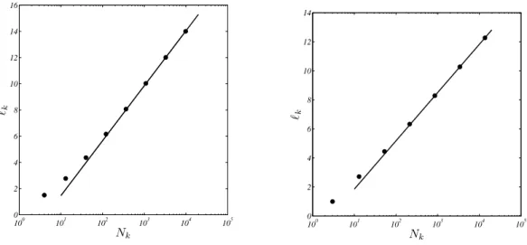
6 100 101 102 103 104 105 0 2 4 6 8 10 12 14 16 Nk ℓk 100 101 102 103 104 105 0 2 4 6 8 10 12 14 Nk ℓk
FIG. 6: The average shortest path ℓk as a function of the network size (semilog graph). Left panel, the “Sierpinski” WFN,
s = 3, f = 1/2 and G0is formed by one initial node. Right panel the “Cantor dust” WFN, s = 4, f = 1/5 and G0 is made by
a triangle. The reported straight lines have slopes 2/ log s and numerically confirm the asymptotic theoretical prediction (10).
FIG. 7: The non–homogeneous “Cantor dust” WFN, s = 4, f1 = 1/2, f2 = 1/3, f3 = 1/5, f4 = 1/7 and G0 is formed by a
triangle. From the left to the right G0, G1, G2 and G3. Gray scale (color on-line) reproduces edges weights: the darker the
color the larger the weight. Visualization was done using Himmeli software [16].
IV. NON–HOMOGENEOUS WEIGHTED FRACTAL NETWORKS
The aim of this section is to slightly generalize the previous construction to the case of non–homogeneous scaling factors for each subnetwork G(i). So given an integer s > 1 and s real numbers f
1, . . . , fs∈ (0, 1), we modify the map
Ts,f,aby allowing a different scaling for each edge weight according to which subgraph it belongs to: if the edge w(j),
image of w ∈ G, belongs to G(j), then w(j)= fjw.
Let us remark that the former construction of Section II is a particular case of the latter, once we take f1= · · · =
fs= f ; we nevertheless decided for a sake of clarity, to present it before, because the computations involved in this
latter general construction could have hidden the simplicity of the underlying idea. We hereby present some results for the non–homogeneous “Cantor dust”WFN (see Fig. 7).
Using the recursiveness of the algorithm we can once again completely characterize the topology of the non-homogeneous WFN, moreover only the weighted quantities will vary with respect to the non-homogeneous case. For instance, a straightforward, but cumbersome, generalization of the computations presented in the previous Sections and in the Appendices A 1 and A 2 allows us to prove that the average weighted shortest path exhibits the following asymptotic behavior (see right panel of Fig. 8)
λk −→
k→∞
2s2(s − 1)
(s − F )(s2− F ), (13)
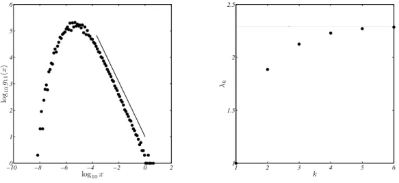
−100 −8 −6 −4 −2 0 2 1 2 3 4 log10x log 1 0 g1 1 (x ) 1 2 3 4 5 6 1 1.5 2 k λk
FIG. 8: The non-homogeneous “Cantor dust” WFN, s = 4, f1= 1/2, f2= 1/3, f3= 1/5, f4= 1/7 and G0is made by a triangle.
Left panel, node strength distribution for G11composed by 3495253 nodes; the reference line has slope s log s/ log(f1f2f3f4) ∼
−1.0370 and numerically confirms the relation (15). Right panel, average weighted shortest path for Gk, k ∈ {1, . . . , 6}. The
horizontal line represents the asymptotic value predicted by (13).
Let g0(x) denote the number of nodes with node strength equal to x in the initial network G0; then after k steps of
the algorithm, all nodes strengths will be rescaled by a factor fk1
1 . . . fsks, where the non-negative integers kido satisfy
k1+ · · · + ks= k. Because this can be done in k!/(k1! . . . ks!) possible different ways, we get the following relation for
the node strength distribution for the network Gk:
gk(f1k1. . . f ks s x) = k! k1! . . . ks! g0(x) with k1+ · · · + ks= k . (14)
After sufficiently many steps and assuming that the main contribution arises from the choice k1∼ · · · ∼ ks∼ k/s, we
can use Stirling formula to get the approximation (see left panel of Fig. 8) log gk(x) ∼
s log s log(f1. . . fs)
log x . (15)
V. CONCLUSIONS
In this paper we introduced a unifying framework for complex networks sharing several properties with fractal sets, hereby named Weighted Fractal Networks. This theory, that generalizes to graphs the construction of IFS fractals, allows us to build complex networks with a prescribed topology, whose main quantities can be analytically predicted and have been shown to depend on the fractal dimension of the IFS fractal; for instance the networks are scale–free with exponent the fractal dimension. Moreover the weighted fractal networks share with IFS fractals, the self-similarity structure, and are explicitely computable examples of renormalizable complex networks.
These networks exhibit the small–world property. In fact the average shortest path increases logarithmically with the system size (10), hence it is small as the average shortest path of a random network with the same number of nodes and same average degree. On the other hand the clustering coefficient is asymptotically constant (11), thus larger than the clustering coefficient of a random network that shrinks to zero as the system size increases.
The self-similarity property of the weighted fractal networks makes them suitable to model real problems involving generic diffusion over the network coupled with local looses of flow, here modeled via the parameter f < 1. For instance one can think of electrical grids or mammalian lungs, where current or air, flows through power lines or bronchi–bronchioles, submitted to looses of power, or air vessels’ section reduction. In all these cases the induced topology, namely a good choice of f and s, allows any two random nodes, final power users or alveoli, to be always at finite weighted distance, whatever their physical distance is, and thus to be able to transport current or air in finite time.
8
Appendix A: Appendix 1. Computation ofΛ(ak)
k
Let ak be the attaching node of the graph Gk. Let us define Λ(akk) =
P
i∈Gkp
(k)
iak, i.e. the sum of all weighted
shortest paths to ak. Then using the recursive property and the symmetry of the map Ts,f,ak we can easily obtain a
recursive relation for Λ(ak)
k :
Λ(ak)
k = sf Λ
(ak−1)
k−1 + sNk−1,
where Nk−1 is the number of nodes in Gk−1. This recursion can be easily solved to get for all k ≥ 1
Λ(ak) k = (sf ) k−1Λ(a1) 1 + 1 − fk−1 1 − f (s − 1)N0+ 1 s − 1 s k−1− s s − 1 (sf )k−1− 1 sf − 1 ,
from which we can conclude, because f < 1, that Λ(ak)
k exhibits the asymptotic behavior given by (7).
2. Computation of Λk
Starting from the definition of the sum of all weighted shortest paths (6), the recursive construction and its symmetry
we can decompose the sum Λk into three terms:
Λk = s X ij∈G(1)k p(k)ij + s(s − 1) X i∈G(1)k ,j∈G(2)k p(k)ij + 2s X i∈G(1)k p(k)iak (A1)
where the first contribution takes into account all paths starting from and arriving to nodes belonging to the same subgraph, that using the symmetry can be chosen to be G(1)k . The second term takes into account all the possible paths where the initial point and the final one belong to two different subgraphs, and still using the symmetry we can set them to G(1)k and G(2)k and multiply the contribution by a combinatorial factor s(s − 1). Finally the last term is the sum of all paths arriving to the attaching node ak; once again the symmetry allows us to reduce the sum to only
one subgraph, say G(1)k , and multiply the contribution by 2s.
The first term in the right hand side of (A1) can be easily identified with X
ij∈G(1)k
p(k)ij = f Λk−1.
By construction, each shortest path connecting two nodes belonging to two different subgraphs, must pass through the attaching node, hence using p(k)ij = p(k)iak+ p(k)akj the second term of (A1) can be split into two parts:
X i∈G(1)k ,j∈G(2)k p(k)ij = X i∈G(1)k p(k)iakNk(2)+ X j∈G(2)k p(k)akjNk(1),
where Nk(i)denotes the number of nodes in the subgraph G(i)k . Using the symmetry of the construction, the previous relation can be rewritten as
X i∈G(1)k ,j∈G(2)k p(k)ij = 2N (1) k X i∈G(1)k p(k)iak.
The last term of (A1) can be related to Λ(ak−1)
k−1 by observing that each path arriving at ak must pass through a(i)k
for some i ∈ {1, . . . , s}, thus X i∈G(1)k p(k)iak = X i∈G(1)k (p(k) ia(1)k + p (k) a(1)k ak ) = Nk(1)+ X i∈G(1)k p(k) ia(1)k = Nk(1)+ f Λ(ak−1) k−1 , (A2)
[1] Z. Zhang, J. Guan, L. Chen, M. Yin and S. Zhou, Novel scale-free small-world networks from Koch curves, preprint (2008), cond-mat.stat-mech/0810.3313v1.
[2] Z. Zhang, S. Zhou, Z. Su, T. Zou and J. Guan, Random Sierpinski network with scale-free small-world and modular
structureEur. Phys. J. B., 65, (2008), pp. 141-147.
[3] J. Guan, Y. Wu, Z. Zhang, S. Zhou and Y. Wu, A unified model for Sierpinski networks with scale-free scaling and
small-world effect, Physica A, 388, (2009), pp. 2571-2578
[4] P. Erd˝os and A. R´enyi, On random graphs, Publ. Math. Debrecen 6, (1959), pp. 290.
[5] R. Albert and A.-L. Barab´asi, Statistical mechanics of complex networks, Rev. Mod. Phys., 74, (2002), pp. 47.
[6] S. Boccaletti, V. Latora, Y. Moreno, M. Chavez and D.-H. Hwang, Complex networks: Structure and dynamics, Phys. Rep, 424, (2006), pp. 175.
[7] A.-L. Barab´asi and R. Albert, Emergence of Scaling in Random Networks, Science 286, (1999), pp. 509. [8] D.J. Watts and S.H. Strogatz, Collective dynamics of ’small-world’ networks, Nature, 393, (1998), pp. 440. [9] S. Fortunato, Community detection in graphs, preprint arXiv:0906.0612v1 [physics.soc-ph] 3 Jun 2009. [10] C. Song, S. Havlin and H.A. Makse, Self-similarity of complex networks, Nature 433, (2005), pp. 392.
[11] C. Song, S. Havlin and H.A. Makse, Origin of fractality in the growth of complex networks, Nature Physics 2, (2006), pp. 275.
[12] F. Radicchi, A. Barrat, S. Fortunato and J.J. Ramasco, Renormalization flows in complex networks, preprint arxiv:/physics.soc-ph/0811.2761v1, (2008).
[13] B.B. Mandelbrot, The Fractal Geometry of Nature, W.H. Freeman and Company, New York (1982). [14] M. Barnsley, Fractals everywhere, Academic Press London (1988)
[15] G.A. Edgar, Measure, Topology and fractal geometry, UTM, Springer–Verlag, New York (1990).
[16] V. M¨akinen, Himmeli, a free software package for visualizing complex networks, available at http://www.artemis.kll.helsinki.fi/himmeli.
[17] T. Carletti, Stochastic Weighted Fractal Networks, preprint (2009).
[18] A. Barrat, M. Barth´elemy, R. Pastor-Satorras and A. Vespignani, The architecture of complex weighted networks, Proc. Natl. Acad. Sci. USA 101, (2004), pp. 3747.
[19] J. Saram¨aki, M. Kivel¨a, J.-P. Onnela, K. Kaski and J. Kert´esz, Generalizations of the clustering coefficient to weighted
complex networks, Phys. Rev. E, 75, (2007), pp. 027105.
[20] We hereby present the construction for undirected networks, but it can be straightforwardly generalized to directed graphs as well.
[21] A straightforward generalization will be presented in section IV. See also [17] where the present construction will be generalized as to include a stochastic iteration process.
[22] Without loose of generality we can assume that for all integers i, j ∈ {1, . . . , m} and k > 0 we have fkx
j 6= xi and
fk(f x