HAL Id: tel-03179093
https://tel.archives-ouvertes.fr/tel-03179093
Submitted on 24 Mar 2021HAL is a multi-disciplinary open access archive for the deposit and dissemination of sci-entific research documents, whether they are pub-lished or not. The documents may come from teaching and research institutions in France or abroad, or from public or private research centers.
L’archive ouverte pluridisciplinaire HAL, est destinée au dépôt et à la diffusion de documents scientifiques de niveau recherche, publiés ou non, émanant des établissements d’enseignement et de recherche français ou étrangers, des laboratoires publics ou privés.
learning techniques
Felix Gontier
To cite this version:
Felix Gontier. Analysis and synthesis of urban sound scenes using deep learning techniques. Acoustics [physics.class-ph]. École centrale de Nantes, 2020. English. �NNT : 2020ECDN0042�. �tel-03179093�
T
HESE DE DOCTORAT DE
L'ÉCOLE
CENTRALE
DE
NANTES
ECOLE DOCTORALE N°602 Sciences pour l'Ingénieur Spécialité : Acoustique
Analyse et synthèse de scènes sonores urbaines par approches
d’apprentissage profond
Thèse présentée et soutenue à Nantes, le 15 décembre 2020
Unité de recherche : UMR6004, Laboratoire des Sciences du Numérique de Nantes (LS2N)
Par
Félix GONTIER
Rapporteurs avant soutenance :
Dick Botteldooren Professeur, Ghent University, Belgique Gaël Richard Professeur, Télécom Paris, Palaiseau
Composition du Jury :
Président : Catherine Marquis-Favre Directrice de recherche, ENTPE, Vaulx-en-Velin
Examinateurs : Romain Serizel Maître de conférences, Université de Lorraine, Vandœuvre-lès-Nancy Dir. de thèse : Jean-François Petiot Professeur des universités, École Centrale de Nantes
Co-dir. de thèse : Catherine Lavandier Professeure des universités, Université de Cergy-Pontoise Encadrant : Mathieu Lagrange Chargé de recherche, École Centrale de Nantes
First and foremost, I would like to thank the members of my thesis com-mittee, Catherine Marquis-Favre, examiner and jury president, Dick Bottel-dooren and Gael Richard, reviewers, and Romain Serizel, examiner, for the interest they demonstrated towards my work and their insightful comments. I am deeply grateful to my thesis director Jean-François Petiot, as well as Catherine Lavandier and Mathieu Lagrange who supervised my work. Each of them brought complementary expertise which was instrumental to the completion of my thesis, along with exceptional availability and help-fulness. In particular, Mathieu Lagrange guided my work with unparalleled open-mindedness, enthusiasm, and patience.
For providing me with a rich research environment, I am also grateful to the Sims team at Laboratoire des Sciences du Numérique de Nantes, as well as members of the Cense project. The diverse backgrounds and area of interest of the people I encountered in the past three years opened my eyes to numerous new perspectives that were important to my development as a researcher. Among them, special thanks to Pierre Aumond for his invaluable assistance on acoustic and psychoacoustic scientific fields.
I express my utmost appreciation to Vincent Lostanlen, who took the time to provide in-depth commentary on the present manuscript with con-siderable expertise.
I would like to thank Ranim Tom for his help in dataset curation, as well as the many students at École Centrale de Nantes who participated in listening experiments.
Lastly, my thoughts go to my family and friends, whose continued sup-port largely contributed to making this doctoral study a pleasant experience.
Acknowledgements 2 Table of contents 4 List of figures 7 List of tables 13 List of publications 15 Introduction 16
1 Perception of urban sound environments 22
1.1 Soundscape quality . . . 23
1.2 Content-based assessment of soundscape quality . . . 24
1.3 Acoustic indicators . . . 26
1.4 Framework for soundscape quality prediction with deep learning 30 2 Automatic annotation of perceived source activity for large controlled datasets 34 2.1 Introduction . . . 35
2.2 Subjective annotations . . . 38
2.2.1 Motivation . . . 38
2.2.2 Listening test corpus . . . 39
2.2.3 Subjective annotation procedure . . . 41
2.3 Perceptual validation of simulated acoustic scenes . . . 45
2.3.1 Simulated scene construction . . . 45
2.3.2 Scenario generation . . . 47
2.4 Indicator for the automatic annotation of simulated datasets . 51 2.4.1 Formulation . . . 51
2.4.2 Evaluation . . . 57
3 Prediction of the perceived time of presence from sensor measurements using deep learning 63 3.1 Introduction . . . 63
3.2 Controlled dataset . . . 65
3.3 Architectures . . . 66
3.3.1 Convolutional neural network . . . 66
3.3.2 Recurrent decision process . . . 68
3.3.3 Training procedure . . . 70
3.4 Evaluation . . . 73
3.4.1 Source presence predictions . . . 73
3.4.2 Application to the estimation of subjective attributes . 75 3.4.3 Application to sensor data in Lorient . . . 77
4 Domain adaptation techniques for robust learning of acoustic predictors 81 4.1 Introduction . . . 83
4.1.1 Design of deep learning architectures . . . 83
4.1.2 Transfer learning . . . 84
4.1.3 Pretext tasks for audio . . . 86
4.1.4 Localized embeddings . . . 88
4.2 Audio representation learning from sensor data . . . 90
4.2.1 Large dataset of sensor measurements . . . 90
4.2.2 Encoder architecture . . . 91
4.2.3 Supervised pretext tasks . . . 93
4.2.4 Unsupervised pretext task . . . 95
4.3 Presence prediction with transfer learning . . . 98
4.3.1 Local controlled dataset . . . 98
4.3.2 Source presence prediction architecture . . . 101
4.3.3 Evaluation of model performance on target sound en-vironments . . . 103
4.4 Experiments . . . 106
4.4.1 Evaluation of the transfer learning approach . . . 106
4.4.2 Content of simulated training datasets . . . 109
4.4.3 Quantity of downstream task training data . . . 111
5 Acoustic scene synthesis from sensor features 116 5.1 Introduction . . . 118
5.3 Experimental protocol . . . 121 5.3.1 Considered approach . . . 121 5.3.2 Dataset . . . 121 5.3.3 Baselines . . . 122 5.3.4 Phase recovery . . . 125 5.3.5 Objective metrics . . . 126 5.4 Deterministic approach . . . 129 5.4.1 Architecture . . . 129 5.4.2 Evaluation . . . 131 5.5 Generative approach . . . 135
5.5.1 Generative adversarial networks . . . 135
5.5.2 Generator architecture . . . 137
5.5.3 Critic architecture . . . 141
5.5.4 Training process . . . 143
5.5.5 Evaluation . . . 144
Conclusion 146
A Scene level parameters for acoustic scene simulation 149 B Comparison of perceptual responses between recordings and
1 Overview of research topics where deep learning approaches are investigated in the current work. . . 18 1.1 Example of sensor network developped as part of the CENSE
project, and noise map (Lden) for the city of Lorient. . . 27 1.2 Possible configurations for the prediction of soundscape
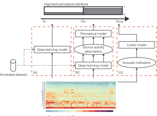
qual-ity attributes from sensor data. (a) Direct prediction of high-level attributes. (b) Prediction of intermediary source activ-ity descriptors and application of a perceptual model. (c) Approach developed in the literature, derivation of acoustic indicators and linear modeling of perceptual attributes. . . 31 2.1 Overview of the scene simulation process from scenarios and
a database of isolated source samples. . . 36 2.2 Map of the soundwalks and 19 recording locations in the 13th
district of Paris presented in [1]. Sound levels shown on the soundwalk path are interpolated from measurements at each location. . . 37 2.3 Time of presence of sources estimated by the indicator
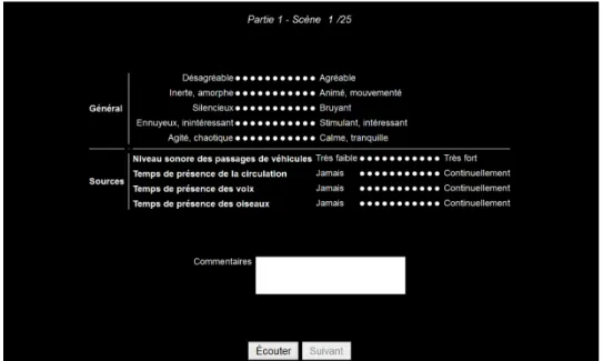
pro-posed in Section 2.4 for the 75 simulated scenes in the listening test corpus. . . 41 2.4 Screenshot of the Python interface presented during the
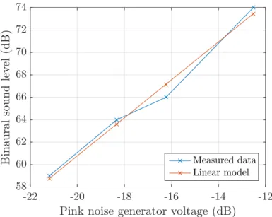
lis-tening test. . . 42 2.5 Measurements and linear model of the playback sound level of
Beyerdynamics DT-990 Pro headphones (Lhead) as a function of input pink noise electrical level (log(Vgen)). . . 44
2.6 Biplot of the principal components analysis of average as-sessments for the 5 high-level perceptual attributes on the 6 recorded and 19 replicated scenes (n=25). Arrows indicate differences between projections of assessments for the recorded (base) and replicated (head) scenes of each location. For the P1 location ellipses show the distributions of individual as-sessments. . . 47 2.7 Biplot of the principal components analysis of average
as-sessments for the 5 high-level perceptual attributes on the 6 recorded and 19 replicated scenes (n=25). . . 48 2.8 Biplot of the principal components analysis of average
assess-ments for the 5 high-level perceptual attributes on the 75 sim-ulated scenes (n=75). Assessments of simsim-ulated scenes (active individuals) are projected as dots, and recorded and replicated scenes (supplementary individuals) are projected as crosses. . 49 2.9 Lowest equal-loudness contour (dB SPL) in the ISO 226:2003
norm, taken as an absolute threshold of hearing curve. . . 52 2.10 Spectra of harmonic and noise components in polyphonic
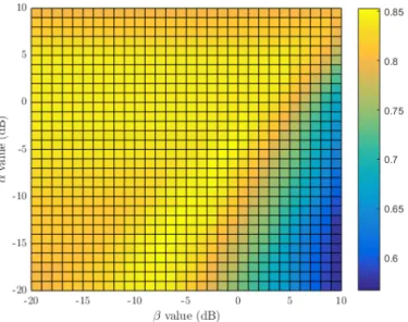
sig-nals for different signal to noise ratios and noise colors. The harmonic component is perceptually masked only in (c). . . . 54 2.11 Average Pearson correlation coefficient between the proposed
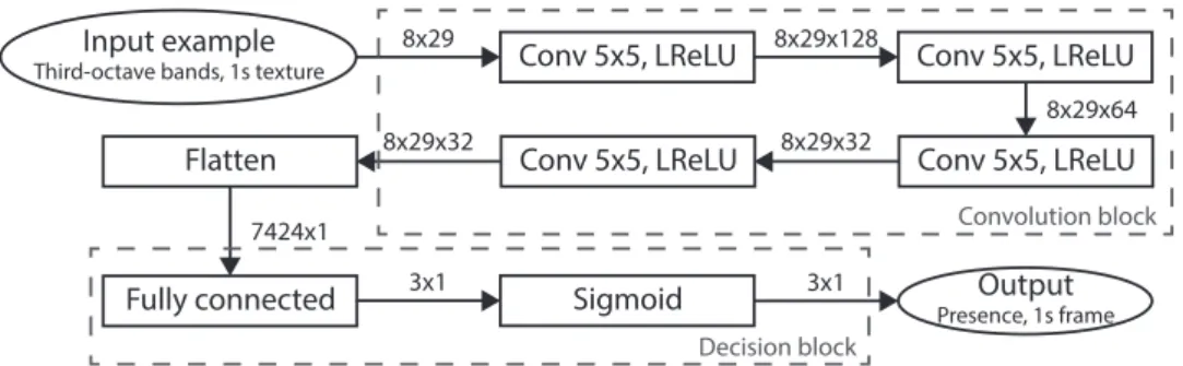
time of presence estimation ˆTs(α, β) and subjective annota-tions as a function of α and β values. . . 56 3.1 Architecture of the proposed convolutional neural network for
source presence prediction in 1 s textures of third-octave fast measurements. . . 66 3.2 Information flow in a gated recurrent unit cell. The update
(blue) and reset (red) gates filter information from the current input xtand recurrent state ht−1to compute the hidden state ht. . . 70 3.3 Architecture of the proposed recurrent neural network for
source presence prediction in 1 s textures of third-octave fast measurements (unrolled view). Parameters are shared along all timesteps. . . 71 3.4 Extraction of 1 s textures xnwith 875 ms overlap from
third-octave measurements, input sequentially to the recurrent neu-ral network. . . 72 3.5 Evolution of training and validation losses of the convolutional
3.6 Maps of predictions by the convolutional (top) and recurrent (bottom) networks of the time of presence of traffic (left), voices (middle), and birds (right), for data collected by the Cense network on the 20th of August 2020 between 22h and 22h10. . . 78 4.1 Typical architecture design of deep discriminative or
encoder-decoder approaches. Similar encoder architectures are rele-vant to solve a variety of related tasks, whereas the decision or decoder is task-specific. . . 84 4.2 General framework of transfer learning approaches. An
en-coder is trained to solve a pretext task on a large dataset, and the same encoder architecture in the downstream task is initialized with obtained optimal parameters architecture, in order to stabilize training with few labeled examples. . . 85 4.3 Map of sensors implemented as part of the Cense network in
Lorient. The SpecCense dataset is composed of data from the 16 sensors shown in blue. . . 90 4.4 Proposed encoder architecture to extract information from 1 s
third-octave texture frames. This architecture is common to all studied models in a transfer learning setting. . . 92 4.5 Proposed architectures for the SensorID and Time pretext
tasks models. . . 93 4.6 Evolution of training and validation losses for the SensorID
and Time pretext task models. . . 95 4.7 Encoder-decoder architecture proposed to solve the Audio2Vec
pretext task by predicting a third-octave texture frame from context texture frames. . . 96 4.8 Decoder architecture proposed to solve the Audio2Vec pretext
task. . . 97 4.9 Evolution of the training and validation losses of the
Au-dio2Vec model trained on sensor data. . . 97 4.10 Comparison of the construction process for the TVBUniversal,
TVBCense and SpecCense datasets in this study. . . 100 4.11 Decision architecture for the downstream task of source
pres-ence prediciton. . . 102 4.12 Histograms of the maximum difference in time of presence
4.13 Comparison of presence prediction accuracy in EvalLorient recorded scences between models trained on the TVBUniver-sal and TVBCense simulated datasets. . . 110 4.14 Performance of models trained with a limited number of
simu-lated scenes evaluated on source presence accuracy in Lorient recordings. . . 112 4.15 Performance of models trained with a limited isolated samples
database evaluated on source presence accuracy in Lorient recordings. . . 114 5.1 Proposed spectral approach to waveform reconstruction from
third-octave spectrograms. A deep learning architecture out-puts an estimation of the fine-band spectrogram, which an iterative phase recovery algorithm inverts to waveform audio. 121 5.2 Frequency response of third-ocrave filters in the [20Hz−12500Hz]
range (a), and weights of the associated pseudoinverse matrix (b). . . 123 5.3 Average power spectrum of acoustic scenes in the DCASE2017
development dataset and its reconstruction by the pseudoin-verse transform (a). The estimation error resembles a saw-tooth waveform due to flat estimations within filter band-widths (b). . . 124 5.4 Proposed architecture to refine estimations of fine-band
spec-trograms obtained by application of the third-octave trans-form pseudoinverse. A convolutional neural network outputs corrections added to the input estimation to produce the pre-diction. . . 129 5.5 Example of spectrograms generated with the pseudoinverse
baseline (b) and the proposed CNN (c). The CNN corrects discontinuities at third-octave filter cutoff frequencies, but does not produce fine structure. . . 132 5.6 Average spectra of normalized audio extracts in datasets of
en-vironmental sounds (DCASE2017 task 1), clean speech (Lib-riSpeech) and music (GTZAN). . . 132 5.7 Box plots of the distributions of spectral centroids in sound
scenes of the DCASE2017 dataset, separated by labels of type of sound environment (n=108). . . 134
5.8 Original framework of generative adversarial networks. A gen-erator architecture synthesizes examples from input random vectors. A discriminator is tasked to identify generated ex-amples from real exex-amples in the dataset, and both models are trained jointly in a minimax setting. An additional input optionally conditions synthesis. . . 136 5.9 Proposed generator approach, where separate deep neural
net-works estimate parts of the fine-band magnitude spectrogram corresponding to each third-octave filter. Combining contri-butions from the subnetworks produces the final estimation, and ensures that gradients in subnetworks are not affected by large magnitude differences across frequencies. . . 138 5.10 Example of transposed convolution layer that performs the
parametric upsampling of an input representation, here with an upsampling factor (fractional stride) of 2 and kernel size 2 × 2 . . . 139 5.11 Architecture of individual subnetworks in the generator model.
9 transposed convolution layers upsample the input third-octave spectrogram into an estimation of the fine-band spec-trogram. A random component is introduced with dropout during both learning and evaluation. The number of channels C in hidden layers is a function of the number of frequency bins associated with the third-octave filter inverted by the network. . . 139 5.12 Number of frequency bins in the bandwidth of third-octave
fil-ters and number of channels allocated to corresponding sub-networks in the generator architecture. Both quantities are doubled with each octave. . . 140 5.13 Architecture of the critic model rating the realism of patches
in generated and real fine-band spectrograms. . . 142 B.1 Biplot of the principal components analysis of average
as-sessments for the 5 high-level perceptual attributes on the 6 recorded and 19 replicated scenes (n=25). Arrows indicate differences between projections of assessments for the recorded (base) and replicated (head) scenes of each location. For the P3 location ellipses show the distributions of individual as-sessments. . . 152
B.2 Biplot of the principal components analysis of average as-sessments for the 5 high-level perceptual attributes on the 6 recorded and 19 replicated scenes (n=25). Arrows indicate differences between projections of assessments for the recorded (base) and replicated (head) scenes of each location. For the P4 location ellipses show the distributions of individual as-sessments. . . 153 B.3 Biplot of the principal components analysis of average
as-sessments for the 5 high-level perceptual attributes on the 6 recorded and 19 replicated scenes (n=25). Arrows indicate differences between projections of assessments for the recorded (base) and replicated (head) scenes of each location. For the P8 location ellipses show the distributions of individual as-sessments. . . 154 B.4 Biplot of the principal components analysis of average
as-sessments for the 5 high-level perceptual attributes on the 6 recorded and 19 replicated scenes (n=25). Arrows indicate differences between projections of assessments for the recorded (base) and replicated (head) scenes of each location. For the P15 location ellipses show the distributions of individual as-sessments. . . 155 B.5 Biplot of the principal components analysis of average
as-sessments for the 5 high-level perceptual attributes on the 6 recorded and 19 replicated scenes (n=25). Arrows indicate differences between projections of assessments for the recorded (base) and replicated (head) scenes of each location. For the P18 location ellipses show the distributions of individual as-sessments. . . 156
2.1 Mean differences of perceptual assessments (resp. Pleasant-ness, LiveliPleasant-ness, Overall LoudPleasant-ness, Interest, CalmPleasant-ness, Time of presence of Traffic, Voices, and Birds) between recorded and replicated sound scenes. Significant differences as per a Wilcoxon signed-rank test are shown in bold (n=23, p<0.05) 45 2.2 Pearson’s correlation coefficients between perceptual attributes
averaged over participants, resp. Pleasantness, Liveliness, Overall Loudness, Interest, Calmness, Time of presence of Traffic, Voices, and Birds (n=100, *: p<0.05, **: p<0.01) . . 50 2.3 Pearson’s correlation coefficients between physical and
percep-tual (resp. Pleasantness, Liveliness, Overall Loudness, Inter-est, Calmness, Time of presence of Traffic, Voices, and Birds) indicators (n = 92). . . 58 2.4 Performance of baseline models for pleasantness prediction. . 60 3.1 Performance of the predictions of source presence by deep
learning models trained with binary ground truth labels ˆTs(αopt, βopt). Presence metrics in % are computed for n=68800 1 s frames
and time of presence metrics on n=200 45 s scenes. (TP: true positive, TN: true negative, FP: false positive, FN: false neg-ative) . . . 74 3.2 Pearson’s correlation coefficients between the time of
pres-ence estimated by averaging prespres-ence labels predicted by the proposed deep learning model over time, and subjective an-notations obtained during the listening test. (n=94) . . . 75 3.3 Quality of pleasantness predictions on the listening test corpus
using deep learning models to predict source presence com-pared to ground truth labels. The corpus is split in three parts: the 6 recorded scenes (Rec.), the 19 replicated scenes (Rep.), and the 75 scenes with simulated scenarios (Sim.). . . 77
4.1 Contents of the isolated samples database from which simu-lated scenes in the TVBCense dataset are generated. . . 100 4.2 Source presence prediction accuracy (%) of models with
en-coder parameters pre-trained on pretext tasks compared to learning from scratch. The three metrics are respectively the accuracy on the TVBCense evaluation subset, the standard accuracy on the EvalLorient corpus, and the accuracy modi-fied with label confidence on the EvalLorient corpus. . . 107 4.3 Time of presence prediction root mean squared errors on a
[0-1] scale yielded by predictions of proposed models on Lorient recordings (n=30). . . 109 5.1 Evaluation metrics for examples synthesized with the
pro-posed CNN compared to the pseudoinverse baseline, in terms of reconstruction error (resp. signal to reconstruction ratio, log-spectral distance, perceptual similarity metric) and incep-tion score. Statistics are computed on the DCASE2017 eval-uation dataset (n=1620). Results shown in bold for specific metrics are not statistically different from the best performing system (p<0.05). . . 130 5.2 Signal-to-reconstruction ratio obtained by the proposed CNN
in comparison to the pseudoinverse baseline, as a function of sound environment types in the DCASE2017 evaluation dataset (n=108). . . 133 5.3 Performance of the proposed Ad-SBSR generative approach
compared to the convolutional network (CNN) in Section 5.4, pseudoinverse estimations, and the AdVoc generative baseline. Metrics are evaluated on the DCASE2017 evaluation dataset (n=1620). Results shown in bold for specific metrics are not statistically different from the best performing system (p<0.05).144 A.1 Scene level parameters to generate quiet street environments. 149 A.2 Scene level parameters to generate noisy street environments. 150 A.3 Scene level parameters to generate very noisy street
environ-ments. . . 150 A.4 Scene level parameters to generate park environments. . . 150 A.5 Scene level parameters to generate square environments. . . . 150
Publications dans des revues d’audience internationale
à comité de lecture
• Gontier, F., Lavandier, C., Aumond, P., Lagrange, M. and Petiot, J.-F. (2019). Estimation of the perceived time of presence of sources in urban acoustic environments using deep learning techniques. Acta Acustica united with Acustica, 105(6), 1053-1066
Communications à des congrès internationaux à comité
de sélection et actes publiés
• Gontier, F., Lagrange, M., Lavandier, C., and Petiot, J.-F. (2020). Privacy aware acoustic scene synthesis using deep spectral feature in-version. In 2020 IEEE International Conference on Acoustics, Speech and Signal Processing (ICASSP)
• Gontier, F., Aumond, P., Lagrange, M., Lavandier, C., and Petiot, J.-F. (2018). Towards perceptual soundscape characterization using event detection algorithms. In Workshop on Detection and Classification of Acoustic Scenes and Events (DCASE 2018)
Following the ever-increasing expansion of large cities observed in the last decades, almost 75% of European citizens currently live in urban areas. De-spite being an important component of the quality of life, the sound environ-ment is barely taken into account in the design of those areas. This has led to an important increase of noise pollution [2], which is responsible for several public health issues [3, 4, 5]. In order to mitigate current hazards and to be able to propose new ways that would incorporate the sound modality in the urban planning process, there is an important need to rigorously monitor and gather information about the acoustic environment in urban areas.
Subsequently, monitoring sound environments has become an active field of research, with studies mainly investigating noise assessment and reduc-tion applicareduc-tions. In particular, such is the objective of the 2002/49/CE directive, which requires large European cities to maintain publicly available noise maps [6]. Beyond noise reduction applications, we believe that a de-velopment is needed in order to better characterize and control urban sound environments, by modeling and predicting their impact on the quality of life of urban residents and passers-by. To do so, it is necessary to measure sound environments, and infer meaningful information to communicate to citizens and influence the design of urban areas.
In terms of measuring sound environments, the recent advent of the In-ternet of Things (IoT) has enabled the development of large-scale acoustic sensor networks [7, 8]. Several projects have implemented such networks to monitor urban sound environments, where indicators describing the acoustic content are continuously measured and stored on servers to be processed into relevant quantities. Many of these projects are developed in the con-text of noise assessment studies, with improving predictive noise maps as the primary objective. For example, in the RUMEUR network, 45 sensors continuously gather acoustic information in Paris [9]. In addition, several short-term measurement campaigns specifically refine assessments of aircraft noise. The project also includes a study on graphical representations and
tography of sound environments to better communicate information about their quality to both citizens and administrative parties. The DYNAMAP European project [10] further investigates the potential of low-cost sensor networks in monitoring sound environments of large cities. The developed approach implements a limited number of sensors at important locations of road infrastructures throughout the target cities of Rome and Milan. The network aims at capturing the diversity of traffic conditions in the city, in-cluding traffic density, road type, and weather conditions. The gathered data corrects estimations of predictive sound propagation models to produce maps of short-term noise level variations [11]. The Cense project, to which the present work is applied, proposes a different approach where dense sen-sor grids are implemented in the main districts and streets of Lorient [12]. The sensor network comprises a larger number of low-cost sensors compared to previous studies. Part of the project focuses on data assimilation be-tween predictive models and the spatially dense sensor measurements, with a study on the uncertainties of emission-propagation models. In addition to traditional noise maps, continuously recording informative acoustic data enables the study of more comprehensive approaches to the characterization of sound environments. In order to produce multimodal noise maps easily in-terpretable by the citizens, part of the project is thus dedicated to assessing the perceptual quality of measured sound environments by both residents and passers-by. To this aim, the soundscape approach is prevalent in re-cent studies on the perception of sound environments [13]. In this approach, soundscape quality can be modeled efficiently from the perceived activity of sources on short time periods. Continuous measurements in dense sensor networks should allow the prediction of these quantities of interest, in order to propose detailed short-term maps of sound quality.
Relatedly, recent developments in signal processing have resulted in new efficient tools to model audio signals. Deep learning methods now achieve state-of-the-art results in sound event detection and sound scene classifi-cation. The growing Detection and Classification of Acoustic Sounds and Events (DCASE) community specifically investigates this range of appli-cations, and proposes a recurring challenge on several related tasks1. Some studies have also successfully applied deep learning approaches to monitoring sound environments in the context of large-scale acoustic sensor networks. For example, the SONYC project [14] implements a low-cost sensor network in New York City and develops automatic methods for urban sound tag-ging [15]. Large collected measurement datasets also enable techniques such
Privacy-aware sensor data Sensor network Waveform synthesis Source presence prediction
Figure 1: Overview of research topics where deep learning approaches are investigated in the current work.
as unsupervised representation learning for environmental audio [16]. This dissertation focuses on two contributions, that build on recently proposed deep learning techniques to i) predict perceptual attributes and ii) synthesize acoustic scenes from sensor data, as shown in Figure 1. We believe that the scientific advances in these two domains will allow to better inform citizens and city administrators about sound environments, by communicat-ing easily interpretable information inferred from acoustic sensor networks.
Deep learning approaches to infer perceptual attributes of environmental sounds, either describing high-level properties (e.g. pleasant, lively) or the activity of sound sources, remain largely unexplored. The first contribution of this thesis is thus to propose an original approach using deep learning techniques to predict descriptors of perceived sound quality from sensor data. This includes the design of sufficiently large datasets and their annotation in terms of relevant underlying quantities describing the content of sound environments. In this context, recent studies in psychoacoustics identify the perceived activity of sources of interest as relevant descriptors.
Chapter 1 first establishes a summary of previous studies on the per-ception of environmental sounds and soundscape quality. After reviewing acoustic indicators that can be considered to represent perceptual quanti-ties in published models, the potential of deep learning architectures in the estimation of high-level perceptual attributes is discussed. Specifically, the proposed original approach introduces predictions of perceived source pres-ence from such architectures in models developed on large-scale studies on urban soundscape perception.
The information content recorded by sensors is subject to privacy reg-ulations. Some applications enforce this constraint by obfuscating speech in voice activity segments obtained with source separation algorithms [17].
Instead, the Cense network anonymizes recorded data by directly measuring spectral sound levels [18]. The information content of measurements is insuf-ficient to recover waveform audio with fully identifiable sound sources, and thus to manually annotate extracts for the desired task. Chapter 2 discusses the interest of sound scene simulation tools for automatic annotation of large datasets. The developed methodology allows the simulation of diverse sound scenes by combining extracts of isolated source occurrences according to re-alistic scenarios extrapolated from a corpus of annotated recordings. A lis-tening experiment compares perceptual assessments of simulated scenes to results from the literature. An indicator is then proposed that models the saliency of a given source with respect to all others, from separated source contributions available in simulated scenes. This indicator is associated to the perceived presence of sources of interest in case of active listening of the sound environment by passers-by. Evaluation of the proposed annotation is done against state-of-the-art acoustic indicators, with respect to subjective assessments obtained in the listening test.
In Chapter 3, the developed indicator automatically annotates a large dataset of simulated scenes on the perceived presence of sources of interest. Two trained models, including convolutional and recurrent architectures, are able to predict source presence in synthetic data with high accuracy. Nonetheless, experiments evidence the incompleteness of simulated scenes with respect to sound environments of the application. In particular, the taxonomy of sound sources and associated spectral patterns in simulation processes may limit the adaptability of models to sound sources specific to target environments.
Chapter 4 addresses those limitations by localizing deep learning models to sound environments measured by the Cense sensor network. To do so, transfer learning approaches infer relevant information from large amounts of unlabeled sensor data in pretext tasks. Informative latent audio repre-sentations learned with these methods enable the training of low-complexity architectures predicting the perceived source presence. For this purpose, a second corpus of simulated sound scenes is constructed from on-site record-ings of isolated source occurrences. The proposed experiments compare the relevance of latent audio representations obtained with two discriminative tasks relying on sensor metadata as well as an unsupervised regressive task. Evaluations done on a corpus of annotated recordings gathered in the target sound environments show that localizing simulated data highly contributes to prediction accuracy. Transfer learning and self-supervision further im-proves the effectiveness of architectures trained on simulated sound corpora with limited domain correspondence, data quantity, or diversity. The
pro-posed approach of perceived source presence prediction is adapted to the target in vivo sound environments, although future work remains regard-ing its potential embeddregard-ing into low-cost sensors and its integration to the Geographic Information System (GIS) of the sensor network.
The second contribution aims at producing artificial sound environments that are conditioned with spectral information issued from the sensor net-work. Listening to waveform audio examples associated to sensor measure-ments is useful to provide citizens and urban planners with reference sound scenes illustrating noise maps. In some sensor networks, for instance the SONYC project, waveform audio is directly recorded and stored on secure servers. However, this is not always possible nor desirable due to regula-tions on privacy constraints. In the Cense project, sensor measurements sufficiently degrade the information content so that no waveform audio with intelligible speech can be retrieved [18]. This is also detrimental to the identification of other sound sources in reconstructed audio. In recent liter-ature, deep learning architectures are successfully applied to the synthesis of speech (vocoders) and musical (musical synthesizers) signals. However, few approaches are applied to environmental sound synthesis, which con-tain complex polyphonies as well as diverse spectral signatures associated to sound source contributions. Thus, the second part of this thesis focuses on proposing deep learning models to synthesize plausible sound scenes that correspond to privacy-aware sensor measurements. Sound synthesis being a difficult task, the present work aims at proposing a preliminary study on original approaches to solve issues specific to environmental scenes process-ing. The developed methods thus require significant future work in order to achieve production-ready sound scene synthesis from sensor network mea-surements.
The use of deep generative models to synthesize plausible waveform audio from privacy-aware sensor data is investigated in Chapter 5. Two spectral approaches are considered where a magnitude spectrogram is reconstructed from measured third-octave sound levels, and phase information is recov-ered using iterative algorithms to obtain a waveform signal. Specifically, the first proposed architecture deterministically refines estimations from a data-independent baseline by learning a priori information from a dataset of acoustic scenes. The second proposed architecture upsamples log-frequency spectral representations, and is trained in an adversarial setting to enforce both the realism and the fidelity of generated spectra. The models are eval-uated against deep and non-deep baselines available in the literature using spectral and waveform reconstruction metrics, as well as objective perceptual metrics and automatic classification performance.
We believe that those technical contributions will allow better citizen information and soundscape design in urban areas. The prediction of per-ceptual source activity descriptors is satisfying for the target environment, even if the proposed design and evaluation paradigms should be replicated in other urban areas. The availability of privacy-aware measurements through dense acoustic sensor networks allows exposing useful information about ur-ban sound environments, and deep learning approaches are a promising av-enue of research to do so.
The task of sound scene synthesis being inherently difficult, many under-lying problems are still open in the deep learning community. The contribu-tion developed in this thesis focuses on architectures enforcing invariance of regression loss functions to important variations in the magnitude of envi-ronmental sound spectra across frequencies. While experiments demonstrate the usefulness of the proposed approach, much work is still required to fully understand and tackle the fascinating problem of high-rate audio synthesis with deep learning paradigms.
Perception of urban sound
environments
The soundscape approach is prevalent in recent studies to qualify and quantify the perception of sound environ-ments. This chapter reviews recent literature on the sub-ject, including the characterization of soundscape quality by standardized perceptual dimensions and their relation to the activity of sound sources. In the context of con-tinuous acoustic monitoring with sensor networks, these perceptual quantities can be efficiently approximated by acoustic indicators.
A framework is then proposed where such indicators are replaced by deep learning architectures. Specifically, the task of estimating the perceived time of presence of sources is formulated as an tractable problem of binary presence prediction on small temporal frames, related to event detection and classification tasks thoroughly inves-tigated in deep learning communities. Predictions are in-troduced in linear models, validated in large-scale percep-tual studies, to obtain estimations of high-level attributes of soundscape quality.
1.1
Soundscape quality
The impact of environmental sounds on society is traditionally associated with the notion of noise. This approach only addresses the negative implica-tions of sound energy in an environmental setting. Thus, the acoustic quality of sound environments is inherently tied to the notion of annoyance. Par-ticularly, in urban environments noise assessment is often reduced to traffic activity as the main contributor to sound levels and an important cause of annoyance. The concept of soundscape, initially proposed by [19], funda-mentally differs from the noise approach. The soundscape is defined as "the acoustic environment as perceived or experienced and/or understood by a person or people, in context" [20]. In other terms, it represents the overall human perception of sound environments. The soundscape approach is thus a more comprehensive alternative to noise annoyance, that considers the en-semble of sounds that occur simultaneously with potentially positive effects instead of focusing purely on energetic aspects of the resulting sound environ-ments. Despite its complexity, several studies have attempted to qualify the soundscape and its quality through sets of high-level perceptual attributes, or perceptual dimensions.
In [21], 27 descriptors of soundscape perception are evaluated in both in situ and laboratory conditions. A principal components analysis reduces this set to three dimensions that explain most of the variance in quality assess-ments, and respectively correlated to affective impressions and preferences (i.e. pleasant, comfortable, stimulating), activity due to sound presence of human beings (e.g. bustling, marked by living creatures, noisy) and au-ditory expectations (e.g. unexpected). Ten years later, a larger study is conducted in [22] with 116 subjective attributes. Likewise, a principal com-ponents analysis yields three main dimensions of soundscape perception. In the first two dimensions, axes are associated with the pleasantness and the eventfulness or liveliness, and explain 50% and 18% of the assessments vari-ance respectively. Another space is obtained by applying a 45◦ rotation on the principal components space, in which axes are associated with the inter-est and calmness of sound environments. Similar results are also obtained in [23] where the two main dimensions are the calmness and vibrancy. The four axes in [22], corresponding to eight high-level attributes arranged in differential scales, are further proposed as part of a soundscape quality eval-uation protocol for Swedish urban environments in [24]. In [25] the authors assess the challenges of standardizing this procedure to diverse cultures and languages by comparing results of laboratory listening tests in France, Korea and Sweden. Although the correspondence of assessments is verified for most
perceptual descriptors, the study concludes on the importance of carefully choosing translations as to not alter the meaning of descriptors. This subject is still investigated in recent work, with a translation of standardized English questionnaires for soundscape quality assessment [26] proposed in [27].
The two-dimensional model of pleasantness and liveliness is prevalent in recent literature. Nonetheless, some studies propose other descriptors of soundscape quality such as appropriateness [28] or music-likeness [29], with a review available in [30]. Furthermore, soundscape quality is increasingly associated with the dimension of pleasantness by itself [31].
1.2
Content-based assessment of soundscape
qual-ity
One of the important considerations stemming from the soundscape ap-proach compared to the assessment of noise annoyance is the disparity be-tween the sound level in an acoustic environment and its perceived quality. Noise annoyance does not discriminate between sound sources composing the environment, thus all contributions to the overall sound level are considered to affect perception negatively. A large-scale study is conducted in [32] by comparing in situ questionnaires with equivalent sound level measurements and the composition of sound environments in terms of sound objects in 14 urban environments across Europe, with assessments gathered for several years and different seasonal contexts. The observed relation between the measured sound level and the subjective acoustic comfort in this study is weak, whereas the activity of pleasant sound sources explains discrepancies of comfort evaluations in environments with equally high sound level. A similar conclusion on the importance of source types in soundscape quality assessment is reached in [33] from questionnaires answered by residents of French cities. Spontaneous descriptions of soundscape quality link positive judgments to nature, birds and most human activity sound sources, and neg-ative judgments to mechanical sources such as traffic, cars and construction works.
In [34], a model of the unpleasantness is first constructed on a corpus of 20 stimuli evaluated in a laboratory setting. Evaluations include the perceived loudness as well as the presence, proximity and prominence (i.e. combined presence and proximity) of sound sources. Multiple linear regressions show that, in addition to the perceived loudness, significant negative contribu-tions of traffic event sources (buses, mopeds) and a positive contribution of children voices to soundscape quality. Similar models obtained for in situ
evaluations also show positive contributions of bird sources, but underline changes in the perception of sources for different environments such as parks or streets. This phenomenon is further investigated in [31], by analysing about 3400 evaluations in diverse environments in Paris. The clustering of locations results in 7 distinct classes, for which models of soundscape qual-ity are constructed independently. The authors also propose general models which they argue may be preferable in mapping applications, as ambiance classification uncertainties could compensate the differences in soundscape quality prediction performance. The best general model with 52% explained variance includes visual amenity as a predictor. However, in real situations visual and acoustic quality are naturally correlated [35, 36]. Laboratory studies are then necessary to decorrelate these factors in order to study the influence of visual parameters on sound quality, which is found to be much lower at around 10%. Alternatively, a second model only focusing on sound achieves 34% explained variance, and shows contributions of the perceived overall loudness as well as the activity of traffic, voices and bird sound sources to soundscape quality. The activity of each source is evaluated by its time of presence, that is the ratio of perceived presence from "rarely present" to "frequently present". The overall loudness and the time of presence of traf-fic sources contributes negatively to soundscape quality, whereas voices and birds have a positive effect.
This high-level sound source taxonomy in conjunction with the perceived time of presence as a source activity descriptor seems sufficient to model the pleasantness dimension of soundscape quality. In [1], a perceptual model of pleasantness is obtained for subjective assessments during soundwalks with the same predictors and slightly different coefficients. A multilevel variance analysis of the model further shows that the combination of the overall loud-ness and the time of presence of the three source types explain 90% of the variance in assessments related to the change of sound environments. This is also a significant improvement compared to addressing only the overall loudness, which yields 65% explained variance.
In [37, 22], sound source categories are generalized even further, to tech-nological (e.g. traffic, construction, ventilation), human, and nature (e.g. birds, water, wind) sources. Models of soundscape quality and pleasantness constructed in these studies take the source dominance as the activity de-scriptor. However, the definition of dominance and its evaluation method differs across studies. In [22], the dominance is binary (0 or 1) and in most cases only one source category is regarded as dominant. Conversely, in [37] the dominance is evaluated on a 5-point scale from "never heard" to "com-pletely dominating". The same scale is selected in [25] with a different sound
source taxonomy including separate evaluation of water, bird and wind activ-ity. In general, refining the taxonomy by decomposing general source types into subclasses (e.g. types of vehicles or voice expressiveness), or introducing new sources may be useful. For instance, the sounds of a water fountain can indirectly contribute to pleasantness by masking traffic noise to perception in some environments [38]. Other sources may also contribute to high-level subjective attributes besides the pleasantness, and should be investigated in future studies.
1.3
Acoustic indicators
The modeling of perceptual soundscape quality requires subjective inputs from in situ experiments (e.g. soundwalks) or laboratory listening tests with reproduced sound environments. This approach is limited by the spatial and temporal locality of sound environments investigated in the conducted exper-iments. Consequently, characterizing the perception of sound environments through objective descriptors is a growing interest of the community. In particular, the availability of low-cost acoustic sensor networks could en-able continuous perceptual monitoring of the soundscape. In part moti-vated by the 2002/49/CE directive, several projects such as RUMEUR [9], DYNAMAP [10], SONYC [14] or CENSE [12] recently implemented sen-sor networks in large cities. Sensen-sor data are typically composed of spectral energy measurements relevant to the development of cartography applica-tions, as shown in Figure 1.1. Acoustic indicators could be derived from these measurements to construct predictive models of soundscape quality, with applications in evaluation and design of acoustical properties of urban spaces.
Current acoustic monitoring applications mainly focus on the negative impact of noise, quantified by indicators of sound energy. Maps produced in compliance with the 2002/49/CE directive [6] are based on the Lden in-dicator. The Lden is computed as the average of A-weighted sound levels during day, evening and night, weighted by the duration of each period (resp. 6h-18h, 18h-22h, 22h-6h). Evening and night sound levels are penalized by 5dBA and 10dBA respectively to represent the additional disturbance gener-ated by noise during these periods. Although the Lden is useful in long-term noise-only approaches, it does not contain information about the variations in content associated with perceptual properties of the soundscape. Moni-toring applications widely rely on other energy indicators such as the LAeq. However, they also fail to describe the short-term temporal variations in the
sound environment, and are too sensitive to noise peaks when aggregated over shorter periods of time [39].
Other indicators have been introduced in studies that mostly focus on the description of traffic noise. First, derivations of energy indicators can quantify temporal variations in the signal, for example the moments of the short-term sound level, or statistical descriptors. Statistical descrip-tors mostly consist in percentile values of the sound level distributions over time, and provide information on the average event, background or overall levels, or emergence of sound events (resp. LA10, LA90, LA50, LA10−LA90). Emergence-based descriptors also describe sound events, including the num-ber of noise events and mask index, corresponding to the numnum-ber of occur-rences and cumulative time where the short term sound level is greater than a threshold value [40]. Some indicators are based on spectral contents of the sound. For instance, the LCeq− LAeqprovides information on low-frequency content [37] and the spectral center of gravity evaluates the overall spectral content [41]. Lastly, psychoacoustic indicators based on the perception of amplitude modulations (e.g. roughness, loudness) or spectral density (e.g. sharpness) are found to characterize well the subjective annoyance of traffic noise [42].
To find which set of acoustic indicators is useful for general soundscape characterization, several studies propose to classify soundscapes with cluster-ing algorithms. The obtained classes are validated against subjective eval-uations and an optimal set of indicators is extracted that contributes the most to classification. In [43] a set of statistical descriptors composed of percentiles values of sound levels and psychoacoustic indicators successfully
Figure 1.1: Example of sensor network developped as part of the CENSE project, and noise map (Lden) for the city of Lorient.
categorizes recordings of 370 soundwalks. In [44] 49 acoustic and psychoa-coustic indicators are similarly investigated, and band-specific sound levels are found to outperform statistical descriptors in the optimal set. In [45], a limited set is sufficient to categorize sound environments, including the LAeq, its standard deviation to describe temporal variations, and the spec-tral centroid describing specspec-tral content.
In a soundscape quality prediction context, direct modeling of sound-scape quality descriptors from sets of acoustic indices has also been studied. As shown in [46], energy-based indicators (Leq, LAeq) and psychoacoustic indicators (loudness, sharpness) correlate well with the unpleasant character of some sound environments, but not with pleasant evaluations of others. [37] identify energy-based indicators, specifically the LA50, as strong pre-dictors of the soundscape quality. However, the significant contribution of perceived nature and technological source activity is not well described by existing indicators for spectral content and temporal variations. Similarly, in [31] the best linear regression model of soundscape quality is obtained with the L50, correlated to the perceived overall loudness, and the LA10− LA90. The explained variance of this model (R2adj = 0.21) is lower than that of the general perceptual model on the same corpus described in Section 1.2 (Radj2 = 0.34), indicating the lack of acoustic indicators accurately describ-ing perceived source activity. In [1] the time and frequency second derivative (TFSD) is introduced as a potential source-specific activity descriptor. The TFSD is computed as the discrete derivative, i.e. variation, of a third-octave spectrum L(f, t): T F SDf,t= d2L df dt (f, t) Pf1=16kHz f1=31.5Hz d2L df1dt (f1, t) (1.1)
where f and t denote the frequency and time dimensions of the spectrum. The scale of the time dimension can be changed by aggregating information on longer time scales before computing the TFSD. Thus, the TFSD can high-light spectral and temporal variations at different levels. For example, bird activity is associated with fast variations in high frequencies. The TFSD indicator computed at a 125 ms time scale and for the 4 kHz third-octave band is found to correlate well to the time of presence of birds evaluated during a soundwalk. To a lesser extent the TFSD computed with 1 s mea-surements for the 500 Hz band correlates with the perceived time of presence of voices. Both indicators are validated in a multiple linear regression model
of pleasantness with the L50,1 kHzas predictor for the perceived overall loud-ness and no specific predictor for traffic activity. TFSD variants outperform the compared reference indicators, including the number of sound events, the spectral center of gravity, and emergence descriptors.
Recent work also investigates the potential of machine learning methods in estimating perceptual responses to sound environments. In [47], neural networks are trained to directly predict soundscape quality from acoustic data in 19 urban environments. Networks trained for individual locations perform well but no general model is found. Support vector regression mod-els are trained in [48] to predict the pleasantness and eventfulness of acoustic scenes. A bag-of-frames approach with Mel-frequency cepstral coefficients as input features yields estimations within the variance of individual par-ticipant assessments. The authors of [49] design a deep learning model to predict which sound sources are likely to be identified within an urban park environment. The architecture includes a recurrent component to model the perception of subsequent events. Linear regression models of perceived me-chanical, nature, and human source activity, as well as soundscape quality, are then constructed with model predictions and other acoustic indicators as predictors.
Machine learning tools could also prove useful for isolating source-specific content. For instance, a source separation method was recently proposed in [50] for the estimation of traffic sound levels in urban environments. Source separation using deep learning models has also been successfully applied in speech and music domains, but remains relatively unexplored for environ-mental sounds.
State-of-the-art approaches converge towards the content-based model-ing of perceptual quality. The current best performmodel-ing indicators attempt to identify individual sound sources within the mix by filtering time-frequency representations of the audio signal. For example, the TFSD indicator un-derlines variations in a spectral representation at time scales representative of the sources of interest. However, this type of acoustic indicators is sensi-tive to sound sources overlapping in time and frequency, particularly sources characterized by similar time-frequency modulations but different perceptual implications. These issues could be mitigated with more complex models to identify content of interest within sound environments. Deep learning ap-proaches provide the possibility of developing arbitrarily complex, highly nonlinear models able to capture the differences between patterns charac-terizing objects within a mix. With a well-motivated architecture, a deep learning model could thus efficiently identify sound sources based on time-frequency modulations, and link them to perceptual quantities without the
need for handcrafted acoustical descriptors.
1.4
Framework for soundscape quality prediction
with deep learning
The present work aims at improving upon acoustic indicators presented in Section 1.3 with deep learning models, in order to predict the soundscape quality attributes in a large-scale sensor network context. Generally speak-ing, a deep neural network is a parametric transformation applied to an input x to predict an output y:
y = fw(x) (1.2)
Typical architectures are composed of an arbitrary number of linear trans-formations, either linear projections or filterbanks, each followed by the ap-plication of a nonlinear activation function to the output data.
h(1) = g(1)(fw(1)(x))
h(i) = g(i)(fw(i)(h(i−1))) (1.3)
ˆ
y = h(N ) = g(N )(fw(N )(h(N −1)))
where fw(i) is linear with learned parameters wi, g(i) is a differentiable
non-linear function and N is the number of layers in the model. In a supervised learning setting, the prediction ˆy is compared to a ground truth label y using a differentiable loss function fL, which is minimized for optimal parameters w of the model:
L = fL(ˆy, y) = fL(fw(x), y) (1.4) wopt = arg min
w
fL(fw(x), y) (1.5)
As the transformation fw is highly non linear, the loss is non-convex and direct optimization is difficult. However, the transformation is always differ-entiable. Thus, the parameters are optimized by stochastic gradient descent methods [51] for batches of examples of paired inputs and outputs {xi, yi}Mi=1, where M is the number of available examples in the training dataset.
Because the architecture design of deep neural networks are arbitrary, they are regarded as universal approximators [52]. Despite being mainly ap-plied to the extraction of physical information from input representations in the literature, the developed architectures are generally task-agnostic. Fur-thermore, they perform particularly well on discriminative tasks where a
Time High-level perceptual attribute
60s 0s
0 1
Sensor data, 1/3 octave measurements Deep learning model
Acoustic indicators Deep learning model
Perceptual model Source activity descriptors (a) (b) (c) Annotated dataset Linear model
Figure 1.2: Possible configurations for the prediction of soundscape quality attributes from sensor data. (a) Direct prediction of high-level attributes. (b) Prediction of intermediary source activity descriptors and application of a perceptual model. (c) Approach developed in the literature, derivation of acoustic indicators and linear modeling of perceptual attributes.
low-dimensional output is predicted from a high-dimensional input repre-sentation. In the present study, a deep learning model can thus be intro-duced in a framework predicting perceptual soundscape quality attributes from sensor data, with possible configurations shown in Figure 1.2. A naive formulation of the soundscape quality prediction task consists in directly es-timating high-level attributes from third-octave sound levels (Figure 1.2 (a)). In this setting, the model needs to both extract the relevant spectral patterns from the input representation and learn their impact on the desired output. This is a complex task as the model is given no prior information on which spectral patterns are relevant to modeling the attribute. On the other hand, the relationships between some soundscape quality attributes such as the pleasantness and descriptors of perceived source activity are available in the form of linear models discussed in Section 1.2. In the second setting shown in
Figure 1.2 (b), the deep learning model predicts intermediary source activity descriptors. These predictions are then fed to linear perceptual models to ob-tain estimates of high-level attributes. Although source activity descriptors are still perceptual in nature, their correspondences to time-frequency struc-tures in the signal should be more straightforward to unveil. Thus, training a model to predict source-specific descriptors as intermediary dimensions of soundscape quality is preferable. This allows the introduction of predicted quantities in well-established perceptual models, developed in the literature with the configuration in Figure 1.2 (c), and also enables introducing more complex models or adaptations for specific environments in future research. Furthermore, source activity is useful as additional information easily inter-pretable by the citizen [53]. In this study, the dimension of pleasantness is specifically addressed, as it is increasingly associated to soundscape quality in recent studies. Perceptual models from source activity assessments are thoroughly investigated in the literature [31], providing a strong reference to evaluate the proposed approach. However, the proposed approach could be applied similarly to other high-level attributes.
The choice of a source activity descriptor then conditions the task that the deep learning model has to solve. In perceptual studies of Section 1.2, source activity is generally evaluated on discretized scales corresponding to continuous quantities. This is for example the case for the perceived loudness or emergence of sources of interest. The associated prediction task amounts to a statistical regression by nature, and typically requires large amounts of training data covering the range of possible input and output distributions. The estimation problem can be cast to a more tractable single-label classifica-tion task by quantizing the descriptor scale, and regarding each quantizaclassifica-tion step as an independent class. This technique has for example been applied to the prediction of individual audio samples in the WaveNet architecture [54]. However, classification loss functions such as the cross-entropy do not inher-ently account for class proximity, which can lead to additional difficulties in the training process [55]. The time of presence is also a quantitative and continuous scale, bounded between never heard (0) and always heard (1). However, its prediction may be formulated as a detection or classification task under the assumption that perception over time is stationary. That is, the perceptual time of presence can be obtained as the aggregation over time of the binary presence (absent-present) of sources of interest, evaluated at time scales relevant to perception. In this case, the problem is formulated as a multiple-label classification task where each class is associated to a sound source of interest, and multiple labels (i.e. sound sources) can be active simultaneously. This is akin to object recognition in image processing, for
which deep learning models are known to perform well.
Chapter conclusion
Recent studies model high-level perceptual attributes of soundscape quality from descriptors of source activity. We believe that deep learning approaches can efficiently infer these content-based descriptors from acoustic measure-ments. In particular, the perceived time of presence of sound sources is of interest. By approximating the time of presence as the aggregation over time of the perceived source presence in relevant temporal segments, its pre-diction amounts to a tractable multilabel classification task. Chapters 2 through 4 thus investigate an approach where deep learning models predict the perceived source presence from sensor measurements, and estimates of high-level attributes (e.g. pleasantness) are obtained with well-established perceptual models.
Automatic annotation of
perceived source activity for
large controlled datasets
Training deep learning models to predict the perceived presence of sources of interest requires large datasets of labeled sound scenes. As an alternative to manually anno-tating recordings, controlled datasets of simulated acous-tic scenes enabling automaacous-tic annotation are discussed. A listening test is first conducted to verify that sound scenes simulated with the proposed method yield simi-lar perceptual properties compared to recordings, both in terms of the relation between high-level attributes and their behavior with respect to content-based perceptual descriptors.
An emergence indicator is then developed to derive an-notations of perceived source presence on short texture frames in simulated scenes. On the listening test corpus, this annotation correlates better to perceptual descrip-tors of traffic, voice and bird activity than state-of-the-art acoustic indicators proposed in the literature.
2.1
Introduction
Training a deep learning model to predict the perceived presence of sources as described in Section 1.4 requires annotated data in sufficient amounts. Supervised classification datasets are typically composed of several hours of audio [56]. For recordings of sound environments, labels of perceived pres-ence for the sources of interest over time could be manually annotated by a small panel. However, this process is time-consuming and thus not scal-able, as extending the scope of the study to include additional sources or environments requires repeating the annotation process for all new data. Al-ternatively, sound scenes can be automatically annotated with an acoustic indicator correlated with the perceived presence of sources. The predictions of trained deep learning models are at best of the same quality as that of labels in the training dataset. Thus, to justify automatic annotations, they should correlate better with the perceived time of presence of sources than state-of-the-art acoustic indicators in Section 1.3 such as the TFSD indica-tors [1]. As a result, training a deep learning model with presence labels extracted using acoustic indicators that can be computed on third-octave sensor data has no benefit compared to directly applying such indicators to the prediction of perceptual attributes. However, only the training pro-cess requires presence labels to optimize model parameters. An automatic method for annotating source presence can therefore be based on any infor-mation available on the training corpus, even if equivalent inforinfor-mation is not available when applying the learned model to sensor data at evaluation.
In this context, sound scene simulation tools provide a great level of control over the composition of sound scenes by design, and thus ground truth knowledge about the physical activity of sources of interest. From this information, a robust and efficient perceived source presence indicator can be derived to automatically annotate a large training dataset.
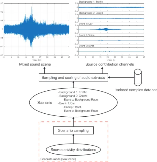
Figure 2.1 shows the sound scene construction process for the two main simulation libraries available: simScene [57] and Scaper [58]. Scaper and the replicate mode of simScene function similarly: scenes are simulated based on an input scenario describing the background and event activity of sources of interest over time. Background sources are active for the duration of the sound scene. The first background (class traffic in Figure 2.1) consti-tutes the reference in terms of sound level. Additional background sources (class crowd in Figure 2.1) are associated with an event-to-background ratio (EBR) corresponding to the emergence of the event compared to the overall background activity (expressed in dB), and from which the corresponding extracts are scaled.
Scenario sampling
Source activity distributions
Generate mode (simScene)
Isolated samples database
Scenario - Background 1: Traffic - Background 2: Crowd - Event-to-Background Ratio - Event 1: Car - Onset/Offset - Event-to-Background Ratio ...
Sampling and scaling of audio extracts
Source contribution channels Mixed sound scene
Background 1: Traffic
Background 2: Crowd
Event 1: Car
Event 2: Voice
Event 3: Birds
Figure 2.1: Overview of the scene simulation process from scenarios and a database of isolated source samples.
Event sources are defined by onset and offset timestamps, as well as an event-to-background ratio with all combined background sources as refer-ence. From the input scenario, source contributions are pseudo-randomly sampled from a database of isolated samples, which comprises extracts of isolated occurences of a specific source. The simulation process outputs con-tributions of each source as separate channels, and combines them additively to produce the sound scene. For sound event detection (SED) datasets cre-ation, Scaper additionally allows data augmentation on the isolated samples database with pitch shifting and time stretching techniques.
Figure 2.2: Map of the soundwalks and 19 recording locations in the 13th district of Paris presented in [1]. Sound levels shown on the soundwalk path are interpolated from measurements at each location.
The generate mode of simScene is oriented towards creative use cases, as it allows the generation of original scenarios. The term scenario refers to an ensemble of all properties characterizing sounds in polyphonic scenes, in-cluding the taxonomy of sources and structural parameters describing their activity [59]. Instead of scalar onset-offset and event-to-background ratio values, the simulation process in this mode is given the mean and standard deviation of a normal distribution for each source and simulation parame-ter. Original scenarios are composed by pseudo-randomly sampling these distributions. This process can be seen as performing data augmentation on a reference (average) sound scene scenario by applying random variations to its defining high-level properties, where these variations are controlled to remain plausible. Conditioning distributions on ambiances, i.e. inferring a different set of reference sound scenes as well as variation range for each cat-egory of sound environment, then results in a large dataset of sound scenes covering diverse scenarios encountered in urban environments.
The capacity of a deep learning model to generalize to possible urban sound environments depends on the quality of the training data. In other terms, the simulated scenes composing the training dataset should contain
diverse scenarios covering as many real-life situations as possible while re-maining within the scope of plausible environments. To do so, the corpus of 74 recordings proposed in [1] is taken as a reference for the parameters of the scenario generation process.
This reference corpus, on which the TFSD indicator described in Sec-tion 1.3 is developed, was gathered as part of the GRAFIC project during four soundwalks in the 13th district of Paris. Sound scenes ranging from 55 s to 4.5 min in duration were recorded at 19 locations (P1-19) with diverse en-vironments as shown in Figure 2.2. These recordings were classified in [60] as representing quiet street, noisy street, very noisy street and park ambiances.
2.2
Subjective annotations
2.2.1 Motivation
The capabilities of simScene’s generate mode are useful for creating large datasets with diverse ambiances and polyphonic levels, but raise some con-cerns about perceptual responses produced by simulated scenes. A deep learning model will be trained to predict perceptual descriptors on simu-lated scenes, then applied to real-life sensor data derived from recordings. There is thus a need to ensure that intrinsic differences between simulated and recorded scenes do not result in significant changes in terms of percep-tion, both overall and in terms of active sound sources. Such differences exist at two levels: the additive composition of simulated scenes does not fully re-flect the propagation and interactions of sound sources in real-life conditions, and the scenarios, although derived from existing environments, are original. The effect of the first factor on perception can be studied by manually an-notating reference recordings, and using the resulting scenarios to simulate sound scenes with almost identical content in terms of source activity. Dif-ferences between perceptual evaluations of paired recorded-replicated sound scenes on individual descriptors can then be investigated. Assessing the im-pact of the second factor is less straightforward, because there is no direct correspondence between real-life and generated scenarios to compare quan-titative assessments on. Evaluation should thus be conducted on a larger corpus to assess potential changes in the behavior of perceptual quantities.
Furthermore, the performance of an indicator proposed for the auto-matic annotation of perceived source presence in simulated scenes has to be evaluated with respect to subjective annotations of the time of presence. Lastly, the quality of high-level attributes estimated from predictions of a deep learning model as described in Section 1.4 should be evaluated in the