Overview on the Evolution of Near Magnetic Field Coupling Prediction Using Equivalent Multipole Spherical Harmonic Sources

HAL Id: hal-01432166

https://hal.archives-ouvertes.fr/hal-01432166

Submitted on 4 Feb 2018

HAL is a multi-disciplinary open access

archive for the deposit and dissemination of

sci-entific research documents, whether they are

pub-lished or not. The documents may come from

teaching and research institutions in France or

abroad, or from public or private research centers.

L’archive ouverte pluridisciplinaire HAL, est

destinée au dépôt et à la diffusion de documents

scientifiques de niveau recherche, publiés ou non,

émanant des établissements d’enseignement et de

recherche français ou étrangers, des laboratoires

publics ou privés.

Coupling Prediction Using Equivalent Multipole

Spherical Harmonic Sources

Arnaud Bréard, Olivier Chadebec, Laurent Krähenbühl, Carlos Sartori,

Christian Vollaire, Olivier Fabrègue, Zhao Li, Rafael P. B. Muylaert, François

Tavernier, Damien Voyer

To cite this version:

Arnaud Bréard, Olivier Chadebec, Laurent Krähenbühl, Carlos Sartori, Christian Vollaire, et al..

Overview on the Evolution of Near Magnetic Field Coupling Prediction Using Equivalent

Multi-pole Spherical Harmonic Sources. IEEE Transactions on Electromagnetic Compatibility, Institute

of Electrical and Electronics Engineers, 2017, 59 (2), pp.584-592. �10.1109/TEMC.2016.2638960�.

�hal-01432166�

Abstract — In the ElectroMagnetic Compatibility (EMC)

behaviour of power electronic converters, parasitic magnetic couplings between components are one of the main causes of dysfunctions or poor filtering. These couplings may be either conducted or near-field interferences. To handle interaction problems, full knowledge of these magnetic couplings is essential. This article is an overview of the work on near magnetic field interference undertaken in the last 15 years by the International Maxwell Laboratory. This paper details a predictive method that accurately and efficiently calculates near magnetic field coupling between two sources. The method uses near-field multipolar expansion in spherical harmonics of electromagnetic sources to determine close magnetic coupling between two sources from their equivalent models. This paper also shows how theoretical developments of large loop antennas have evolved from the van Veen antenna, a model with only two degrees of freedom, to a more complex model in terms of degrees, order and types of harmonics. In parallel, it describes developments in the measurement method that provides input to the theoretical model. To illustrate how the research has evolved, we discuss coupling between two complex sources to assess the accuracy of this predictive method.

Index Terms — Electromagnetic Compatibility, near magnetic

field coupling, power electronics, spherical harmonics.

This work was partially supported in France by ANR (ANR-10-VPTT-0013 and ANR-14-CE22-0009), in Brazil by CNPq under the PQ 307867 2011-0 grant scheme and by the Franco-Brazilian CAPES-Cofecub grant 503/05.

A. Bréard, L. Krähenbühl, C. Vollaire, O. Fabrègue, Z. Li, F. Tavernier and D. Voyer are with Université de Lyon, CNRS, Ampère (CNRS UMR5005), ECL, F-69134 Écully, France (e-mail: arnaud.breard@ec-lyon.fr).

O. Chadebec, is with Université Grenoble Alpes, CNRS, G2Elab (CNRS UMR5269), F-38000 Grenoble, France.

C. A. F. Sartori and R. P. B. Muylaert are with Escola Politécnica PEA-EPUSP, Av. Prof. Luciano Gualberto - Trav. 3, 380 - 05508-010, São Paulo, SP, Brazil. C. A. F. Sartori is also with Instituto de Pesquisas Energéticas e Nucleares IPEN/CNEN-SP. Dept. SRC. Trav. R 400 - 05508-900, São Paulo, SP, Brazil.

A. Bréard, O. Chadebec, L. Krähenbühl, C. A. F. Sartori, C. Vollaire, O. Fabrègue and D. Voyer, and are also with Laboratoire International Associé franco-brésilien James Clerk Maxwell (“LIA Maxwell” - CNRS LIA817) CNPq, UFMG, UFSC, EP-USP (Brazil) – Univ. Grenoble Alpes, Univ. de Lyon (France).

I. INTRODUCTION

evices using power electronics are becoming almost ubiquitous. However, power electronics systems are intrinsic sources of ElectroMagnetic Interference (EMI). Power density increases as the technology advances, producing more and more sources of electromagnetic disturbance. These sources degrade the performance of other electronic devices in the vicinity, and vice versa. Therefore, characterizing the EMI generated within power electronics systems and the near-field couplings between these sources of disturbance has become an important aspect in the study of EMC system behaviour, the aim being to optimize the nominal performance of any electronic device in the presence of other systems. However, EMC behaviour is quite often addressed only after the prototype has already been developed. The conventional approach is empirical and based on experimental trial and error processes that seek to ensure that the existing prototype complies with EMC standards [1]. This results in additional costs and significant manufacturing delays in the case of dysfunctions due to EMI. It is therefore increasingly important to consider EMC behaviour in the design process before physical prototyping. This is why predictive EMC modelling methods need to be developed.

The electrical signals in complex power electronic systems (converters) are high currents with rapid variations, which means that near magnetic field coupling is the main cause of dysfunctions or poor filtering. The focus here is therefore on near magnetic field coupling either between components (intra-system coupling) or between systems (inter-system coupling).

The method we have been developing for several years is based on multipole expansions in spherical harmonics of the near-field around sources. Each source is represented by an equivalent point multipole, which allows near-field couplings to be calculated efficiently [2]. During the design stage of a system, virtual knowledge of these couplings enables the relative positions of its components to be optimized to keep electromagnetic interactions to a minimum [3].

Advances using multipole models have also had an impact on the development of test benches for near-field measurements. The co-evolution of “theoretical versus test” bench approaches will be presented in Section II thorough a

Overview on the Evolution of Near Magnetic

Field Coupling Prediction using Equivalent

Multipole Spherical Harmonic Sources

A. Bréard, O. Chadebec, L. Krähenbühl,

C. A. F. Sartori, C. Vollaire

O. Fabrègue, Z. Li, R. P. B. Muylaert, F. Tavernier and D. Voyer

historical overview: the pioneering system based on the van Veen & Bergervöet antenna principle [4] using fixed coils and developed since the early 2000s [6][34]; the concept of “spatial filtering” and related ideas on building workable test benches and then simplifying the arrangement of coils when identification of a higher degree and order is needed. The link between near field and mutual inductance assessments will also be discussed [5].

In section III, current developments with our two measu-rement test benches (one in São Paulo, Brazil, the other in Lyon, France) will be described, with some examples of results.

II. HISTORICAL OVERVIEW OF THE RESEARCH

A. The van Veen & Bergervöet antenna prototype

The van Veen and Bergervöet antenna consists of orthogonal arrangements of three loaded loop antennas [4]. The antenna loops are constructed with coaxial cable, and their load impedances, which are located at opposite sides of the loops, consist of two impedances connected to the inner and outer conductors of the coaxial cable. In a typical measurement setting, the Device Under Test (DUT) is located in the centre of the loops, so that the emissions radiated from the DUT induce currents through it by electromagnetic coupling. These currents are measured, and the radiated fields can then be calculated and characterized. The aforementioned pioneering studies on the use of loop antennas to obtain equivalent sources started with the development of a van Veen & Bergervöet antenna prototype as a student project in 1997, on which a paper was presented in 2000 [34]. Initially, this covered the main aspects concerning details of the design and construction of an antenna prototype, and its calibration in accordance with CISPR 15 [17]. An investigative study on the influence of the electromagnetic environment was carried out in the 9kHz-30MHz frequency range. The influence of distance from walls, metallic conductors, etc. in different sites was also investigated [6]. The radiated emissions of a number of lighting system samples were assessed as an application. The simplicity of this antenna setup, its low cost and the accuracy of the results obtained in these studies drew the attention of the authors to the idea of using the loop antenna configuration as a method for determining equivalent radiated emission source models in NF, suitable for NF-FF evaluation. Thus, magnetic dipoles could be calculated and used as equivalent radiated sources in previous studies [6]. Other similar loop antennas can be used for this purpose, like the one proposed by Kanda and also studied by the authors of papers [35][36]. When comparing these antennae, different frequency responses can be realized. In particular, the van Veen and Bergervöet antenna produces a flatter response at low frequencies, up to MHz, to variations in load and geometrical parameters [36]. The need to represent the radiated sources with a higher order of precision has led us to propose new arrangements or configurations of loop sensors and the use of multipolar expansion in spherical harmonics. These are discussed in the following sections.

B. Multipolar expansion in spherical harmonics

J. Lorange [10] shows that the near field may be obtained using real, scalar spherical harmonics. In this study, the frequency range is 20kHz-30MHz and distances are less than one metre, so that a quasi-static approximation is appropriate:

0

∇× Β ≈ (1)

outside a simply-connected volume containing the electrical currents (i.e. the source to be characterized). Thus, the magnetic field is (outside this volume)defined by the gradient of the magnetic scalar potential ψ :

0 µ ψ

Β = − ∇ . (2)

B being conservative (∇. 𝐵 = 0), ψ is solution of the Laplace equation:

∇2_{𝜓 = 0. (3)}

In spherical coordinates (with the “expansion centre” r=0 in the volume containing the source) the potential 𝜓(𝑟, 𝜃, 𝜑) can be developed in spherical harmonics as follows [8][9][27]:

(

)

(

)

ψ

θ ϕ

θ ϕ

∑ ∑

Qnm are the unknown coefficients to be determined. For a

given source, these depend on the particular choice of the spherical system (expansion centre, direction).

Ynm(𝜃, 𝜑) are the spherical harmonic functions of degree n and

order m (Fig. 1), expressed in terms of Legendre polynomials for 𝜃 and m-periodic functions for 𝜑 [11]. These Ynm functions

are orthogonal:

∫ 𝑌_𝑖𝑖(𝜃, 𝜑). 𝑌_𝑛𝑛(𝜃, 𝜑)𝑑𝜃𝑑𝜑 = 0 𝑖𝑖 (𝑖, 𝑗) ≠ (𝑛, 𝑚). (5)

Figure 1: Spherical harmonic functions Ynm(θ,ϕ) for n up to 4 and m ≥ 0 [19]. The near magnetic field can then also be written as a multi-polar expansion, using the same coefficients Qnm:

(

)

(

)

(

)

θ ϕ

µ ψ

θ ϕ

θ ϕ

∑ ∑

with:

(

)

µ

_{θ ϕ}

π

Because of Eq. (1), developments (4) and (7) are only valid for r>r0, where r0 defines the smallest sphere that contains all the electrical currents (“sphere of validity”.)

C. Mutual Inductance calculation with spherical expansion The final goal is the assessment of inductive coupling between components or systems. In network analysis, this coupling corresponds to mutual inductances. The link between magnetic near-field and mutual inductance was brought to light by Rumsey [12] and Richmond [13]. The report by B. C. Brock on the translation of the expansion centre of spherical harmonics [5] (also partially based on [14]) then provided a practical way of computing the mutual inductance between two systems produced by the development of their spherical harmonics. In addition, the rotations of each system influence coupling and also have to be considered [15].

For quasi-static studies, the near magnetic field of system i can be represented as a function of iQn,m; the mutual

inductance M12 between systems i and j can be determined by [17]:

𝑀12 ~ ∑𝑛=1∞ ∑𝑛𝑛=−𝑛(−1)𝑛�1𝑄𝑛,−𝑚_𝐼1 .2𝑄_𝐼2𝑛,𝑚�. (8) The accuracy of the mutual inductance computation increases with the maximum degree of expansion used to represent the sources i and j. The complexity (number of coefficients) grows in (2n+1) with degree n of the model.

For experimental verification, the mutual inductance between coils can be determined with a Vector Network Analyzer (VNA), using the current ratio (I2/I1) and direct

measurement of the self-inductances:

𝑀21= 𝐿2.𝐼_𝐼2₁= 𝐿1.𝐼_𝐼1₂. (9) D. Spatial filtering

In [18], Kildishev et al. present spatial filtering measurements to estimate the dipolar and quadrupolar components of the magnetic field of a spacecraft. The main idea of spatial filtering is as follows: for a given distance r (on the surface S of a sphere), the normal induction (Eq. 2 and 4) is given by:

𝐵�⃗._𝑟𝑟⃗= − ∑𝑛=1+∞ (𝑛+1)_𝑟𝑛+2 ∑𝑛=−𝑛𝑛=𝑛 𝑄𝑛𝑛. 𝑌𝑛𝑛(𝜃, 𝜑). (10) Now consider the following quantity 𝜉_𝑖𝑖 defined on S:

𝜉𝑖𝑖(𝜃, 𝜑, 𝐵𝑛) = 𝑌𝑖𝑖(𝜃, 𝜑). 𝐵𝑛 (11) which is the normal flux density, weighted by the spherical harmonic function of degree i and order j. As Ynm are

orthogonal functions (Eq. 5), the flux of 𝜉_𝑖𝑖 through the surface S depends on just one coefficient, 𝑄_𝑖𝑖 (the term in brackets does not depend on B):

� 𝑌𝑖𝑖(𝜃, 𝜑). 𝐵𝑛 𝑆 . 𝑑𝑑 = � 𝜉𝑖𝑖(𝜃, 𝜑, 𝐵𝑛) 𝑆 . 𝑑𝑑 = −𝑄𝑖𝑖. �(𝑖+1)_𝑟𝑖+2∬ 𝑌𝑆 𝑖𝑖2(𝜃, 𝜑)𝑑𝑑�. (12) This means that this flux produces a direct and exact measurement of the coefficient Qij. This defines the ideal

weighting, which can be used in numericalsimulations but is not experimentally feasible. The challenge of spatial filtering is to obtain the best experimental approximation of this ideal case, by using linear combinations of flux measurements in judicious arrangements of simple coils, i.e. to approximate the smooth function 𝑌_𝑖𝑖(𝜃, 𝜑) on the sphere with the simplest possible constant piecewise function (an example will be given below, Fig. 4). These linear combinations may be made directly by connecting a set of real coils or a posteriori by post-processing when there are no simultaneous measurements (for example using one moving coil).

1) First approach: degrees n≤2 (zero order m=0)

B. Vincent et al. [19][20], then S. Zangui et al. [21][22], pro-posed a method to identify exactly the 8 dipolar and quadrupolar coefficients (3 coefficients for n=1 and 5 for n=2), on the assumption that the harmonic expansion of the near magnetic field is limited to the 4 first degrees (n=1 to n=4): if the real field contains any higher-degree components (n≥5), the identification of these 8 low-degree coefficients will no longer be exact.

We will now consider the behaviour of the spherical harmonics (Fig. 1) and their symmetries, first for m=0 (the field does not depend on ϕ). Fig. 3 shows the corresponding spherical coaxial test bench. The central coil is on the plane of the source: it will give a zero response for both non-symmetrical functions Y10 and Y30 and no response for the

symmetrical functions Y20 and Y40.

Figure 2: Measurement prototype developed in [8] to identify the dipolar and quadrupolar coefficients of expansion (order m=0).

By replacing this coil with system C10 comprising two

symmetrical coils connected in series (and coiling in the same direction), it becomes possible to cancel the contribution of Y30

(by adjusting the distance between the two coils). Similarly, the two symmetrical coils of system C20 are connected in

series (but coiling in the opposite direction), which gives a zero response for the non-symmetrical functions Y10 and Y30.

The effect of Y40 can be cancelled by adjusting the distance.

In this way the pair of coils C10 measures Y10 with no

influence of Y30 (Y20 and Y40 have no effect because of their

symmetry). The pair C20 (coiling in opposite directions) gives

a signal for Y20 with no influence of Y40 (Y10 and Y30 have no

effect because of their anti-symmetry).

The distances between coils in C10 and C20 are defined by

the cancellation of the Y30 and Y40 fluxes, respectively giving

θ1=63.5° for C10 and θ2=41° for C20 (Fig. 2).

The computation of near-field coupling by using these multipolar coefficients was then validated by comparison with the numerical results from the Flux3D© software [28] for a simple case between two 1-turn-coils and measurements with a van Veen and Bergervöet antenna [8].

2) Degrees n≤2, non-zero orders (m=1 or m=2).

a) Adapted coil for spatial filtering

By applying the principle of spatial filtering described above, it is also possible to address non-zero orders. In 2009, B. Vincent et al. showed how to build this kind of complex coil systematically [19]. We give an example below for the function Y22: this function (Fig. 1) produces 4 flux lobes

around the vertical axis, alternately positive and negative. Using 4 coils (with a 90° angular width) connected in such a way that the 4 fluxes are additional (Fig. 3 a) will capture the maximum possible value of the flux. Because of the symmetries, this configuration cancels the flux of all Ynm, n≤4,

except for Y42, although the latter flux may be cancelled out by

a symmetrical reduction of the height of the 4 coils (Fig. 3 b) to give a vertical angular width of 91.54°. Fig. 3 (c) shows the values of the resulting constant piecewise weight function and its high correlation with Y22.

(a) (b) (c)

Figure 3: Steps to define the Y22 sensor: (a) configuration giving the maximum

possible flux; (b) modification in order to cancel the effect of Y42;

(c) corresponding values of the final constant piecewise weight function.

b) Spatial filtering using moving circular coils

Obviously, the kind of sensor described above is non planar and will be difficult to build. This is why (just some months later) we proposed [20] to apply spatial filtering using only simple circular coils attached to the sphere (Fig. 2), or one coil moving around the sphere: the coil positions are then defined by (𝜃, 𝜑) rotations. The basic idea comes from the following observation: Y1,-1 and Y11, are identical to Y10 except for one

rotation (Fig. 1); similarly, it is possible to reconstruct Y22

using only Y20 and two different rotations (Fig. 4):

√3𝑌22 = − 𝑌20 𝜋 2;𝜋2_{+ 𝑌} 20 𝜋 2;0_{. (13)}

Sensor C10 in Fig. 2, which was designed for direct

measurement of Y10, may then be used (after appropriate

rotation) for Y1,-1 and for Y11; sensor C20 was designed for Y20

and may be reused for Y22 and Y2,-2 by combining (post

processing) the two measurements obtained for the two adapted rotations. It is easy to generalize this principle: the device in Fig. 2 associated with a system of 2-axis rotations allows the 3 dipolar and 5 quadrupolar coefficients of multipolar expansion of the source to be identified.

Figure 4: Construction of Y22 from rotations of Y20. 3) Extension to higher degrees (n≤ 4).

The analysis of the mutual inductance estimation from developments of degree 2 shows that in some cases, the dipolar and quadrupolar degrees are not sufficient: the relative error for M21 may be higher than 50% because the distance

between the two components being tested is shorter than twice the size of the DUTs [2]. In order to improve accuracy, Hoang et al. [17] extended the previous study to degrees 3 and 4,on the assumption that degrees n≥7 are negligible. The design of the C30 and C40 coils follows the same principle as for C10 and

C20 (§II-D.1), giving 2 solutions for each degree: θ3,1=40.09°

or θ3,2=73.43° for C30 and θ4,1=33.88° or θ4,1=62.04°for C40

(Fig. 5).

Figure 5: Completed measurement prototype with twelve coil sensors for identification of the multipolar expansion (n ≤ 4) [17].

In the same study, this 12-coil test bench was used to test the accuracy of the mutual inductance estimation between a dipole and a quadrupole, and between a dipole and an octupole according to the maximum degree (2 or 4)of expansion. Some

complex sources, such as transformers and toroidal inductors, were also characterized up to degree n=4. In this case, n(n+2) = 24 components have to be identified, using 120 flux measu-rements and 25 different orientations of the test bench.

Therefore, this method cannot be implemented efficiently without advanced automation of the entire process.

III. AN AUTOMATIC NEAR-FIELD MEASUREMENT SYSTEM

A. Spheroidal automated system developed at LMAG (SP) In the previous section, we discussed developments in radiated near-field measuring systems and their importance, including the near-field loop antenna systems developed by the authors. One of the characteristics to be mentioned is the need to reposition either the device under test (DUT) or the sensors, for each of the measurements. Although this is time-consuming, it is necessary to ensure that the components accurately characterize the radiated sources.

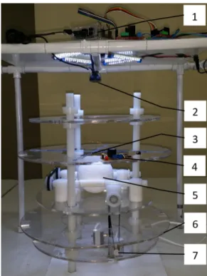
In order to minimize the aforementioned constraints, a prototype of an automated measurement antenna system was built and calibrated for the 9kHz-30Mhz frequency band. Basically, the system consists of a set of loop antennas, placed in fixed positions around a moving sphere that is used to house the DUT. The whole can be moved with 3 degrees of freedom: Stepper motors connected to a pulley and clutch system are available for this purpose, while cameras provide machine vision feedback which is applied to achieve the desired precision in positioning (Fig. 6).

Figure 6: Details of the automated measurement system: 1) Raspberry Pi; 2) Visual Feedback camera; 3) Fixed markers; 4) Current Probe; 5) Sphere containing the DUT; 6) Loop sensor; 7) Stepper motors

Although spherical harmonics have been used up to now in the electromagnetic algorithm, the proposed system is also suitable for implementing the equivalent cylindrical

harmonics [11][17]. Higher levels of precision can thus be achieved once higher orders and degrees or components of multipolar expansion can be obtained with the system. Figure 1 presents details of the automated near-field measurement prototype, which is suitable for evaluations of components up to n=4 (dipoles and quadrupoles).

1) Automation and Measurement Process

All the movement control, image gathering and data processing functions are provided by a widely available raspberry pi computer system programmed with Python and related Simple CV libraries, which include colorDistance, Binarize and Findlines [29]. The automation system accepts a list of pre-assigned relative DUT and loop sensor positions which, when they are set accordingly, enable the parts of the system to reach the desired positions.

When positioning is complete, the data acquisition system is activated and begins the measurement and post-processing cycles. To avoid contributions from the inner equipment and accessories, such as motors, these are configured to be shut down while the measurements are being made. Furthermore, the system layout was carefully designed on the basis of the experimental approach to minimize field couplings to the loops.

2) System robustness and positioning precision

Due to the positioning method adopted, the maximum positio-ning precision of the system depends only on the resolution of the camera and on its distance from the radiated source. An iterative process is applied while the measuring and repositioning steps are carried out, until the desired position is reached [30].

If a failure should occur during this process, the system will randomly reposition the DUT and restart the iteration process, allowing it to run without continuous oversight. Moreover, the maximum positioning error may be set by the user to shorten the repositioning cycles.

For the current system prototype, a camera with 640x480px resolution is used, resulting in 0.35mm/px accuracy on the top of the surface of the sphere, which corresponds to a 1º arc for a maximum error of 1 px in the 12cm sphere.

This bench is currently being developed at LMAG, Escola Politécnica of Sao Paulo (Brazil).

B. Single coil automatic test bench developed in Lyon 1) Description and optimization

Another automatic test bench for near-field measurements is currently being developed and tested at the Ampère Lab in Lyon (France). This test bench (Fig. 7) comprises a rotating support (angle φ) for the DUT and a rotating arm (angle θ) holding a single sensor coil. Rotation is activated by a remote motor. The DUT and the sensor coil are connected to a Vector Network Analyser (VNA) via BNC connectors. The motors and the VNA are controlled by a JAVA program. The VNA provides measurements of the voltage (direct) or current

(using current probes) ratios between source and sensor. Due to the limitations of the current probe, the dynamic is 10 to 30 times better for voltage measurements.

When using this test bench, we abandoned the idea of direct coefficient extraction by spatial filtering. The principle will now be to accumulate a large number of measurements m and to identify the source of degree n using post-processing tools, including the least square method to reduce the full m x n matrix to a square system with only n(n+2) unknowns.

Figure 7: Automated test bench including (θ,ϕ ) rotations. 8<a<30cm; 10<b<30cm -5<h<5cm; -120<θ<120°; 0<ϕ <360°]

The size of the coil sensor is selected to optimize identification while taking uncertainties in the bench parameters into account: sensor position (±0.1°), source position (±1mm), source orientation (±0.5°), arm length (±1mm) and noise (1E-10Wb). This optimization is based on the Bayesian approach and the MIPSE software developed in Grenoble [31]. This software includes the GOT-it optimization algorithms [32] and the propagation of uncertainties [33].

Finally, a radius of 6 cm for the coil sensor proved to be the best compromise for an expansion of degree 4 and measurements on a sphere of radius 20 cm (Fig. 8).

Figure 8: Normalized uncertainties according to sensor radius for a distance of 20cm.

2) Preliminary results

With this new test bench, initial results were obtained for the coupling between two printed circular coils with radii of 5cm

and 3 cm respectively. The near-field of each dipole was characterized by uniformly distributed measurements in the range of -120<θ<120° using a coil sensor of radius 5 cm at a distance of 10 cm from the DUT. To reduce noise, the measurements were made at an intermediate frequency (IF) filter bandwidth of 3Hz, taking an average every 10 runs. This took 20 minutes for 5 frequencies. A least square method was then applied to build the equivalent models, the first incorporating only dipolar and quadrupolar components and the second incorporating the first four degrees. For these z-oriented dipoles, it should be noted that only zero-order functions are likely to contribute to expansion.

The results for these two coils are summarized in Table I.

TABLE I

COEFFICIENTS FOR 2 CIRCULAR COILS:

COMPARISON OF THE REFERENCE ANALYTICAL SOLUTION [37]

WITH THE RESULTS OF DEGREE 2 AND DEGREE 4 IDENTIFICATIONS. Radius Model Q10 Q20 Q30 Q40

5 cm analytic 7.85E-3 0 -1.47E-5 0 2 coeff. 8.54E-3 -1.13E-4

4 coeff. 7.99E-3 -3.80E-5 -1.93E-5 -2.61E-7 3 cm analytic 2.82E-3 0 -1.91E-6 0

2 coeff. 3.03E-3 -2.06E-5

4 coeff. 2.95E-3 4.86E-6 -3.05E-6 -2.62E-8

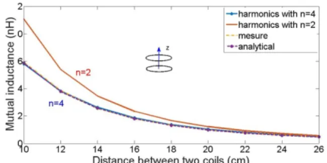
Based on these coefficients and Eq. 8, the mutual induc-tance can be computed according to the disinduc-tance (z direction) between the two coils and compared with the measurements made (Fig. 9). The relative error (Fig. 10) between the measurements and the analytical model is lower than 1%.

Figure 9: Mutual inductance between 2 coaxial horizontal coils according to the distance following the z axis, at a frequency of 300 kHz.

Figure 10: Relative error in the mutual inductance estimation according to the distance, along the z axis, between measurements and spherical harmonics with n=2 and n=4, at a frequency of 300 kHz.

When the distance between the coils is short, the results for identification of degree 2 are poor (50% relative error for

10cm). In contrast, the maximum relative error for degree 4is 5%, which is lower than our previous results [2][17].

IV. CONCLUSION

Since 2004, part of the research by LIA Maxwell has focused on modelling near-field couplings of electronic devices. This study on near-field measurements started with the van Veen Antenna and moved on to spatial filtering. The model deve-loped was based on spherical harmonics with multipolar expansion, from two degrees at the start, expanding to four degrees and then generalized to N degrees. With the addition of the Bayesian approach, the latest measurement test bench proved to be more accurate than the previous versions. The automation of the measurements and the most recent approach (described in part III.B) reduces the time needed to characterize the near field emitted by a DUT by a factor of 16 for modelling up to the fourth degree. The initial results show a high level of agreement between the measurements and the analytical model and also for the spherical model with a minimum of four degrees.

In future studies, both test benches will be used to characterize more complex sources and to compare their performance in terms of precision and the time required for full characterization. They will be also used for further developments on different types of harmonics. The authors are applying and suggesting the use of the proposed sensor arrangement to characterization and control the on-board system radiated emission, and as a non-invasive failure detection approach, based on the resulting magnetic signature assessment.

REFERENCES

[1] E. Hoene, “EMC in Power Electronics,” in Proc. 5th Int. Conf. on

Integrated Power Systems (CIPS ’08), pp. 1–5, March 2008.

[2] S. Zangui, “Détermination et Modélisation du Couplage en Champ Proche Magnétique entre Systèmes Complexes,” PhD dissertation n° 2011-ECDL-0029, tel-00681821, Ecole Centrale de Lyon, 2011. [3] P. Fernandez-Lopez, T. D. Pham, T. Q. V. Hoang and F. Lafon, “A

methodology to design an EMC filter layout providing optimal response based on simulation and considering the inter-component couplings,”

18th Int. Symposium on EMC, Rennes, France, July 2016.

[4] J. R. Bergervoet and H. Van Veen, “A large-loop antenna for magnetic field measurements,” in Proc. of Zurich International Symposium on

EMC, 1989, pp 29-34.

[5] B. C. Brock, “Using vector spherical harmonics to compute antenna mutual impedance from measured or computed fields,” SANDIA Report,

SAND2000-2217-Revised, Sandia National Laboratories, 2001.

[6] M. Savi, T. Z. Gireli, F.A. Tirich and C. A. F. Sartori, “Developing a Van Veen & Bergervoet Antenna,” in Proc. of EMC 2004, pp. 717-720. [7] Standard CISPR 16-1, part P, 2002, pp. 230-237 and 396-409.

[8] B. Vincent, “Identification de sources électromagnétique multipolaires equivalents par filtrage spatial : Application à la CEM rayonnée pour les convertisseurs d’électronique de puissance,” PhD dissertation, tel-00473780, Grenoble INP, 2009.

[9] C. J. Bouwcamp and H. B. G. Casimir, “On multipole expansion in the theory of electromagnetic radiations,” Physica, Vol. 20, Issues 1-6, 1954, pp. 539-554.

[10] J. Lorange, “Couplage des inductances par rayonnement magnétique. Etude théorique et expérimentale,” PhD dissertation, tel-00599643, Grenoble INP, 2001.

[11] J-C. Nédélec, “Acoustic and Electromagnetic Equations – Integral Representations for Harmonic Problems,” Springer, 318 pages, 2001.

[12] V. H. Rumsey, “Reaction Concept in Electromagnetic Theory,” Physical

Review, vol. 94, no. 6, pp 1483-1491, June 15, 1954.

[13] J. H. Richmond, “A Reaction Theorem and Its Application to Antenna Impedance Calculations,” IRE Transactions on Antennas and

Propagation, Vol. AP-9, no. 6, pp. 515-520, November 1961.

[14] A. Messiah, “Clebsch-Gordan (C.-G.) Coefficients and “3j” Symbols,”

in Appendix C.I in Quantum Mechanics, vol. 2, pp. 1054–1060,

North-Holland, Amsterdam, The Netherlands, 1962.

[15] R. Green, “Spherical harmonic lighting: The gritty details,” in Proc.

Game Dev. Conf., pp. 1–47, 2003.

[16] M. A. Blancoa, M. Floreza, and M. Bermejo, “Evaluation of the rotation

matrices in the basis of real spherical harmonics,” Journal of Molecular Structure (Theochem), pp. 19-27, 1997.

[17] T. Q. V. Hoang, A. Bréard, and C. Vollaire, “Near Magnetic Field Coupling Prediction Using Equivalent Spherical Harmonic Sources,”

IEEE Trans. on EMC, Vol. 56, n°6, pp. 1457-1465, 2014.

[18] A. V. Kildishev, S. A. Volokhov and J. D. Saltykov, "Measurement of the Spacecraft Main Magnetic Parameters," IEEE Autotestcon

Proceedings, pp. 669-675, 1997.

[19] B. Vincent, O. Chadebec, J.-L. Schanen, C. A. F. Sartori, L. Krähenbühl, R. Perrussel, and K. Berger, “New robust coil sensors for near field characterization,” J. Microw. Optoelectron. Electromagn. Appl., vol. 8, no. 1, pp. 64S–77S, 2009.

[20] B. Vincent, O. Chadebec, J. L. Schanen, K. Berger, R. Perrussel and L. Krähenbühl, “Identification of Equivalent Multipolar Electromagnetic Sources by Spatial Filtering,” IEEE Trans. on Mag, vol. 46, no. 8, pp. 2815–2818, 2010.

[21] S. Zangui, K. Berger, C. Vollaire, E. Clavel, R. Perrussel, and B. Vincent, “Modeling the near-field coupling of EMC filter components,” in Proc. IEEE International Symposium on Electromagnetic

Compati-bility, pp. 825–830, 2010.

[22] S. Zangui, B. Vincent, K. Berger, E. Clavel, R. Perrussel, and C. Vollaire, “Equivalent Source Corresponding to Radiated Field of EMC Filter Components,” EMC Europe, Wroclaw, Poland, 2010.

[23] T. Q. V. Hoang, A. Bréard, C. Vollaire, L. Krähenbühl, C. Sartori. “Complete Identification for Near-Field Multipolar Expansion of Electromagnetic Sources,” CEFC, Annecy, France, 2014.

[24] L.-L. Rouve, L. Schmerber, O. Chadebec, and A. Foggia, “Optimal Magnetic Sensor Location for Spherical Harmonic Identification Applied to Radiated Electrical Devices,” IEEE Trans. on Mag., vol. 42, n° 4, 2006.

[25] E. B. Saff and A. B. J. Kuijlaars, “Distributing many points on a sphere,” Math. Intelligencer 19 (1), 5–11, 1997.

[26] C. A. F. Sartori, S. Zangui, M. Ferber, B. Vincent, R. Perrussel, C. Vollaire, L. Krähenbühl, “Calibration methods for a large loop antenna measurement system,” in Proc. of Compumag, Sydney, Australia, 2011. [27] J. P. Wikswo, “Scalar multipole expansions and their dipole

equiva-lents,” J. Appl. Phys. 57 pp. 4301-4308, 1995. [28] http://www.cedrat.com/en/software/flux.html

[29] K. Demaagd, et al. “Practical Computer Vision with SimpleCV: The Simple Way to Make Technology See,” O'Reilly Media, Inc., 2012. [30] W. S. Levine, “The control handbook (first ed.),” CRC press, 1996. [31] O. Pinaud, O. Chadebec, L.-L. Rouve, J.-L. Coulomb, J.-M. Guichon

and A. Vassilev, “A Bayesian Approach for Spherical Harmonic Expansion Identification: Application to Magnetostatic Field Created by a Power Circuitry,” IEEE Trans. on EMC, vol. 57, no. 6, pp. 1501-1509, 2015.

[32] http://www.cedrat.com/software/got-it.html

[33] M. Ferber, C. Vollaire, L. Krähenbühl, “Conducted EMI of DC-DC converters with parametric uncertainties,” IEEE Trans. on EMC, vol. 55, no. 4, pp. 699-706, Aug. 2013.

[34] C. A. F. Sartori, T. Yokoji, “Desenvolvimento de um Protótipo da Antena de Van Veen & Bergervoet,” Anais do IV Congresso Brasileiro

de Eletromagnetismo, Vol. I. p. 367-370, 2000.

[35] M. Kanda and D. A. Hill, “A three-loop method for determining the radiation characteristics of an electrically small source,” IEEE Trans.

Electromagn. Compat., vol. 34, no. 1, pp. 1-3, Feb. 1992.

[36] M. H. Seko, D. V. F. Cardia, C. A. F. Sartori and S. E. Barbin. “Analysis on the Performance of Large Loop Antennas for Equivalent Radiation Sources Determination,”CEFC, Annecy, France, 2014.