Cooling and Internal Waves on the Continental Shelf
byJames Maxwell Pringle
B.A. Dartmouth College,(1990)
Submitted in partial fulfillment requirements for the degree
of the of Doctor of Philosophy
at the
MASSACHUSETTS INSTITUTE OF TECHNOLOGY
and the
WOODS HOLE OCEANOGRAPHIC INSTITUTION
June 1998
@ James Maxwell Pringle 1998
The author hereby grants to MIT and to distribute copies of this
Signature of Author...
and to WHOI permission to reproduce thesis document in whole or in part.
JointrProgram in Physical Oceanography Massachusetts Institute of Technology Woods Hole Oceanographic Institution May 1, 1998 C ertified by ... ... Kenneth H. Brink Senior Scientist Thesis Superviror A ccepted by ...
Lot"
S r.7 C' iu LF
A 7-r i LIBRARIES W. Brechner Owens Chairman, Joint Committee for Physical Oceanography Massachusetts Institute of Technology Woods Hole Oceanographic InstitutionCooling and Internal waves on the Continental Shelf
byJames Maxwell Pringle
Submitted in partial fulfillment of the requirements for the degree of Doctor of Philosophy at the Massachusetts Institute of Technology and the Woods Hole
Oceanographic Institution April 29, 1998
Abstract
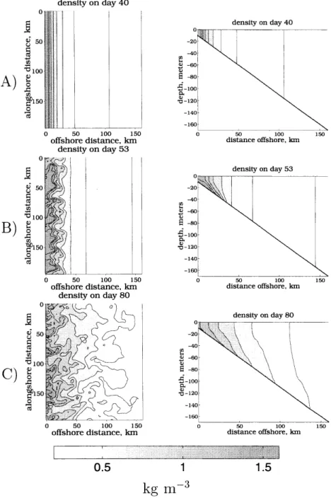
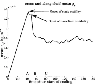
In order to begin to understand the behavior of an ice-free coastal ocean exposed to winter time cooling, the evolution of an initially homogeneous body of water undergoing uniform surface heat loss and wind forcing is examined. The dynamics of this model ocean are modulated by the intense vertical mixing driven by the surface cooling, which in the initially homogeneous ocean is sufficient to mix the entire water column in less than an inertial period. This strong vertical mixing prevents the formation of geostrophic flows and so flows are nearly down pressure gradient and downwind. Cross-shelf temperature gradients are formed by uniform cooling over water of differing depths, and these temperature gradients lead to cross-shelf density gradients. The cross-cross-shelf density gradients and flows can prevent the
cooling-driven vertical mixing from reaching the bottom when the cross-shelf bottom velocity exceeds
(where h is the water depth,
Q
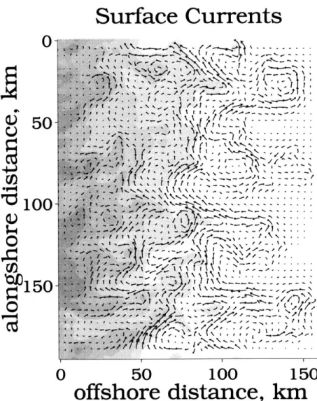
is the surface density flux representing cooling, and Op/Dy is the cross-shelf density gradient).Once the surface cooling is prevented from mixing the entire water column, alongshore geostrophic flows form, and these flows can be baroclinically unstable. The unstable flow quickly can achieve a steady state in which the length scale of the eddies is governed by either the Rhines arrest scale or a frictional arrest scale, and the surface heat flux is balanced by a cross-shelf heat flux driven by the eddies. Scales are found for the cross-shelf density gradient which results from this balance, and these scales are tested successfully in a numerical model. It is found with the numerical model that the balance between surface cooling and the cross-shelf heat flux can be attained in less than a winter with conditions typical of the Mid-Atlantic Bight.
Linear internal waves shoal and are dissipated as they cross the continental shelf, and, in order to understand how this affects the internal wave climate on the shelf, internal wave solutions are found for a wedge-shaped bathymetry. These
solutions for linear internal waves in the presence of linear bottom friction and barotropic alongshore mean flows are approximate; they are based on flat-bottom vertical modes, and the horizontal propagation is found by ray-tracing. It is found that bottom friction is capable of entirely dissipating the waves before they reach the coast, that waves traveling obliquely offshore are reflected back to the coast from an offshore caustic, and that without a mean current, the maximum distance an internal wave ray can travel along the coast is twice the distance from the shore to the offshore caustic.
The solutions for internal waves propagating over a wedge-shaped bathymetry are used to predict the evolution of an ensemble of internal waves whose properties match those of a Garrett and Munk internal wave spectrum at a point offshore. This is meant to be a simple model of the evolution of an oceanic internal wave spectrum across a continental shelf. The shape of the current ellipse caused by this ensemble of internal waves at a given frequency is found to be largely independent of frequency. It is also found that the orientation of the current ellipse is controlled by the alongshore mean currents and the "redness" of the oceanic internal wave spectrum. Because of friction, it is found that internal waves generated in the deep ocean are more likely to be important to the internal wave climate of narrow shelves than wide shelves.
The internal wave climate near two moorings of the Coastal Ocean Dynamics Experiment observation program is analyzed. It is found that the high frequency internal wave energy levels are elevated above the Garrett and Munk spectrum, and the spectrum becomes less red as one moves towards shore. The shape of the current ellipses is largely independent of frequency in the internal wave band, and the major axis is approximately perpendicular to the isobaths. The wave field is dominated by vertical-mode one waves. It is concluded that the internal wave energy is predominantly moving towards the shore from the shelf break, but that a significant portion of the internal wave energy over the continental shelf is generated over the continental shelf.
Thesis Supervisor: Kenneth H. Brink
Senior Scientist, Department of Physical Oceanography Woods Hole Oceanographic Institution
Acknowledgments
First and foremost, I would like to thank Mom, Dad, and Annie, for setting me down this path, and Ken Brink for giving me the advice I needed to stay on it until I had this thesis.
My friends kept me sane. The Dartmouth crowd, all the Jens, all the friends in the Joint Program, they all did their part. Perhaps I would have graduated more quickly without their steady distractions, but it would not have been a life I could have lived. (I would not have played as much tennis, met with a bear in a half-frozen New Hampshire swamp, gone camping in -25'F weather (Amara!), drunk vodka in Nizhny Novgorod (or fixed Russian showers in Moscow), snowboarded, grilled nearly as much, or played the part of an Austrian Duke on a train traveling incognito while suspected of a contrived plot (thanks Casa del Angst)).
My class in physical oceanography: Jay, Lyn, Bill, Natalia, Frangois, Derek, Ste-fan, Brian, & Miles, from whom I learned much of what I know about oceanography and fellowship under stress.
My officemates and housemates, Clayton, Ed, Jay, Susan, Kelsey, Alison, Gwyneth, Jim, Sarah & Steve; they seem to have survived intact.
And, of course, my committee who, with great fortitude, read way to many drafts and still gave me good comments. Without Paola Rizzoli, Steve Lentz, John Trowbridge, Glen Gawarkiewicz, and Bob Beardsley, my thesis would have been much worse.
This work was funded by an Office of Naval Research fellowship and and Office of Naval Research AASERT fellowship, N00014-95-1-0746.
Contents
1 Introduction
1.1 Winter Time Cooling and the Coastal Ocean . . . . 1.2 Observations and Theory of High Frequency Internal Waves over the
Continental Shelf . . . ... 1.3 Bibliography... . . . . 2 The Effect of Surface Cooling-Driven Vertical Mixing on Larger
Scale Coastal Dynamics, and Vice Versa.
2.1 Introduction . . . . 2.2 The Parameterization of Convection... . . . . . . . ... 2.3 Flow Fields When Convection Reaches the Bottom .. . . . . 2.4 When Does Convection Not Mix the Entire Water Column? . . . . . 2.5
2.6 2.7 2.8 2.9
When Convection no Longer Mixes to the Bottom W hen Cooling Falters . . . . Conclusions . . . . Appendix . . . . Bibliography . . . . 3 The Role of Cross-Shelf Eddy Transport in the
sponse of a Wind-Free Coastal Ocean to Winter 3.1 Introduction . . . . 3.2 Demonstration... . . . . . . . . .. 3.3 Outline of the Scaling for the Steady State &7/ay 3.4 Buoyancy/Heat Balance.. . . . . . . . .. 3.5 Scaling -p/&y from F . . . .
3.5.1 The Velocity Scale V* . . . . 3.5.2 The Correlation Between v and p: -y . . . 3.5.3 The Cross-Shelf Length Scale: L* . . . . . 3.5.4 Given V* and L*, what are F, py and C? . 3.6 Testing the Scales in a Numerical Model . . . . . 3.6.1 Flat Bottom Results . . . . 3.6.2 The Transition Between C < 1 to L > 1
Steady State Re-Time Cooling . . . . .. .. .. ... . . . . . . . . . . . . . . . . . . . . . . .. .. .. ... . . . . . . . . . . . . . . . .
3.6.3 Testing the Length and Velocity Scales . . . . 3.6.4 Where the Scaling Breaks Down . . . . 3.7 Can the Scalings Above be Used to Understand The Transient Be-havior of the Density Field? . . . . 3.8 Extending the Scalings to Passive Tracers . . . . 3.9 How do the Cross-Shelf Eddy Heat Fluxes Compare With The Wind Driven Heat Fluxes? . . . . 3.10 C onclusion . . . . 3.11 A ppendix . . . . 3.12 B ibliography . . . . 4 High Frequency Linear Internal Waves on a Sloping Shelf
4.1 Introduction . . . . 4.2 Plain Internal Wave Solution . . . . 4.3 The Path of a Wave with No Mean Flow . . . . 4.4 Wave Amplitude: the Inviscid Problem. . . . . . . .. 4.5 Wave Amplitude: the Frictional Problem . . . . 4.6 Internal Waves in the Presence of a Barotropic Mean Flow . . . . . 4.7 Current Meter Observations- The No Mean Flow Case . . . . 4.8 Current Meter Observations- The Mean Flow Case . . . . 4.9 C onclusions . . . . 4.10 Appendix A: The Internal Wave Bottom Boundary Condition . . . 4.11 Appendix B: The Caustic at xc
86 90 93 107 111 112 114 117 121 122 123 127 130 133 140 147 152 158 162 . . . 168 4.12 Bibliography . . . 173 5 Observations of High Frequency Internal
gion
Introduction.. . . . . . . . . .. Internal Wave Background . . . . Topography and Coordinates . . . . Hydrography . . . . Low Frequency Currents... . . .. Analysis at individual Current Meters . . 5.6.1 Power . . . . 5.6.2 Spectral Shape . . . . 5.6.3 The Lack of Isotropy- Predictions 5.6.4 Ellipticity... . . . . . .. 5.6.5 Current Ellipse Orientation . . . Modal Decomposition . . . . Variation in Power with Space and Time Discussion and Conclusion . . . . Acknowledgments . . . . Appendix: The Modal Decomposition . . Bibliography . . . . . . . ..
Waves in the CODE
Re-from 175 176 177 178 180 184 184 186 186 189 192 196 199 208 210 211 212 217 PB. 5.1 5.2 5.3 5.4 5.5 5.6 5.7 5.8 5.9 5.10 5.11 5.12
6 Conclusion 219 6.1 Winter Time Cooling and the Coastal Ocean . . . 219 6.2 Observations and Theory of High Frequency Internal Waves over the
Continental Shelf... . . . . . . . 222 6.3 Bibliography. . . . . . . . 225
Chapter 1
Introduction
1.1
Winter Time Cooling and the Coastal Ocean
A hydrographic section taken off of Nantucket Shoals at the end of the winter, figure 1.1, shows cold dense water near the coast which becomes warmer and less dense offshore, until the shelf break front [Beardsley et al., 1985]. The isopynenals have sufficient slope to intersect the surface and the bottom, satisfying a necessary but not sufficient criterion for baroclinic instability [Pedlosky, 1987].
Chapters two and three present a simple model of the origin of this hydrography inshore of the shelf break front during the winter. Along the east coast of the United States, the winter differs from the summer by being stormier and colder. The simple model concentrates on the effect of cooling and largely neglects the effects of winds on the coastal ocean.
Surface cooling makes the water at the surface denser. This drives convection, and this convection can mix the water column vertically. The cooling can be strong enough to mix the water column in less than an inertial period, erasing vertical density gradients and transporting momentum from the surface to the bottom boundary layer. When the momentum is mixed through the water column in less than an inertial
too WIECZNO 80-02 13 TEMPERATURE *C 0 5 low 200- 0 40 20mk a. -NI N2 N3 N4 N5 N6 NORTH SOUTA1 0 34 315 too-WIECZNO 80-02 7 MARCH 1980 SALINITY %.3. 0 i 5 I 100mI m 20 - 0 40 20km -NI N2 N3 N4 N5 N6 NORTH SOUTH 0 too-WIECZNO 80-02 7, MARCH 1980 2 DENSITY Ot 0 5 10m 200 -0 40 20km-NI N2 N3 N4 N5 N6
Figure 1.1: The temperature, salinity, and potential density of a hydrographic section of the Middle Atlantic Bight taken in march of 1980 as part of Nantucket Shoals Flux Experiment
(NSFE79). Defd as: fig-nsfe
period, the water becomes part of the inner shelf, where merged bottom and surface boundary layers reduce the role of rotation. This is a very different dynamical regime from that which normally obtains over the shelf, and it is thus important to discover when the winter time ocean is caused by cooling to be part of the inner shelf [Lentz,
1995]. The second chapter discusses when the cooling is capable of mixing the entire
water column in less than an inertial period, and how this effects the dynamics.
If there is no ice to insulate the water, the length scales of atmospheric cool-ing are likely to be set by the large scales of the atmospheric weather systems. If heat is not transported efficiently across the shelf by the ocean circulation, this large scale atmospheric cooling will make the shallower waters colder than the deeper wa-ters. This cross-shelf temperature gradient will produce a cross-shelf density gradient with denser water near the shore. When convectively driven turbulence mixes to the bottom it can suppress the cross-shelf transport of heat, allowing the cross-shelf density gradients to grow stronger as the cooling continues [Nunes Vas, Lennon and
de Silva Samarasinghe, 1989]. Once the cooling is prevented from mixing straight
to the bottom and the effects of rotation dominate the flow, the cross-shelf density gradients mainly drive alongshelf geostrophic flows. In either case, the cross-shelf flows driven by the cross-shelf density gradients are ageostrophic, small, and inca-pable of driving a significant cross-shelf heat flux. The cross-shelf density gradients, however, have the potential to be baroclinically unstable. In the mid-latitudes of the atmosphere, baroclinic instabilities driven by meridional density gradients drive meridional heat fluxes which balance the solar heating [Green, 1970; Stone, 1972]. These baroclinic instabilities in the atmosphere are also important in transporting tracers meridionally in the atmosphere [James, 1994]. Motivated by these atmo-spheric dynamics, and by the related oceanic work of Visbeck, Marshall and Jones
[1996] and Chapman and Gawarkiewicz [1997], chapter 3 examines a balance between surface cooling and the cross-shelf heat flux driven by instabilities in the flow field.
The transport of passive tracers (nutrients, pollution, etc.) by these instabilities are also examined.
1.2
Observations and Theory of High Frequency
Internal Waves over the Continental Shelf
Non-barotropic variability over a stratified continental shelf in the frequency band between the inertial frequency and the buoyancy frequency will likely be dominated by internal wave dynamics, and so a first step to understanding this variability is to understand the dynamics of linear internal waves over a sloping bottom.
One source of this high frequency energy is the deep ocean. It is estimated that
10% of all tidal energy is dissipated by internal waves impinging on the shelf break [Hendershott, 1981 p. 337]. The fate of this internal wave energy after it crosses
the shelf break is not well understood. Some predict it will be dissipated by wave breaking [Gordon, 1978], while others suggest bottom friction [Brink, 1988].
This energy flux carried from the deep ocean by the internal waves can affect the coastal ocean. The internal wave energy flux onto the shelf, if it were used entirely to mix away the stratification, would do so relatively rapidly. It can be shown that the energy flux onto the shelf given by assuming a Garrett and Munk [1972] spectrum at the shelf break is capable of mixing a typical west-coast shelf in 0(10 days). This calculation could be very misleading, however, because it is unclear how much of the internal wave energy dissipated by bottom friction and other mechanisms is available to mix stratified water.
Understanding the evolution of internal waves as they propagate across the shelf is also important to understanding observations of internal waves on the shelf. If one were to observe the horizontal wave number spectrum of an internal wave field, one could trace the waves back past where they were generated. If one has only a
horizontally incoherent array of current meters, it is impossible to find the horizontal wavenumber spectrum of the waves, and one way to begin to understand the sources and sinks of the internal waves is to hypothesize a source and calculate how the internal wave spectrum evolves across the shelf. This can then be compared to the observations.
Chapter 4 takes three steps towards understanding the evolution of the high fre-quency internal wave spectrum across the shelf. First, the evolution of a single linear internal wave over a sloping bottom in an inviscid ocean is derived. A solution to this was found by McKee
[1973];
however, that solution, while exact, involves Bessel functions of high imaginary orders, making it difficult to evaluate and difficult to extend to differing bottom geometries. The solution in chapter 4 is an approximate one found by assuming that the vertical structure of the waves is given by flat bottom vertical modes and using ray tracing to solve for the horizontal propagation of the waves. While this solution is only valid for waves whose frequency is higher than the frequency for critical reflection from the bottom. the solution is considerably easier to manipulate than the exact solutions. The solutions are then extended to include bottom friction and mean barotropic alongshore flows.The solutions for individual internal waves are then used to derive the evolution of the internal wave spectra across the shelf given the assumption that a Garrett and
Munk [1972] spectrum impinges on the shelf break.
In chapter 5 these results are used to help interpret observations of internal waves taken as part of the CODE II experiment on the California continental shelf. It is found that internal wave energy was propagating in from the ocean to the coast and being dissipated along the way, but that an appreciable fraction of the internal wave energy over the continental shelf was likely to have been generated over the continental shelf.
1.3
Bibliography
Beardsley, R. C., D. C. Chapman, K. H. Brink, S. R. Ramp and R. Schlitz, The Nantucket Shoals Flux Experiment (NSFE79). Part I: A Basic Description of the Current and Temperature Variability, J. Phys. Oceanogr., 15(6), 713-748,
1985.
Brink, K. H., On the effect of bottom friction on internal waves, Continental Shelf
Research, 8(4), 397-403, 1988.
Chapman, D. C. and G. Gawarkiewicz, Shallow Convection and Buoyancy Equili-bration in an Idealized Coastal Polynya , J. Phys. Oceanogr., 27(4), 555-566,
1997.
Garrett, C. and W. Munk, Space-Time Scales of Internal Waves, Geophys. Fluid Dyn.,
3, 225-264, 1972.
Gordon, R. L., Internal wave climate near the coast of northwest Africa during JOINT-1, Deep Sea Res., 25, 625-643, 1978.
Green, J. S. A., Transfer Properties of the Large-Scale Eddies and the General Cir-culation of the Atmosphere, Quart. J. R. Met. Soc., 96(408), 157-185, 1970. Hendershott, M. C., Long Waves and Ocean Tides, in Evolution of Physical
Oceanog-raphy, edited by B. A. Warren and C. Wunsch, pp. 292-339, Massachusetts
Institute of Technology, 1981.
James, I. N., Introduction to Circulating Atmospheres, Cambridge University Press,
New York, 1994.
Lentz, S. J., Sensitivity of the Inner-Shelf Circulation to the Eddy Viscosity Profile,
J. Phys. Oceanogr., 25, 19-28, 1995.
McKee, W. D., Internal-inertial Waves in a Fluid of Variable Depth, Proc. Camb.
Nunes Vas, R. A., G. W. Lennon and J. R. de Silva Samarasinghe, The Negative role of Turbulence in Estuarine Mass Transport, Estuarine, Coastal and Shelf
Science, 28, 361-377, 1989.
Pedlosky, J., Geophysical Fluid Dynamics (second edition), Springer-Verlag, New York, 1987.
Stone, P. H., A Simplified Radiative-Dynamical Model for the Static Stability of Rotating Atmospheres, J. Atmos. Sci., 29(3), 405-418, 1972.
Visbeck, M., J. Marshall and H. Jones, Dynamics of Isolated convective Regions in the Ocean, J. Ph ys. Oceanogr., 26, 1721-1734, 1996.
Chapter 2
The Effect of Surface
Cooling-Driven Vertical Mixing on
Larger Scale Coastal Dynamics,
and Vice Versa.
Abstract
A coastal ocean undergoing spatially-uniform winter-time cooling will become colder in the shallows near the shore than in the deeper waters as the same heat loss is distributed over less depth. This shelf temperature gradient can cause a cross-shelf density gradient which can drive a circulation over the cross-shelf. This circulation can be in one of two differing regimes, depending on whether the vertical mixing caused by cooling-driven convection mixes the entire water column in less than an in-ertial period, or not. The cross-shelf circulation can prevent convection from mixing the entire water column by advectively restratifying the water near the bottom.
The two dynamical regimes are studied, and a criterion for the transition between them is found. The criterion is tested in a primitive equation model. Oscillations between the two regimes and dependencies on the history of the forcing are found and explained.
2.1
Introduction
In the more northern latitudes, coastal waters are subject to strong cooling for much of the winter. In the absence of ice, the spatial scale for the surface heat flux is set by the large spatial scales of the atmosphere. The effect of the cooling on the coastal waters is governed by the depth of the water (for shallower waters will become colder than deeper waters for a given heat loss), and by the circulation of the water which can transport heat across the shelf.
The circulation that transports heat across the shelf is driven by the wind and the cross-shelf density gradients formed when shallower nearshore waters become cooler than deeper offshore waters. The circulation is modified by the vertical mixing driven by cooling and two regimes can be identified: one where vertical mixing dominates the solution and the Earth's rotation little affects the flow, and another where vertical mixing is suppressed by the cross-shelf circulation so that the Earth's rotation strongly affects the flow. This chapter describes the dynamics of these two regimes and the transition between them.
Previous works examining cooling of a coastal'ocean have not specifically
con-sidered the effect of cooling-driven vertical mixing. In Chapman and Gawarkiewicz
[1997]
and Chapman [1998], cooling-driven convective mixing was not examined because the cooling was only applied to a limited portion of the domain and the cir-culation examined was primarily outside of the cooling region. Condie and Rhines[1994]
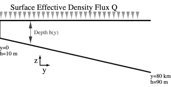
apply cooling over the entire domain, but assume a priori that the cross-shelf flow is capable of preventing convection from mixing to the bottom in all but a small portion of the domain. They run their laboratory experiments until this true.The simplest model of the response of shelf waters to cooling is a wedge shaped bathymetry with a surface heat loss that is uniform everywhere (figure 2.1). The forcing, geometry and flow are assumed not to vary in the alongshore direction. This model will be used to address the following questions:
Surface Effective Density Flux
Q
Depth h(v)y=o
h=10 mz
y=80 km
h=90 mFigure 2.1: The geometry and forcing of the model considered here.
What are the bulk effects of convection on the flow field, e.g. how can one represent the overall effect of many small convection cells?
- What does the flow field look like when the vertical mixing driven by cooling dominates the solution?
- When does the circulation prevent the cooling-driven mixing from mixing the entire water column?
- How does the circulation change when the cooling-driven mixing is prevented from mixing the entire water column?
These questions will be addressed both analytically and numerically. The nu-merical model used is SPEM 5.1, a rigid lid, Boussinesq, finite difference primitive equation model whose adaptation to this problem is described in the appendix. The equation of state for both the analytic and numerical work is linear, which allows the heat flux to be represented as a density flux. The geometry and cooling are chosen to be representative of the Mid-Atlantic Bight, which has a gentle bottom slope of O(10) and experiences winter time cooling rates of 0(200 W m-2) [Brown
and Beardsley, 1978; Mountain, Stout and Beardsley, 1996]. The cooling will be
rep-resented as a density flux,
Q,
of 7 x 10~6 kg m-2 s-1, which is equivalent to a heat loss of 170 W m-2 out of 100C water or 300 W m- 2 out of 30C water.2.2
The Parameterization of Convection
The dynamics of convection are non-hydrostatic and occur on horizontal scales of the same order as the water depth [Emanuel, 1994]. This work parameterizes the effects of convection in order to focus on the larger scale flow. The parameterization below gives vertical diffusivities of the same order as Mellor and Yamada [1982] and is used instead of Mellor and Yamada [1982] for simplicity.
A diffusive parameterization of convection implies eddy diffusivities which scale as the product of a convective length scale and a convective velocity scale. A rea-sonable length scale for the vertical mixing caused by convection on the shelf is the water depth. Given a buoyancy flux at the surface of gQ/po and the depth h, the only parameter with units of velocity one can assemble is
1
U* = -- Q (2.1)
PO.
In both atmospheric boundary layer experiments [Mellor and Yamada, 1982; Stull, 1988] and laboratory experiments with water [Fernando, Chen and Boyer, 1991;
Maxworthy and Narimousa, 1994], this scale has proven to be a good one for the
vertical velocity of a non-rotationally controlled convective region.
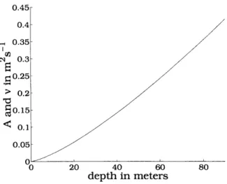
Using w* as a velocity scale and the water depth h as a length scale, a diffusivity for heat, v, and momentum, A, can be scaled as A = v = O(w*h). The constant of proportionality relating w*h to A and v will be assumed to be 0.25 hereafter in order to agree better with measurements of w presented in Mellor and Yamada [1982] and
0.45 0.4 0.35 0.3 0.25 > 0.2 0.15 20 40 60 depth in meters
Figure 2.2: The mass diffusivity and momentum viscosity as a function of water depth during unstable stratification for Q = 7 x 10⁻⁶.
mixing length is about the distance from a boundary, 0.5h is a good length scale.)
1 1
A = v = -w*h = -h3 --
Q
(2.2)4 4 PO
A density flux of
Q
= 7 x 10⁻⁶ kg m-2s-1 gives the diffusivities shown in figure 2.2.The generation of turbulence by the wind has been neglected even though it would be expected to increase the turbulent diffusivities. A 0.1 N m- 2 wind stress produces a turbulent velocity u* of
U* = = 102 m s1 . (2.3)
The free convective velocities w* from (2.1) range from 102 m s-1 in 20 meters of water to 2 x 10⁻² m s-' in 100 meters of water for the cooling used in this paper,
and so are of the same order as u*. It is unclear in the literature how the additional turbulence from the wind would be distributed through the water column, but if it
worked over the entire water column it could as much as double the eddy diffusivity. Since the scaling for v and A is only meant to be good to an 0(1) constant, the effect of wind-generated turbulence is less than the uncertainty of the convective diffusivity.
It is important to determine when rotation affects convection. Rotation ought not to affect convection when the time scale of convection, 2hw* 1 , is less than an
inertial period, 27f -. 2hw*1 is less than 2rf 1 when
h < Q (2.4)
2 pof 3'
Experiments bear out this depth limit, though the constant before (2.4) is often a
value other than (0.57)2 (about 2). Maxworthy and Narimousa
[1994]
find that theconstant should be 12.7, and Fernando, Chen and Boyer [1991] in their experiments find a value of 4.5.
This length scale is 700 meters for a mass flux of
Q
= 7 x 10⁻⁶ kg m-2 s1. Thus a convection cell in the the 10 to 100 meter ocean that is examined here will not feel the Earth's rotation.2.3
Flow Fields When Convection Reaches the
Bottom
When surface cooling is started in the homogeneous fluid of density po, convection quickly extends to the bottom. The fluid then has very high vertical mixing coef-ficients, and thus the two dimensional flow field is unable to transport significant heat across the shelf, and the heat balance is one dimensional (this will be justi-fied in section 2.4). The density field forced by a surface density flux
Q
is thusapproximately
p
Q=
+ po, (2.5)and the cross-shelf density gradient is
Op
Qtoh
(2.6)Oy
h
2ay
where t is the amount of time the cooling has been active and y is the cross-shelf direction. The time scale of the change in this density gradient is the time since cooling began, and the time it takes for the momentum dynamics to adjust to the density gradient is the much smaller diffusion time scale h
t
1 (of order hours). The momentum equations can thus be solved as if they were steady. The non-linear terms can be neglected because of the large spatial scale of the forcing. The equations of motion + UVu - fv = 4)
,A (2.7a) at Oz Oz + EVo + 1 + - (A ,v (2.7b)at
poay
+ Oz P = Po+ jgpdz (2.7c) vY + wz = 0, (2.7d)can then be reduced to
fv = 24 (2.8a) 1 IOP a ( 8v
fu
=+(A
A)
(2.8b) po Dy Oz Oz' PaPo+
P
z, (2.8c) Bywhere Po is the surface pressure.
The ratio of the Ekman depth, V2A/f, to the water depth varies from 4 to 1.4 for the viscosities given in (2.2) and the cooling rate used here of 7 x 10⁻⁶ kg m- 2 s-1. Since the Ekman depth is greater than the water depth, it would seem
that rotation could be ignored. However, if the forcing in one direction is greater than the forcing in the other direction this may not be true. This can be seen by scaling the equations with (where primes denote non-dimensional variables)
z = hz', (2.9a)
U U (uo 2 o'), (2.9b)
v = V v 2 v' , (2.9c)
where 3
E is the Ekman depth, U is the scale alongshelf velocity and V the scale
cross-shelf velocity. The parameter h2
/6
is assumed small, though when the results arecompared to full solutions, they are found to be reasonable even for h216 1 When the alongshelf and cross-shelf forcing are of the same order, and U V, the
equations can then be written in a non-dimensional form as
02U,
2 (2.10a)
h2 po gsj Op 02VI
0 = 0 zp + (2.10b)
VApo Oy VA&y &z'2'
to first order and with
02U/ V' (2.11a) U Oz'2' U h2 19p1 02V' n' = _ - + (2.11b) V' V.I/IApo Oy OZ'2'
as a second order correction. (PO' and Pol are surface pressure gradients associated with the first and second order solutions, and are not part of the forcing. They
will be found as part of the solution.) The boundary conditions for the first order equations are:
OU' x' h
0___ win dh
0_ _ ___in_ (Oq Z- 0 (2.12a)
0 Z UApo -0 - U' z = -h (2.12b) Oz A O0 - Wldh @ z 0 (2.12c)
OV'
rh " = v' z =-h (2.12d) Oz A 0 = o'dz, (2.12e)and for the second order equations the boundary conditions are:
Ou' = 0 (z = 0 (2.13a) rh -1 = C O z -h (2.13b) Oz A OV' = 0 @ z = 0 (2.13c) OV - rh @ (z= -h (2.13d) Oz A 4
0
= -oh'dz. (2.13e)The depth-integral of the cross-shelf velocity is zero by the combination of (2.7d) and no flow through the coast, and Tind and Tind are the along- and cross-shelf wind
stress respectively. The bottom boundary condition is a linear drag law. Because the windstress and density gradient forcing enter only in the first order equations, the non-dimensionalization indicates that the cross-shelf velocity will not be affected by rotation except for a correction of order h26- 2 of the alongshelf velocity, and similarly the alongshelf velocity will only be affected by rotation to an amount which scales as h2
6- 2 the cross-shelf velocity.
greater than V, (2.1Ob) and (2.11b) are no longer consistent because (U/V)*(h 2 )
will be order one. However, the solution to (2.10b) and (2.11b) can be summed in order to find a solution valid to within an error of h'/64uo. In this case the sum of the solutions to (2.10b) and (2.11b) represent the first order solution to the cross-shelf momentum balance, and implies cross-shelf velocities of order h2
/62uo.
The sum of the solutions to (2.10a) and (2.11a) are similarly valid even when the cross-shelf forcing is much greater than the alongshelf forcing.Because of the residual effects of rotation, rotation can only be neglected for a flow in a given direction if the flow in the orthogonal direction is much less than
h26E2 its strength.
The solutions to (2.10) and (2.11) are, in dimensional terms,
0
- O Dh-(g p h+ 3 +Twindh T h h2 h 2 Tx~awind h
6Apo Dy Apo Apo
9
g (P 3 1 OPO Twind 1 0 Ph2±Twin+
z +
z+
z+
h
-
Ol
+
6Apo y 2Apo Dy Apo r po Dy 2po Oy PO
1 POh2+ 9 'Ph 3Tindh
2ApO Oy 6Apo oy Apo .
h 2 z3 x2 A z2 1F x 4
\Tx-+2 wind 2 wid wind (
+
h)+
oE2
6Apo h2 2Apo r h r hpo r 2po_TX A'~ hrjxfd1 (h e 4 h' - wind +h) + J+± +O Uo +0 0 , 2Apo r 6ApO 64 6( (2.14) where S3h + Ah3 h2 +Ah) DPO Op 24 2r _ , 2 + Dy Oy~ 3 Ar ) wt 3 __ 2 3h4 +Ah 3 h 2 24 2r ) ind A 22h+ Ah2h + 2 E 3 r (2.15) h4 Opo E0 y
sections will be concerned primarily with the cross-shelf flow, and because the second order solution to the alongshelf velocity is algebraically formidable, only the first order solution will be given:
wsind 1 h h2 h 4
UO= "Z- -+ vo+ u (2.16)
Apo p Yr A 62
o
The analytical solutions for the density, the first order solution for the cross-shelf velocity v, and the full solution (2.14) are compared with a numerical model with no windstress (figure 2.3), and with a model with a 0.1 N M-2
(a
10m s-1) alongshore, downwelling favorable, wind stress (figure 2.4). There is an open boundary at the seaward edge that lets the flow leave the domain undisturbed, and it is described in the appendix to this chapter. The numerical model uses the same parameterization for convection as the analytical work when the convection mixes to the bottom. The numerical model agrees nicely with (2.14), even near the offshore boundary whereh2
/6
1. The cross-shelf order one solution, vo, which includes no rotational effects, predicts the cross-shelf velocity in the numerical model well when there is no alongshelf forcing, but both the first and second order solutions are needed when there is an alongshore windstress. When there is an alongshore windstress, the cross-shelf wind forced velocity is about one-quarter the alongshelf velocity at the seaward edge of the model.2.4
When Does Convection Not Mix the Entire
Water Column?
When convection extends through the water column, the flow is sluggish and the water is viscous and weakly stratified, incapable of driving a significant horizontal mass flux. Only when convection is prevented from mixing through to the bottom, and thus prevented from transmitting stress and buoyancy from the surface to the
No Wind Forcing
-
day 30
Numerical Model
Analytical Solutions
bS
30 0 -40[ 50 0-60 -70--80 0 10 20 30 40 50 60cross shelf distance, km
CIO
C0
0:
Figure 2.3: The solutions for the cross-shelf velocity and the density from (2.14), (2.5) and the numerical model. The bottom panel is the lowest order analytic solution for the cross-shelf flow. Dashed contours are negative.
0.1 N m-
2Downwelling Favorable Alongshore Wind day 30
Numerical Model
Analytical Solutions
CID
:
Figure 2.4: The solutions for the cross-shelf velocity and the density from (2.14), (2.5) and the numerical model. The bottom panel is the lowest order analytic solution for the cross-shelf flow. Dashed contours are negative.
bottom, can significant stratification form and a strongly rotationally affected cir-culation develop. Once this occurs, significant amounts of heat can be transported offshore (c.f. chapter 3).
In the atmospheric boundary layer, turbulent convection extends from the sur-face to where the air becomes stably stratified, and the mean stratification of the convective region is slightly unstable [Mellor and Yamada, 1982; Stull, 1988]. This is assumed to be true in the ocean, and the mean unstable stratification formed by the cooling is compared to the stable stratification formed advectively by the cir-culation to determine when convection mixes to the bottom. Once the water near the bottom is stably stratified, it is assumed that convection does not penetrate through it and the diffusivity in the stably stratified water is much reduced. (In the numerical models the diffusivity of heat and momentum of the stably stratified water are calculated according to a scheme by Pacanowski and Philander [1981], though other parameterizations yield comparable results. The diffusivity of any statically
unstable region is still given by 2.2.)
The unstable stratification formed by the cooling, pOoing, is found from the
system:
pt =(2.17a)
vpz = Q #z = 0 (2.17b)
Pz = 0 @z = -h (2.17c)
In the limit of time much longer than the time of a convective overturning, (h2V-),
and assuming the viscosity varies slowly compared to this time scale, the solution is
pcooling _Q (z + h). (2.18)
PZ hv
The solution for pcooling is valid even if v varies with depth. This is important, for more realistic parameterization of convection-driven mixing will prescribe mixing
that varies with, among other things, the distance from the wall and the local vertical stratification (including that forced by advective processes).
The stratification induced by the cross-shelf circulation near the bottom, padvec can be found from:
vpY = v'P (2.19a)
vPz = 0 @z =- h1,0. (2.19b)
This system of equations assumes that wpz, the vertical advective term, is negligible (which is justified below), and that the horizontal advection of density does not change the mean density of the water column, i.e. the heat/density balance is one dimensional. This is a good approximation when the depth mean density-flux divergence is much less then the density-flux divergence in most of the water column:
- vpydz < |vpy| .
(2.20)
/I _h
Since the depth integral of v is zero to enforce no flow through the coast, this can be scaled as
| hvpyz|
<
VPy. (2.21)Substituting (2.18) and (2.5) into (2.21) gives
t 1
< - (2.22)
h2 V
This is easily true for h ~~ 50m, t ~ 106s, and v ~ 0.1m2 s-1. The advectively
the bottom, again assuming that pyz 0, to get
p vdz = v padvec
(2.23) YZ
6-h
where 6 is an arbitrary height above the bottom. To compare this result near the bottom with the stratification from cooling, the integral of v must be approximated. The Taylor series approximation
vdz
=6 vz=-h+6(2.24)
is accurate near the bottom if a stress condition is used as the bottom boundary condition for the momentum equation. An example stress condition is
Av, = rv @Q) z = -h, (2.25)
where r is the bottom linear drag coefficient. Near the bottom, the length scale of velocity change is A/r, which for realistic values of A (10-3 to 10-1 m2 s-) and
r (10-4 m s-1) gives length scales of tens to thousands of meters, depending on whether the water column is stable or not. (This does not mean that the boundary layer extends that far, only that there is a region near the bottom where v is ap-proximately constant). If near the bottom a log-layer boundary condition is used, (2.24) has a slightly different interpretation but is till approximately valid. In the log-layer, the velocity profile is
Vu
+
In
,
(2.26)
K
z
0 I1988, p. 376]. Equation (2.24) is then tantamount to approximating
I
o-h
vad z ~ 6 Vu =6.hIntegrating (2.26) directly and taking the ratio of the integral and (2.27) allows one to estimate the error caused by neglecting the log layer:
V/6z-6h
(i-h
vudz) (2.28)Assuming 6 im and z0 ~O0cm, this ratio is about 1.16, indicating that (2.24)
over-estimates the transport by about 16%. The stratification formed by advection near the bottom, (2.23), can now be written with (2.24) as
advec - 6PY z=6-h (2.29)
PZ-h - V (.9
Again, this solution is valid even if v varies with depth.
At this point the assumption that wpz is negligible compared to Vpy can be checked. w is scaled as
W = 0 V ,h (2.30)
so wpz is much less than Vp, when
Py
>h
pz. (2.31)Substituting (2.29) for pz and rearranging the resulting equation leads to
(z + h)v oh
1 > , (2.32)
V hye
which is easily true for the cases presented here where v is 0(10-2 m s-'), Oh/Dy is
(2.27)
O(10-3) and v is O(10-' to 10- 3m S2).
The total stratification forced by the cooling and advection is, near the bottom and from (2.18) and (2.29),
- = - - h + . (2.33)
19z g, p 6-h O h
The water column is thus stably stratified near the bottom when
Op
Q(234)
Oy h I
which is when the divergence of the advective flux of density is greater than the divergence of the density flux caused by cooling. This can be solved for the minimum velocity needed to make the water stably stratified near the bottom, vc,
c
=
Q
y)
(2.35)
This can then be written
Vc ( h7 (2.36)
t Oy
with ap/&y from (2.6). Once the cross-shelf velocity near the bottom exceeds v, convection cannot reach the bottom, so the enhanced mixing due to convection cannot reach the bottom. The velocity vc should be compared with the velocity either at the bottom, when A is constant, or at the top of the log-layer, when there is one. The diffusivity of density, v, does not enter into (2.35) or (2.36) because both the unstable stratification forced by the cooling, (2.18), and the stable stratification forced by the circulation, (2.29), scale linearly with v'. It takes a smaller cross-shelf velocity to make the water stably stratified as time increases because as time increases the cross-shelf density gradient increases, increasing the stabilizing stratification caused by a given cross-shelf velocity (2.29).
To test the criterion (2.36), five numerical model runs were made, each with the same geometry and surface cooling as previously described, and each with initially homogeneous water. The model uses the exact same vertical viscosity and density diffusion as the analytic work. In one model run , no wind forcing was used, and in the other four an 0.1 N m-
(~
10 m s-1) wind was applied in the onshore, offshore, or one of the alongshore directions. The cross-shelf velocities near the coast in the model within 0.3 days of the onset of stable stratification are plotted in figure 2.5 after being scaled by (2.36). All five models first become stratified near the coastal boundary, and in all five cases the scaled cross-shelf velocity is very nearly one where the water becomes stably stratified. Thus (2.35) and (2.36) are good measures of when the cross-shelf current can prevent convection from reaching the bottom.In section 2.3, an analytic solution was found which predicted the flow fields of the numerical model well, and in this section a criterion was found for the cross-shelf velocity needed to make the water column stable. It is possible to combine equations (2.14) and (2.36) to provide an expression for the onset of stable stratification in the model, but the result is algebraically formidable. However, in the limit of Ar-1
>
h,the near bottom velocity can be written as:
v = _ot h3 g Op f Thrd in (2.37)
2A (
24A Oy Apo 6Apo
This scale for the bottom velocity is compared with the velocity from the numerical model, the full analytic solution (2.14), and the criterion for the onset of stability (2.36) in figure 2.6. The velocity scale Vbot compares well with both the
numeri-cal model and (2.14), and when these three estimates of the near bottom velocity exceed (2.36) the increased cross-shelf currents associated with the onset of stable
Scaled Cross-Shelf Velocities
Shaded where v/vc > 1
-10 -15 -20 6625 -30 -35 0 5 10 15 20cross shelf distance, km
10 15 20
cross shelf distance, km
25 30 0 -5 -10 15 5-20 L25 -30 -35 25 30 4 ..0.5 QS 0
Day 48.0
I 5 10 15 20 cross shelf distance, km10 15 20
cross shelf distance, km
Figure 2.5: Scaled cross-shelf velocity just before convection is prevented from mixing to the bottom for five model runs with different wind forcing. The arrow indicate the direction of the wind relative to the coast. Only the inner 30 km of the model domain are shown. -0.5 Day 35.4 -5 -10 +-15 5-20 6.25 -30 -35 25 30 ®
Cross-Shelf
Bottom Velocity Where Water First Becomes
Stable, 3km offshore
0.01
0009 No Wind Where the numerical model 0.008- velocity suddenly increases, 0.007- the water has become stable
0.006- Numerical Model --- Analytic Solution .004 V t 0.003 V 10 20 30 days 0.008 0.007-0.006 ~0.005 -0.004 -0.003 10 20 30 40 50 0 10 20 days days . 0.01r ________
I.0.009
-... 0.008- 0.007-0.006 0.005 0.004-0.003F 0.002 S0.001 C bat 10 20 30 40 50 40 50 60 70 days days 30 40 50 80 90Figure 2.6: The cross-shelf bottom velocity for the five numerical model runs shown in figure 2.5. the velocity is computed 3km offshore, where the model first becomes stable. The thin vertical line marks where vc = Vbot, the criterion for stability given in (2.38). The sharp increase in the cross-shelf velocity in the numerical model indicates the onset of stable stratification near the bottom. The arrows represent the wind direction relative to the coast. 0.01-0.009 0.008 0.007 0.006 '00.005 0.004 0.003 0.002 0.001 V ... ... III#
'Wmw
*
stratification are seen.1 The velocity scale Vbot exceeds ve when
gQ
oh 2 h2+ x Oh Y h
gqQ
N
2 ±hfTwind fD (U Tind D= - ** t. (2.38)
24Apo Oy 24A2PO Oy 6Apo Oy
The time for the onset of stability can be found by solving (2.38) with the quadratic equation. These times are marked in figure 2.6. From (2.38) it can be seen that the water will become stable where A is the least. When the mixing is driven by the cooling alone and increases as the four thirds power of depth, (2.2), this occurs where the water is shallowest (in the numerical model stability first occurs 3 gridpoints (or 3 ki) from the coastal wall because of the boundary layer associated with the coastal wall). However, in a real ocean the mixing may increase as the water gets shallower (if, for instance, the mixing is driven by surface gravity waves), so this result may well break down as the water becomes shallow. Furthermore, (2.38) depends on a cross-shelf gradient of density which increases as h 2, (2.6). As the water become shallower and the cross-shelf density gradient increases, it is likely that some form of lateral mixing would reduce the gradient, reducing the effectiveness of advective restratification and moving the location of the first stable stratification offshore. Equation (2.38) also illustrates that an alongshelf wind is less able to make the water stable than a comparable cross-shelf windstress by a factor O(h2
/6),
because the alongshelf wind generates a cross-shelf current that is O(h2/61)
weaker than an equivalent cross-shelf windstress. The importance of adensity-driven circulation relative to wind-driven circulation is seen to increase with time, because the strength of the density driven circulation increases in time while the wind driven circulation remains steady.
'The velocity in the numerical model exhibits small At noise, which is damped every 3.6 days
In the absence of wind, the water is predicted to become stable by (2.38) when
24Apo (Bh -1
t =y) (2.39)
gqQ Oy
38.4 days for the no wind case.
The numerical model becomes stable at about 39.9 days, and the discrepancy arises not from the failure of the scale for v but, as can be seen from figure 2.6, from the approximation of the bottom velocity by (2.37). An 0.1 N m 2 alongshore windstress drives cross-shelf velocities of about 10-m s-. This retards the onset
of stable stratification by 8.1 days when the alongshore wind is upwelling favorable, and advances the onset by 4.5 days when the wind is downwelling favorable. The change in time from the no wind case is unequal because, as can be seen from (2.38) and figure 2.6, vc scales as t-1, so reducing the bottom velocity by a constant changes the time when V =Vbot by more than increasing the bottom velocity. An 0.1 N m 2 cross-shelf wind drives cross-shelf currents almost seven times greater
then the equivalent alongshelf windstress, and so changes the time of the onset of stable stratification by more than the equally strong alongshelf wind. An offshore wind retards the onset of stable stratification by 49.5 days while an onshore wind advances it by 21.9 days.
The solution for the near-bottom velocity needed to make the water stably strat-ified does not depend on the magnitude or shape of the eddy viscosity A or density diffusion v except to the extent that a vanishing eddy viscosity near the bottom introduces errors into (2.24), and these errors are shown to be small in (2.28). The estimates of the actual cross-shelf velocity in (2.37) and (2.14) do, however, depend on the magnitude and the vertical profile of A. From the expression for V 7t, (2.37), the effect of changing the magnitude of A can be estimated: the cross-shelf flow driven by cross-shelf winds and density gradients scales as A-, and the cross-shelf flow driven by alongshelf winds scales as A .
The cross-shelf velocity profile also depends on the vertical structure of 4. Ob-servations of the turbulent velocity for free convection find that it varies with height above the boundary and goes towards zero at the boundaries [Mellor and Yamada, 1982; Stull, 19881. Realistic mixing schemes account for this by varying A with the distance from the boundary. The level 2 turbulence closure presented in Mellor and
Yamada [1982] varies the mixing approximately quadratically, so that
A oc - z (z + h) (2.40)
h
[Nunes Vas and Simpson, 1994]. Another approach which has been used is to assume
that the vertical mixing varies linearly with distance away from the wall,
A oc w*( _ z + - (2.41)
(2 2
which could be regarded as an extension of the log-layer throughout the water column. These and other schemes are presented and discussed in the context of wall-generated turbulence by Lentz
[1995]
((2.40) reduces to the cubic case in Lentz whenw* is used to scale the turbulent velocity). To get a rough idea of the sensitivity of
the near bottom velocity to the vertical profile of A, the cross-shelf velocity is found for the two profiles given in (2.40) and (2.41), and for a constant eddy viscosity. Each will be normalized so the depth average A will be 0.25w*h, as in (2.2). Since the viscosities in (2.40) and (2.41) go to zero at the bottom and top, the full numerical model cannot be used to solve for the velocity profiles. Instead, (2.10) is solved by a Runge-Kutta solver with the boundary conditions
Ov
= 0 @z = -zO, (2.42a)
V 0 Cz = -h + zo, (2.42b)
[Lentz, 1995]. Herein, zo = 10- 2m. The constant eddy viscosity solution is that of
(2.14), and as long as Ar-
>
h, it is not sensitive to the value of r. Figure 2.7shows A and the cross-shelf velocity for the three vertical eddy viscosity profiles. The cross-shelf velocities in 13 meters of water are found for day 39.6 of the no wind case, which is where and just before the water column becomes stable in the vertically uniform A case. The only qualitative difference in the cross-shelf velocity profiles is at the bottom, where the velocities in the depth variable A cases go to zero in a log-layer. This is caused by the boundary condition (2.42), and as discussed above v is then compared to the velocity many zo above the bottom. The velocity one meter above the bottom, which is approximately where the peak cross-shelf velocities occur in the depth dependent A cases, is about 30% lower than the near bottom velocities in the constant A case. The velocity is about 12% lower when A is given by (2.40) then when given by (2.41). (In both cases (2.28) accurately predicts the error in (2.24), about 18%.) Since the changes in the near bottom velocities for the more realistic mixing profiles are relatively small, it seems reasonable to use (2.37), (2.2), and (2.35) to estimate the time for the onset of stable stratification in the ocean. In a case with no wind, a 30% reduction in the near bottom cross-shelf velocity implies a 20% increase in the time until Vbot > vc and the water column
becomes stable (2.39).
2.5
When Convection no Longer Mixes to the
Bottom
When convection extends to the bottom, pressure gradients and wind forcing can be balanced directly against bottom friction. Once the velocity near the bottom exceeds
v, and convection no longer mixes to the bottom, the viscosity near the bottom is
reduced to levels appropriate for neutral and stably stratified waters. This allows rotation to affect the circulation strongly. Wind will then force a transport to the