J L
DOCENT ROOMD-E BOOM 36-43iRESFARH LABRATrRY OF ELECTRONICS MASSACHU 'r! TI t"'ITE OF TECHNOLOGY... CAKBRIDGE 33 l/ -, CirlU ETS, U S.A.
DESIGN PROBLEMS IN PULSE
TRANSMISSION
DONALD WINSTON TUFTS
TECHNICAL REPORT 368
JULY 28, 1960
MASSACHUSETTS INSTITUTE
OF TECHNOLOGY
RESEARCH LABORATORY OF ELECTRONICS CAMBRIDGE, MASSACHUSETTS
_I___
I
I_
__
_ _
___
_
_
The Research Laboratory of Electronics is an interdepartmental laboratory of the Department of Electrical Engineering and the Department of Physics.
The research reported in this document was made possible in part by support extended the Massachusetts Institute of Technology, Research Laboratory of Electronics, jointly by the U. S. Army (Sig-nal Corps), the U.S. Navy (Office of Naval Research), and the U.S. Air Force (Office of Scientific Research, Air Research and Develop-ment Command), under Signal Corps Contract DA36-039-sc-78108, Department of the Army Task 3-99-20-001 and Project 3-99-00-000.
MASSACHUSETTS INSTITUTE OF TECHNOLOGY RESEARCH LABORATORY OF ELECTRONICS
Technical Report 368 July 28, 1960
DESIGN PROBLEMS IN PULSE TRANSMISSION
Donald Winston Tufts
Submitted to the Department of Electrical Engineering, M. I. T., May 25, 1960, in partial fulfillment of the requirements for the degree of Doctor of Science.
Abstract
Criteria for determining optimum pulse shapes for use in a synchronous pulse trans-mission link are proposed and compared. Formulas for the optimum pulses are pre-sented, and calculations are carried through in examples.
In a secondary problem, we present methods for calculating optimum interpolatory pulses for use in reconstructing a random waveform from uniformly spaced samples. The case of a finite number of samples and the case of an infinite number of samples are discussed. A mean-square criterion is used to judge the approximation. The results provide a generalization of the sampling principle.
TABLE OF CONTENTS
I. Introduction 1
II. Thin Pulse Performance Criteria 2
The Basic Model 2
Definition of Interpulse Interference 4
Discussion of the Basic Model 5
Output Energy Criterion 6
Weighted Output Energy Criterion 8
Least Squares Criterion 11
III. Low Error Probability Performance Criterion 15
Introduction 15
Low Error Probability Criterion for a Noiseless Link 15 A More Explicit Expression for the Low Error Probability
Criterion 18
A Necessary Condition for an Optimum Transmitted
Pulse Shape 22
Optimum Pulse Shapes for a Noiseless Link 25
Low Error Probability Criterion for a Noisy Link 29
Necessary Conditions for Optimum Pulse Shapes in a
Noisy Link 31
Optimum Pulse Shapes for a Noisy Link 35
IV. Reconstruction of a Random Waveform from Uniformly
Spaced Samples 40
The Problem 40
The Case of a Finite Number of Samples 41
The Case of an Infinite Number of Samples 45
I. INTRODUCTION
This report is concerned with problems in the design of synchronous pulse trans-mission links like the link shown in Fig. 1. In this model the transmitter sends a vol-tage pulse into a transmission line every T seconds. The pulses differ only in their
amplitudes and time delays. The peak amplitude of each pulse corresponds to a mes-sage. If the peak amplitude of a transmitted pulse can be determined at the receiver, then the message carried by that pulse can also be determined.
PULSE TRANSMISSION FILTERING MESSAGE
MESSAGES TRANSMITTER LINE NETWORK DETECTOR MESSAGES
[ L- N RECEIVER
Fig. 1. Block diagram of a synchronous pulse transmission link.
The receiver consists of a linear network and a detector. The output of the trans-mission line is filtered by the linear network, and the detector operates on the resulting waveform every T seconds to extract one message. Ideally, the time delay between the transmission of a message and its detection is a constant. That is, the link is syn-chronous.
Our main problem is to determine transmitted pulse shapes and linear filtering net-works that optimize the performance of such links. A secondary problem is to find opti-mum interpolatory pulses to use in reconstructing a random waveform from uniformly
spaced samples. The same mathematical methods are required in each problem because the same type of nonstationary waveform occurs.
Our main problem is motivated by the following practical, theoretical, and mathe-matical considerations.
1. Synchronous pulse links are of great practical importance (1, 2) because they are naturally suited to the transmission of digital messages (3). We discover how signal power and bandwidth can best be used in our models to obtain good link performance.
This is a step in attempting to improve present synchronous pulse links (1).
2. It has been shown that, under idealized conditions, pulse code modulation (PCM) exchanges increases in bandwidth for decreases in signal-to-noise ratio more efficiently than comparable systems, such as frequency-modulation systems (4). A PCM link is a
special form of the synchronous pulse link. It is of interest to discover how well the theoretical advantages of pulse code modulation are preserved in link models that are
different from the model that is considered by Oliver, Pierce, and Shannon (4). 3. The random waveforms that occur in synchronous pulse links are members of nonstationary ensembles. The mathematical properties of these waveforms have been only partially explored (5, 6, 7).
Our search for optimum interpolatory pulses is also motivated by mathematical interest in nonstationary ensembles. However, the main motivation is provided by two questions: How well can a random waveform be reconstructed from uniformly spaced samples of the waveform? Can present methods of interpolating samples be used for a wider class of random processes?
In answering the first question, we shall obtain estimates to a measure of the optimum reconstruction by considering a particular method of reconstruction. The pres-ent methods that are referred to in the second question are those discussed by Shannon and others (8, 9). Shannon considered the exact reconstruction of bandlimited waveforms from an infinite number of samples. We shall consider the approximate reconstruction of random waveforms from a finite number of samples.
II. THIN PULSE PERFORMANCE CRITERIA
2. 1 The Basic Model
Let us use the block diagram of Fig. 2 as our basic synchronous pulse transmission link model - a model that follows Shannon's model for a general communications system
(10). The message source produces a sequence of area modulated impulses, m(t), where
00oo
m(t) = an u(t-nT) (1)
n=-oo
and u (t) is the unit impulse or delta function. Each real number an, n = 0, ±1, 2,. corresponds to a transmitted message. For example, a particular message might be a page of English text or it might be a voltage amplitude. The waveform m(t) is the input for the linear pulse-forming network of Fig. 2, which has an impulse response s(t) and a transfer function S(f). Its output is
00
fI(t) = E an s(t-nT) (2)
n=-oo
The waveform fI(t) represents the transmitted signal in a real synchronous pulse link. The linear transmission network represents the transmission medium in a real link. It has impulse response (t), transfer function L(f), input fI(t), and output
00oo
fs(t) = an r(t-nT) (3)
n=-oo where
r(t) = / s(u) f(t-u) du (4)
The pulse r(t) is the response of the transmission network to an input pulse s(t). The detector consists of a sampler and a clock. Ideally, the clock output, c(t), is
a periodic train of unit impulses. And, ideally, each clock impulse coincides with a peak value of one of the pulses of fs(t). An instantaneous voltage sample of fs(t) is taken whenever the sampler receives a clock impulse. The ideal clock impulses and three typical pulse components of fs(t) are depicted in Fig. 2. It is assumed that r(t) attains
H-
DETECTOR
-JTPUT Sn m(t) = an U (t-nT); fI(t) = an (t-nT); fs(t) = anr(t-nT) n -C n z.0D nz-CD r(t)= s (u) (t-u)du -alMESSAGE SOURCE OUTPUT m(t) AREA, -0 D ·* -T 0 T PULSE COMPONENTS OF f(t) -/'ar t 'a r(t+T) (b-I)T bT (b.I)T O (b-I)T bT (bI)T · * * t=+O
IDEAL CLOCK IMPULSES
.c(t) AREA.
-T O T
· · · t=+ca
IDEAL SAMPLER OUTPUT a | r(bT)
al r(bT)
aO r(bT)
--O (b-I)T (bT) (b+l)T
Fig. 2. Basic synchronous pulse transmission link model and associated waveforms.
-a,) * * t
I
a peak value when t = bT, where b is a positive integer. Thus, if the clock emits the ideal impulse train shown in Fig. 2 and if we say that the pulse an s(t-nT) is transmitted at time nT, then the time delay between transmission and detection of a message is bT seconds.
The actual time delay is a random variable because we assume that there is jitter in the actual sampling instants. More specifically, the actual sampling instants are assumed to be in one-to-one correspondence with the ideal sampling instants. Each actual sampling instant does not differ from its corresponding ideal sampling instant by more than P seconds; and 2P is smaller than T, the time between ideal samples. Physically, this might come about because of thermal noise in the clock's oscillator. Any long-term drifting of the clock impulses in either time direction is assumed to be prevented, for example, by the use of special retiming pulses that are sent through the transmission network.
2. 2 Definition of Interpulse Interference
If the clock impulses were ideal and r(t) were zero at all ideal sampling instants, except t = bT, then the sampler output would be a sequence of real numbers, {an r(bT)}, that are proportional to the message sequence {an}. Three elements of an ideal output sequence are shown in Fig. 2. We denote the actual sequence of sampler outputs by {sn}. We say that our link performs well if each element of the normalized sampler
output sequence r(b) is close to the corresponding element of the message sequence r(bT)
{an}. The differences n - an , n = 0, ±1,± 2,. .. , are called interpulse interference.
r(bT) n
Thus, the link performs well if interpulse interference is small.
Using this definition of interpulse interference, our assumptions about the sampler operation and the sampling time jitter, and the expression for the sampler input in Eq. 3, we can write the interpulse interference more explicitly. At any particular sampling instant, ts, the interpulse interference is
00 E aj r(ts-jT) - an r(bT) J=_00 I(t ) =(5) r(bT) where (b+n) T - < ts < (b+n) T + (6) n = 0, 1,2,... (7)
and 2, the extent of the time uncertainty interval about each ideal sampling instant, is less than T. We recall that 1/T is the rate of transmitting mes-sages.
2. 3 Discussion of the Basic Model
In previous publications on synchronous pulse transmission, ideal clock impulses are almost always assumed (11, 12, 13). Under this assumption one can choose a band-limited received pulse r(t) in such a way that r(t) is zero at all ideal sampling instants except t = bT. Under these conditions the interpulse interference, I(ts), is zero at all sampling instants. This occurs, for example, when
sin[(rr/T)(t-bT)]
r(t) = (8)
(rr/T)(t-bT)
In the absence of noise such a link would perform perfectly. That is, the output sequence of samples would be proportional to the input message sequence of amplitudes. However, the models of references 11, 12, and 13 do contain noise sources. In those papers major emphasis is placed on combating noise other than interpulse interference. Here, we place our emphasis on reducing interpulse interference. We assume that the effects of any additive noise source, such as that shown in Fig. 3, are negligible, compared with the interpulse interference. By the effects of the noise we mean the perturbations of the normalized sequence of samples that are due to the noise alone. If the noise source is removed, the linear filtering and transmission networks of Fig. 3 can be combined, and we have our basic model of Fig. 2. It can be seen from Eq. 5 that interpulse inter-ference is independent of the amplitude of the standard input pulse s(t). This follows
from the fact that the amplitude of the received pulse r(t) is proportional to the ampli-tude of s(t). But if the amplitudes of the received pulses are increased by transmitting
larger pulses, the effects of the noise are reduced.
Fig. 3. Modified basic model.
Let us use our model of Fig. 2 and assume that the transmitted signal power is so large that, for a given rate of signaling, 1/T, the performance of the link is limited only by interpulse interference. For rapid rates of signaling this behavior can be achieved at a level of signal power that is small, compared with the level required at slow rates. This comes about because interpulse interference increases with the rate of signaling, due to greater received pulse overlapping, while the noise effects are inde-pendent of the signaling rate.
2. 4 Output Energy Criterion
For a given rate of signaling we wish to make the interpulse interference, I(ts), small at all sampling instants so that the link will perform well. We also desire to signal as rapidly as possible so that our rate of flow of information is high. However, we do not attempt to signal so fast that the condition
2P < T (9)
is violated. We recall that 2 is the extent of the sampling time uncertainty interval that surrounds each ideal sampling instant, and 1/T is the signaling rate. Inequality 9 preserves the synchronous property of our basic link model.
One way to make I(ts) small while signaling at a rapid rate is to make each pulse as thin as possible. This can keep pulse overlap small. A criterion for obtaining a thin
output pulse is that
C 1 0 [r(t)]2 dt (10)
1 r(bT) -oo
shall be small. We assume that
r(bT) =
f
s(x) (bT-x) dx = K1 (11)where K is a constant. As before, r(t) is to attain a peak value at t = bT, and b is a positive integer. It is reasonable that, if the energy in a pulse is small for a prescribed peak value, the pulse must be thin. Strictly speaking, C1 is proportional to the energy
delivered by r(t) only if the impedance seen by r(t) is pure resistance. Further inter-pretation of C1 is given in section 2. 6.
Standard calculus of variations and Fourier methods can be used to show that
2S(f) I L(f)12- kXL(f) exp(-j2rrbTf) = 0 (12)
is a necessary condition for C1 to be minimized by variation of S(f), subject to the con-straint of Eq. 11. (See ref. 14.) These methods are illustrated by a more detailed derivation in section 2. 5. We recall that S(f) is the Fourier transform of the input pulse s(t); L (f) is the complex conjugate of the transfer function of the transmission network; and X is a Lagrange multiplier (14).
Equation 12 implies that IS(f) can become arbitrarily large near a zero of L(f). For example, if
|L(f)| = exp(-f 2 ) (13)
then
IS(f) = exp(f2) (14)
Imposing a constraint on the input energy per pulse is a natural method of avoiding this difficulty. In the case of statistically independent messages the input energy per pulse is proportional to the average transmitted power. In other cases it is a convenient measure of average power. For economic reasons it is often important to use average power efficiently.
If the input admittance of the transmission network is Y(f), and s(t) is a voltage pulse, then the equation
S(f) Y(f) S*(f) df = K2 (15)
0o
states that the input energy is a constant K2. If Y(f) is a constant conductance, then Eq. 15 becomes
f
S(f) S (f) df = K2 (16)0o
A necessary condition for C1 of Eq. 10 to be minimized by varying S(f), subject to the constraints of Eqs. 11 and 16 is
*
kL (f) exp(-j2rrbTf)
S(f)= 2 (17)
I
L(f) 12 + 1where and are Lagrange multipliers that must be chosen to satisfy our two con-straints. Equation 17 has the advantages that S(f) is Fourier-transformable and its mag-nitude is bounded. One might think that values of . and X could be chosen to offset these advantages. However, such values lead either to infinite input pulse energy or to negative values of IS(f) .
If we select the values K1 and K2 arbitrarily, we have no guarantee that we can solve the constraint equations 11 and 16 for p and . But, given any pair of real numbers
([i, X), we can compute K1 and K2. We can then vary p. and to bring us closer to the desired values of K1 and K2. This is a reasonable procedure because S(f), and hence K1 and K2, are continuous functions of and ip.
As an example, let us assume that
(exp(-j2rbTf) ifl < B
L(f) = (18)
otherwise
Then, from Eq. 17, we have
\/4+1
If < B
S(f):= (19)
H s = 2BX sin 2Bt (20) s(t) + 2TrBt(20)
And r(t), the Fourier transform of R(f) = S(f) L(f), is 2BX sin 2rrB(t-bT)
r(t) + 2 B(t-bT(21) 27rB(t-bT)
From Eqs. 11 and 21, we obtain 2BX
r(bT) = K (22)
+1 1 1
By use of Eqs. 16 and 19, we have
S(f) S*(f) df = 2B = K2 (23)
Since K1 and K2 are both determined by the ratio X/p.+1, they cannot be chosen independ-ently.
If we had used the constraint of Eq. 15, rather than the constraint of Eq. 16, then Eq. 17 is replaced by
*
XL (f) exp(-j2rbTf)
S(f)= (24)
S(f IL(f) 12 + Re[Y(f)] (4)
Since Eqs. 17 and 24 appear as special cases of Eq. 46, we postpone additional inter-pretation to section 2. 6.
2. 5 Weighted Output Energy Criterion
We shall now consider a second measure of pulsewidth. It is
C
r(bT)
J (t-bT)2 [r(t)]2 dt (25)r(bT) -o
This measure puts greater emphasis on portions of the pulse that are far away from the sampling instant t = bT. According to this measure, r(t) is concentrated at t = bT if C2 is small. The quantity C2 is analogous to the variance of a probability density func-tion (15).
We shall now minimize C2 under the constraints of Eqs. 11 and 16. Expressed in the frequency domain, we want to minimize
C2 1
/
d IR(f) exp(+j2rrbTf) 2 df (26)r(bT) -oo df
by varying S(f), subject to the constraints Hence,
oo
r(bT) = R(f) exp(j2rrbTf) df = K1
from Eq. 11 and
from Eq. 11 and
-00
(27)
(28) IS(f) 2 df = K2
from Eq. 16.
The purpose of Eqs. 11 and 27 is to guarantee that our received pulses are large enough so that the effects of noise are negligible compared to the interpulse interference. The purpose of Eqs. 16 and 28 is to conserve the average transmitted power.
Equation 26 can be written more explicitly as
2 (T
r(bT) oo
d IR(f)l] +
[IR(f)l
F
df
(29)where p(f) is the phase function of R(f) exp(j2rrbTf). Note that the second, positively contributing term of the integrand in Eq. 29 is zero if p(f) is a constant. This constant must be zero or, equivalently, a multiple of 2r. Otherwise, r(t) would be a complex
function of t. We also note that the first term of the integrand in Eq. 29 is independent of p(f). Thus, we should choose pS(f), the phase function of S(f), in such a way that
p(f) = pR(f) + ZrrbTf = PS(f) + pL(f) + 2rTbTf = 0 (30) where pR(f) and pL(f) are the phase functions of R(f) and L(f).
transmission network transfer function. We now want to minimize
We recall that L(f) is the
C2 r(bT)
f
L
I S(f)L(f) I df by varying S(f) , subject to the constraintoo
r(bT) =
I
S(f)R(f) df = K1 ·i··i;-oo(31)
(32)
and the constraint of Eq. 28. Using a well-known theorem of the calculus of variations, we can solve our problem by minimizing
f
.([ d IS(f)L(f) ] - XIS(f)L(f) - .IS(f)I} dfoo
(33)
subject to no constraint (16). The Lagrange multipliers, such a way that Eqs. 28 and 32 are satisfied.
Minimization of integral 33 by variation of S(f)
X and 1±, must be chosen in
problem (17). A necessary condition for such a minimum is that I S(f) I must satisfy the differential equation
d2
1L(f)I
d2S(f)L(f):
=
XL(f)I
+
I
S(f)
(34)
df
The optimum phase function PS(f) for S(f) must satisfy Eq. 30. That is,
PS(f) + PL(f) = -2rbTf (35)
The writer has not obtained a general solution for Eq. 34, but special cases have been considered.
Let us remove our constraint on the input pulse energy by letting [ = 0. We also
assume that the transmission network is an ideal lowpass filter as in section 2. 4 (cf. Eq. 18). Thus, Eq. 34 becomes
2 2
d
2 Is(f)L =
z
I R(f) =IfJ
<B (36)df2 df
or
IS(f)L(f)l = R(f)I = f2 + K3
If!
< B (37)where K3 is a positive constant. There is no first-degree term in R(f) I; from Fourier integral theory, I R(f) I must be an even function. From Eqs. 35 and 37 a solution is
R(f) =
d exp(-j2nbTf) If < B
(38)
otherwise and
= 2 sin 2rrB(t-bT) sin 2iB(t-bT) cos 2rrB(t-bT)
r(t) = 2B(XB2+K3) - 4kB 3 2 (39)
3 2SB(t-bT) [2TrB(t-bT)]3 [2TrB(t-bT)]2
If k is chosen to be negative and K3 chosen to be -XB2, then the first term of r(t) drops out, and r(t) falls off as /t2 for large t. In this case, L'Hospital's rule shows that
r(bT) =- B3 = K1 (40)
Thus, our constraint can be satisfied for any positive K1.
Gabor's "signal shape which can be transmitted in the shortest effective time" is a particular solution of Eqs. 34 and 35 when there is no constraint on r(bT); that is, = 0, and L(f) is again an ideal lowpass transfer function. In this case
K4 cos (rf/2B)
If
< BS(f) = (41)
where K4 is a constant. It follows that K4 cos 21Bt
s(t) = r(t+bT) = 2 2 (42)
v B[(1/4B )-4t
]
We note that the envelope of this pulse falls off as K4/4rBt2 for large values of t. For comparison, a pulse whose spectrum has the same bandwidth and peak value is
2BK4 sin rBt
sl(t) = 2 (43)
(rrBt)
The envelope of sl (t) falls off as 2K4/Br 2t2, or slightly slower than the pulse s(t) of Eq. 42. However, sl (t) has a larger peak value than that of s(t).
2. 6 Least Squares Criterion
The thin pulse criteria were chosen to reduce the effects of pulse overlap. They both neglect an effect of sampling time jitter. For example, if the received pulses are very thin it is possible that a sample is taken when no pulse is present. In short, a good received pulse must not only have low amplitude when other pulses are sampled, but also have high amplitude whenever it can be sampled.
We continue to assume that each sampling instant occurs within p seconds of an ideal sampling instant and that 2 is less than T, the time between pulses. Thus, a desired received pulse-shape is
(d bT- <t <bT +
d(t) = (44)
LO otherwise
where d is a positive real number that is chosen to satisfy our requirement for received pulse amplitude. We recall that this amplitude must be large so that we can neglect the
effects of noise and use our model of Fig. 2. As before, we assume that the transmis-sion delay is bT seconds.
Our criterion for a good received pulse is that
2 ,,,,_,,,,,·,,(45)
CB =_ [d(t)-r(t)]2 dt (45)
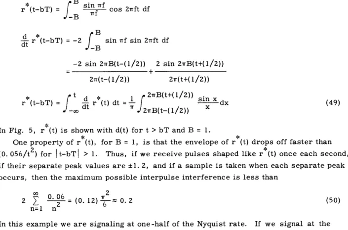
shall be small. A necessary condition for C3 to be minimum by varying S(f), the Fourier transform of the input pulse shape s(t), is
D(f) L*(f)
S(f)= (46)
L(f) 2 + pRe[Y(f)]
This condition is obtained by the standard Fourier and variational techniques that we employed in section Z. 5. The total energy available from a transmitted pulse is con-strained as in Eq. 15, and the Lagrange multiplier [i must be chosen to satisfy this
constraint. The Fourier transform of the desired pulse shape d(t) is denoted by D(f); L (f) is the complex conjugate of the transfer function L(f); and Re[Y(f)] is the real part of the input admittance of the transmission network.
Equations 17 and 24 can be considered as special cases of Eq. 46 because the mathe-matical steps leading from Eq. 45 to Eq. 46 are independent of our choice for d(t). If we choose d(t) to be an impulse of area X, then Eq. 46 becomes Eq. 24. If, in addition, Re[Y(f)] is independent of f, then Eq. 17 is the result. We can now interpret our output
energy criterion as a criterion for good approximation to an impulse.
Using Parceval's theorem and our optimum input pulse spectrum of Eq. 46, we can rewrite Eq. 45 as
C3 =j
-O
D(f)
IL(f)
2D(f) - I L(f)
I
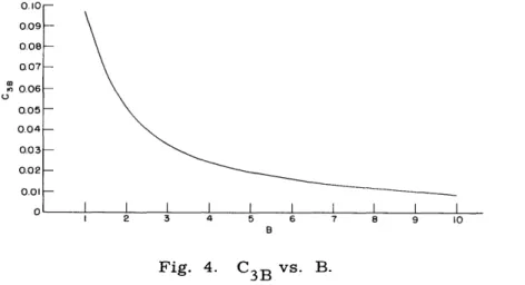
+ Re[Y(f)] (47)If the transmission network is bandlimited, the approximation error, C3, can be con-sidered as the sum of two components - one from bandlimiting and one that results from inaccuracy of approximation within the band. These components are called C3B and C3 , respectively.
If L(f) = 0 for frequencies that are such that If > B, and if d(t) is given by Eq. 44, with d = 1 and = 1, then
sin Trf df = 2 sin2TB J
C3B = 2 f2d f T I
The quantity C3B is plotted as a function of B
The question then arises: How well can
0.10 0.09 0.08 007 n 0.06 0 0.05 0.04 0.03 0.02 0.01 0 P OO sin u dul 2rB u (48) 0.1 in Fig. 4. For B > 1, we have C3B=X-.
r(t) represent d(t) when r(t) must be
I I I I I I I I I I
I 2 3 4 5 6 7 8 9 10
Fig. 4. C3B vs. B.
bandlimited? Let us assume that R(f) matches D(f) is zero elsewhere. Let r(t) under these conditions follows:
exactly within the band (-B, B) and be called r (t). We obtain r (t) as
r* (t-bT) =
f
sinf fcos ft df r (t-bT) = 7-f cos 2ft dfBf
d *
dt r (t-bT) = -2 BBsin 7Tf sin Zifft df
-2 sin 2B(t-(1/2)) 2 sin 2rB(t+(1/2)) 2r(t-( 1/2)) 2rr(t+( 1/2)) d r (t) dt = 1 -oo .'
I:
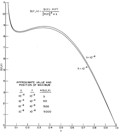
eTS 1- 1/ ) 2wB(t+(1/2)) sin x dx _- S / xIn Fig. 5, r*(t) is shown with d(t) for t > bT and B = 1.
One property of r (t), for B = 1, is that the envelope of r (t) drops off faster than (0. 056/t2) for It-bT| > 1. Thus, if we receive pulses shaped like r (t) once each second, if their separate peak values are ±1. 2, and if a sample is taken when each separate peak occurs, then the maximum possible interpulse interference is less than
00 2
2 0.- 06= (0
12)
0.2
(50)n=1 n
In this example we are signaling at one-half of the Nyquist rate. If we signal at the Nyquist rate, the maximum interpulse interference is approximately equal to the peak value of the largest single receivedpulse.
The advantages of using digital message values become apparent from the preceding
, 5 1.1 0.9 0.8 0.7 0.6 0.5 0.4 0.3 0.2 0.1 -0.1 . r(t) CASE A x r(t) - d(t) x x x x x x2
Fig. 5. Graphs of r (t), d(t), and r(t) case A.
r (t-bT) = (49) x I 5 x I x x x -0.2- v. L_
example. If we choose 4 input message values in such a way that an individual output 1 1
pulse has peak value +1, +-, -- , or -1, and if we replace each sample of the received waveform by the nearest of these values, the resulting sequence will be ideal. That is, each element will be a fixed constant multiplied by an input message value. This is because the interpulse interference is again bounded by 0. 2 and hence is never large enough to cause an error. Thus, by restricting our message values to a finite, discrete set we are able to transmit them without error through the idealized link of Fig. 2.
In the discussion of the preceding paragraphs we assumed ideal sampling instants. If the sampling instants drift more than one-fourth of the time T between messages, then, as shown by the plot of r (t) of Fig. 5, the maximum interpulse interference is at least doubled. This means that a smaller number of messages is required to obtain per-fect transmission. Of course, if the bandwidth B were increased, all other factors
*
remaining the same, then r (t) becomes flatter near the ideal sampling instant and thus is less susceptible to the effects of jitter.
10 . [H(f)] +
9-
7-APPROXIMATE VALUE AND POSITION OF MAXIMUM X3 f S(f,X) 10-2 10-2 5 10-4 10-4 50 2-- -10-6 10-6 500 10-8 10-8 5000 O 0.1 0.2 0.3 04 0.5 0.6 07 0.8 0.9 1.0 f
Fig. 6. Input pulse spectrum for two values of X.
An interesting example of the use of Eq. 46 occurs when the transfer function L(f) has a zero within the band of frequencies to be used. We assume that Y(f) = 1 and that d(t) is given by Eq. 44. We compare two cases. For case A,
IL(f) I = f I 1/2 exp(-10 f 1/2) Ifl <1 (51) For case B
IL(f)I = exp(-lOlfl
/2)
Ifl < 1 (52)In both cases L(f) is zero outside the band.
For case B the inband error can be made negligibly small. For example, if = 10 4, then r(t) for case B cannot be distinguished from the optimum bandlimited pulse, r (t), plotted in Fig. 5. For comparison, r(t), for case A and = 10 , is also plotted in Fig. 5. Note that the latter function is shifted slightly downward, because the average output of network A must be zero. The input pulse spectrum is plotted for case A and two values of X in Fig. 6.
III. LOW ERROR PROBABILITY PERFORMANCE CRITERION 3. 1 Introduction
Let us now discuss a criterion by which we can compare synchronous digital pulse links of the form depicted in Fig. 3. The adjective "digital" is intended to imply that only a finite, discrete set of amplitudes is possible for the transmitted pulses. This allows us to quantize the samples of the received waveform, and our messages can then be transmitted without errors if noise and interpulse interference are not too great.
Using our criterion, we shall optimize the performance of our link model by proper choice of the input pulse shape and linear filtering network (cf. Fig. 3). Thus we shall emphasize problems in the design of digital links, although we shall find that our results apply in other cases.
Another feature that distinguishes Section III from Section II is that for much of Section III we assume knowledge of the power density spectrum of noise that is added in the transmission network (cf. Fig. 3). This will enable us to combat the effects of this noise by means other than increasing signal power.
3. 2 Low Error Probability Criterion for a Noiseless Link
We shall now develop a criterion for judging digital links of the form shown in Fig. 2. Our particular assumptions about this model are:
1. The link is digital. That is, each element of the message sequence {an} is assumed to be selected from the same set, A, of M real numbers, (A1, A2 ... AM). As discussed
in section 2.1, each element of {an} corresponds to one transmitted message.
2. We attempt to recover the transmitted sequence {an} by quantizing the sequence of samples, {Sn}, rather than by dividing each element of {n} by r(bT), as discussed in section 2. 2. As before, the ideal sampler output is the sequence {anr(bT)}. Since
our link is now digital, each element of this sequence is a member of the set (A1r(bT), A2 r(bT),... , AMr(bT)).
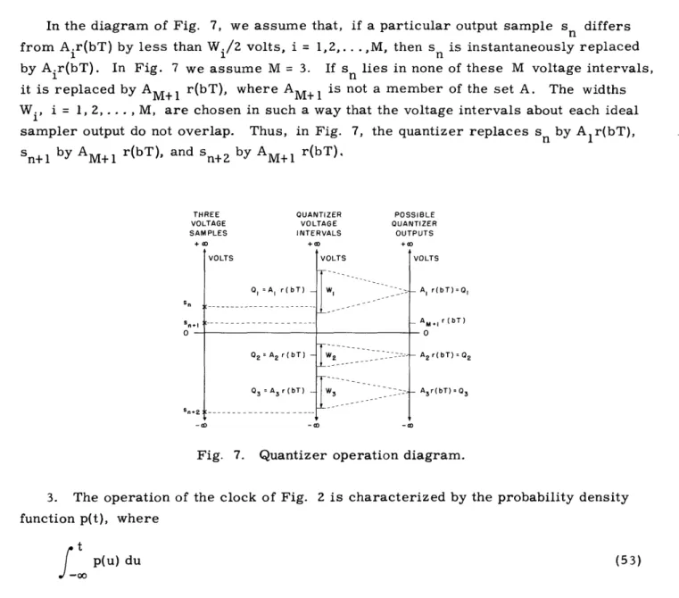
In the diagram of Fig. 7, we assume that, if a particular output sample sn differs from Air(bT) by less than Wi/2 volts, i = 1,2,.. .,M, then sn is instantaneously replaced by Air(bT). In Fig. 7 we assume M = 3. If sn lies in none of these M voltage intervals, it is replaced by AM+1 r(bT), where AM+ is not a member of the set A. The widths Wi, i = 1, 2, .. ., M, are chosen in such a way that the voltage intervals about each ideal sampler output do not overlap. Thus, in Fig. 7, the quantizer replaces sn by Alr(bT), Sn+1 by AM+1 r(bT), and n+2 by AM+l r(bT).
THREE QUANTIZER POSSIBLE
VOLTAGE VOLTAGE QUANTIZER
SAMPLES INTERVALS OUTPUTS
D +ao +ao Sn $nvl 0 -Sn.2 VOLTS 0Q =AI r(bT) _ Q2 =A2r(bT) -Q3 = A3r(bT) - ...-VOLTS _ __ ___ VOLTS -A r(bT)=OI -AM., r(bT) -O -0 - A2r(bT)=Q2 - A3r(bT)=Q3
Fig. 7. Quantizer operation diagram.
3. The operation of the clock of Fig. 2 is characterized by the probability density function p(t), where
t
_t
p(u) du (53)is the probability that the actual sampling instant that corresponds to the ideal sampling instant t = 0 occurs before time t. The correspondence between the actual and ideal sampling instants was defined in section 2. 1. The probability density p(t) is assumed to be nonzero only during the time interval (-T/2, T/2). We also assume that the proba-bility density function for the sampling instant that corresponds to the ideal sampling instant t = jT is p(t-jT), j = 0, +1, ±2 .. Each sampling instant is statistically inde-pendent of all others. Physically, we assume that any drifting of the sampling instants in either time direction is prevented, for example, by transmitting special retiming pulses to resynchronize the clock. In this case, thermal noise in the clock could cause our statistically independent jitter.
We say that our link operates perfectly if the actual sequence of quantizer outputs
{qn)
is the same as our ideal sampler output sequence {anr(bT)}. Note that our definition of the quantizer operation (cf. assumption 2 and Fig. 7), and the fact that our link isdigital (cf. assumption 1), imply that the sequence {anr(bT)} would pass through the quantizer unaffected. The probability that qn is not equal to anr(bT) for a particular integer n, say n = 0, is called the error probability. If the ensemble of message sequences [{an}] is ergodic, the error probability is independent of n.
If it is equally important that all of our M messages be transmitted correctly, low error probability is a natural criterion for good digital link performance. This is because each incorrect message receives equal weight. But there are two reasons for not using the error probability directly as a criterion. First, calculation of the error probability requires detailed a priori knowledge that would not normally be available to the system designer. For example, it is necessary to know the probability of occurrence of each message. Second, direct application of the error probability in our design prob-lems is mathematically difficult.
Our criterion for low error probability is that an upper bound, U, to the error prob-ability must be small. To derive U we first note that an error occurs whenever
W.
IQi-fs(ts)
> 21 (54)where f(ts) is the voltage amplitude of the sampled waveform (cf. Fig. 2) at a sampling instant ts. The quantities Wi and Qi are the width and center of the voltage interval within which f(ts) must lie if the correct message is to be received (cf. Fig. 7). Since there are M possible messages, the integer i may be 1, 2,...,M-1, or M.
The error probability, PE' can be written
PE Pr
L
Yi(ts) I>-
p'(i) (55)i=
where Pr [I yi(ts) I>(Wi/2)] is the probability that I Yi(ts) I exceeds (Wi/2); p'(i) is the probability of occurrence of the transmitted message value Ai, i = 1, 2, ... , M; and Yi(ts) = fd(ts) - fs(ts) is the difference between a desired waveform, fd(t), and the actual sampled waveform, fs(t), at time t = ts, given that the correct quantizer output at t = ts is Qi'
The desired waveform at the sampler input, fd(t), is defined by 00
fd(t) =
>
an d(t-nT) (56)n=-oo
where {an) is the input message sequence and
{d for p(t-bT) > 0
d(t) = (57)
L
0 otherwise The real number d is such thatAs in Section II we assume that the approximate time delay of the link is bT seconds, where b is a positive integer. We recall that p(t-bT) is the probability density function
for the sampling instant that occurs during the time interval (bT- 2T, bT+ I T). Thus, at all possible sampling instants, the desired waveform lies in the center of the correct voltage quantization interval. The only possible values for fd(t) are zero and the center voltages Qi', i = 1, 2, ... ., M.
We now apply Tchebycheff's theorem to each term in the summation of Eq. 55 to obtain our upper bound, U. Tchebycheff's theorem can be stated as follows (18):
If z is a random variable with mean m and variance -r2 and if P is the probability that I z-mI exceeds k, then P does not exceed ar2/(kor) 2 .
Thus, if mi, the mean of Yi(tS), is zero, we can write
Pr Yi(ts), I ~< w2 (59)
1
by Tchebycheff's theorem, for i = 1, 2, .. , M. The quantity ai is the variance of the random variable Yi(ts). We can now use Eqs. 55 and 59 to obtain
M 2
40i p'(i)
PE - 2U= (60)
i=l i
If we assume that the quantization intervals are of equal width, that is, W1 = W2 . = WM = W, then Eq. 60 can be written in the simpler form
4- 2 U z (61) W where 2 M 2 0. = 1
p'(i)
(62) i=l3. 3 A More Explicit Expression for the Low Error Probability Criterion
In obtaining a more explicit expression for the low error probability criterion we make the same assumptions that we made in section 3. 2. In addition, we assume that the ergodic message sequence {an} has correlation function m (n) and that
E[an] = m(OO) = 0 (63)
where E[
]
denotes the ensemble average of [ ]. We also assume thatW 1 W 2 = W M = W (64)
If we are given two possible input pulse shapes s1(t) and s2(t), we shall say that sl(t) is better than s2(t) if
U(s (t)) U(s2(t)) (65)
where U(s(t)) is the value of U when the input pulse shape s(t) is used. An optimum input pulse shape is one for which U is a minimum.
We recall that the validity of Eqs. 59, 60, and 61 depends on the conditional means, mi, i = 1, 2 ... , M, being zero. However, we shall now show that in the case of Eq. 61 we need only require that
M
m = E[fd(ts)-fs(ts)] = E miP'(i) = 0 (66)
i=l
This follows from the fact that the error probability may be written
P- Pr
[Iy(t
)>i 2] (67)if the quantizer voltage intervals have equal width W. The quantity y(ts) is the difference fd(ts) - f(ts). If m = 0, Tchebycheff's theorem can be applied directly to Eq. 67 to give Eq. 61. Physically, Eq. 66 requires that the expected value of each sample of the actual
received waveform be equal to the value of the desired waveform at that instant. We shall now write m explicitly in order to obtain sufficient conditions for m = 0. Using the definitions of fd(t) and fs(t) (cf. Fig. 2 and Eq. 56), we obtain
00oo
E[fd(t)-fs(t)] = E E[an](d(t-nT)-r(t-nT)) (68)
n=-oo
Thus, if, as we have assumed, E[an] = 0, then
m = E[fd(ts)-fs(ts)] = 0 (69)
Before we can minimize U by varying s(t) it is necessary to rewrite U in such a way 2
that its dependence on s(t) becomes more apparent. We first calculate 2
00oo y(t) = fd(t)- f(t) = E an(d(t-nT)-r(t-nT)) (70) n=-oo y2(t) =
Z
aiaj(d(t-iT)-r(t-iT))(d(t-jT)-r(t-jT)) (71) i=-oo j -oo E[y2(t)]=e.
(i-j)(d(t-iT)-r(t-iT))(d(t-jT)-r(t-jT)) i=-oo j=-oo = .(m
(k)(d(t-iT)-r(t-iT))(d(t+kT-iT)-r(t+kT-iT)) (72) i=-oo k=-o m 19We note that the ensemble average E[y2(t)] is not, in general, independent of t. That is, the ensemble [y(t)] is nonstationary. This type of nonstationary random process has been discussed by W. R. Bennett (19).
To obtain E[y2(ts)] we must also average over the possible instants at which any one sample could be taken. We assume that (n-(1/2)) T < t < (n+(1/2)) T, but we shall find
s
that E[y(ts)] is independent of n, n = 0,l,i±2,.... Since m = 0,
2 E 2(t1 (n+(1/2))T 2
or EIn-(1/2))T J p(t-nT) E[y (t)] dt (73)
Substitution of Eq. 72 and a change of variable u = t - iT gives
' = E (n+(/2))T p(u+iT-nT) m(k)[d(u+kT)r(u+kT)][d(u)-r(u+kT)][d(u)-r(u)] du
i=-oo j n-( 1/2))T-iT k=-oo
(74) Performing the summation on i, we obtain
r
=
~ p(u+iT) . qm(k)[d(u+kT)-r(u+kT)][d(u)-r(u) ] du (75)-oo i=-oo k=-oo
For the case of uncorrelated messages
~m(k) = 0 k = ±1,±2... (76)
and Eq. 75 becomes
e2 = (0) puiT)[d(u)-r(u)]2) dt (77)
00 i=-00
For this case we can obtain U by substituting Eq. 77 in Eq. 61.
U= 02
J)
Z p(u+iT)[d(u)-r(u)]2) dt (78)W -o00 i=-o00
We recall that r(t) is the response of the transmission network of Fig. 2 to an input pulse s(t); d(t) is an ideal received pulse shape that is defined in Eq. 57; p(t+iT) is the probability density function for the sampling instant that occurs in the time interval
i-2
(-+
)
T); m(k), k = 0, 1, 2,..., is the discrete correlation function of the ensemble of message sequences [{an}]; and W is the voltage width of each of the M voltage quantization intervals (cf. Fig. 7).We have shown that U is a suitable criterion with which to judge our link, because U is an upper bound to the error probability. Aside from this, U also satisfies more intuitive requirements for a good criterion.
Since there is no noise in our link, errors are caused only by interpulse interference,
and U of Eq. 78 is very similar to the low interpulse interference criterion, C3, of Eq. 45. Both U and C3 are least squares criteria, but the integrand of U in Eq. 78
is weighted by the sum of the probability density functions p(t+iT), i = 0, ±1, ±2,.... This weighting factor restricts the integration to possible sampling instants and gives more importance to probable sampling instants. This makes U a more satisfying criterion than C3, because C3 equally requires r(t) to be small, irrespective of the likelihood of a sample, when d(t) is zero. The choice of r(t) according to either cri-terion tends to keep r(t) large at the correct sampling instant, that is, the one closest to t = bT. However, the use of U again stresses the importance of the more probable sampling instants.
Let us now write the expression for U of Eq. 61 in the time and frequency domains for the case of correlated messages. Substituting Eq. 75 into Eq. 61 gives
U 2
(
X p(u+iT)[d(u)-r(u)] E pm(k) [d(u+kT)-r(u+kT)] du (79)W 01 i=-oo k=-oo
We now note that the Fourier transform of
00oo
fl(u) = [d(u)-r(u)] p(u+iT) (80)
i=-00oo
is
F 1(f) T Xo ( Y [ () - T )] (81)
n=-oo
where P(f), D(f), S(f), and L(f) are the Fourier transforms of p(t), d(t), s(t), and f(t), respectively. For example,
r0
S(f) = s(t) exp(-j2rft) dt (82)
-o0
In writing Eq. 81 we use the fact that R(f) = S(f) L(f) (cf. Fig. 2). The Fourier transform of
00 f2(u) =
>
,m(k)[d(u+kT)-r(u+kT)] (83) k=-oo is F2(f= m(f)[D(f)S(f)L(f)] (84) where 00 00 m(f) = m(k) exp(j2rrkTf)= k ,m(k) cos 2TkTf (85) k=-oo k=-ooIn writing Eq. 85 we use the fact that m(k) is an even function. Thus, by use of Parceval's theorem, we obtain
Fl(f) F2(f) df
n--oo ( (D _ S (f_ T L f(f)[D )] ( f )- S( f)L (f)) df
(86)
where the asterisk denotes a complex conjugate.
3. 4 A Necessary Condition for an Optimum Transmitted Pulse Shape
We shall now obtain an equation that must be satisfied if U is to be minimized by proper choice of S(f). Using standard techniques of the calculus of variations we assume that there exists a signal pulse spectrum, S(f), that minimizes U (ref. 16). Such spectra
exist. For example, if there are no constraints on S(f), we can choose S(f) in such a way that S(f) L(f) = D(f). In this case, U = 0, and this is as small as U can be.
We assume that S(f) is constrained to be nonzero only for some set of frequencies, F. It is convenient, but not necessary, to think of F as a base band of frequencies (-B, B). Physically, this constraint might result from (a) an artificial frequency restriction, such
as the allotment of a band of frequencies to one channel of a frequency division system, or (b) a natural restriction, such as excessive transmission attenuation outside a certain band of frequencies or practical difficulties in generating pulses with appreciable energy
at arbitrarily high frequencies.
We assume that S(f) is a spectrum that minimizes U and we replace S(f) of Eq. 86 by S(f) + ap(f), where a is a real parameter, and f3(f) is the Fourier transform of a real function. The function P(f) is zero if f is not in the set F. Any possible signal pulse spectrum can be represented in the form S(f) + ap(f). Since S(f) is an optimum spectrum, U is a minimum if a = 0. Thus, we require that
au
a a = 0
I
00ooT
n=-oo+ (T n-oo P(T)[(f T-)L(f T)*(f[D*(f)- S*(f)L*(f)]) df= O
00 n= 0
(87)
This derivative is calculated from Eq. 86. We may rewrite Eq. 87 by making of variable u = (n/T) - f in the second integral. We also use the fact that P(-f) This follows from our definition of Mf). We then have
au aa a=O
the change = (f).
- (p*(f) (f) L*(f) P(f-)-S (f- T(f- ) df
T
-#:k\
13(u) L (u) P (T)[D ( -S(u- -S u- u- (- du= 0 (88)U 4 006
4 00
W2 oocoT
In writing the second integral in Eq. 88 we have used the fact from Fourier theory that S(-f) = S(f), L(-f) = L (f), and D(-f) = D*(f). If we can show that
oo oo ID(f) O" p n -,) nH \ C P · , ) H(f_ n D.(f_ X "Y)T -T
X
T
n=-oo n=-oo where H(f) = D(f)- S(f) L(f) (89) (90) then, by substitution of Eq. 89 into Eq. 88, we obtain2 p (f) 1*%(f) L*(f) E
J0
n=-ooTI p(n)H(f-,-)df = 0 (91)
The validity of Eq. 89 is shown by transforming its right-hand side. By using the definition of m(f) in Eq. 85, the right-hand side of Eq. 89 is
(92)
Using the fact that cos 2kT(f- T) = cos 2kTf and interchanging the order of summation gives
(93)
00 ( )
n=-oo
Eq. 85 shows that *m(f) = m(f). Thus, expression 93 is equivalent to the left-hand side of Eq. 89. Hence, Eqs. 89 and 91 are valid.
Since P*(f) is zero for all frequencies that are not in the set F and * (f) can be non-zero at any or all of the frequencies in F, a necessary condition for Eq. 91 to hold is that
T P(n) H(f- ) =
TT T~I- 0 for all f in F (94)Using Eq. 90 and the fact that '%(f) = m(f), we may rewrite Eq. 94 as
0o cm(f) L*(f) 0 n=-oo n-oo n=-oo T P() S(f T) L(f-T) = (f) L*(f)
Y
T
for all f in F The term noo n=-o 23 4m(f) L(f) n=-oo (95) n00~T=00
1 P (-,n D (f- n IP (-, ) Df n) Y'T T00
can be recognized as the Fourier transform of d(t) _ p(t+jT). From the definition
j=-00
of p(t) (Eq. 53 et seq.) and d(t) (Eq. 57) it follows that
00oo
d(t) p(t-jT) = dp(t-bT) (96)
J=-00
Thus, Eq. 95 may be written as
1)m(f) L *(f) E_ T P(n) S(f ) L( )
= d m(f) L (f) P(f) exp(-jTbTf) for all f in F (97)
Therefore, if s(t) is an optimum transmitted pulse shape, then its Fourier transform S(f), must satisfy Eq. 97. We now wish to give some interpretation of Eq. 97.
For all frequencies that are such that
m(f) L (f) 0 (98)
Eq. 97 is equivalent to
T P )S(f-) L(fT = dP(f) exp(-j2rrbTf) for all f in F' (99) n=-oo
where F' is the set of frequencies that are in the set F and that satisfy condition 98. If F' includes all frequencies, (-oo, oo), then the result of taking the Fourier transform of both sides of Eq. 99 is
00oo
r(t) p(t-nT) = dp(t-bT) (100)
n=-oo
Thus, the received pulse shape r(t) should be equal to d(t) when . p(t-nT) is n=-oo
nonzero, and r(t) is undefined for other values of t. This agrees with our discussion at the beginning of this section.
In this section we have shown that, if F, and hence F', do not include all fre-quencies, then Eq. 97, and Eq. 99, must be satisfied. That is, at every frequency at which we are allowed to transmit power, the Fourier transform of the left-hand side of Eq. 100 should equal the Fourier transform of the right-hand side. The
left-00
hand side of Eq. 100 can be interpreted as a periodic function, X p(t-nT), that has
n=-oo
been amplitude-modulated by a pulse, r(t). Equation 97 was derived previously by the writer in a less direct manner (20).
3. 5 Optimum Pulse Shapes for a Noiseless Link
We shall now solve Eq. 99 for R(f) = S(f) L(f). This is equivalent to solving for S(f), because
(a) If f is not in the set F, defined at the beginning of section 3. 4, then R(f) = S(f) = 0.
This follows from the definition of F. R(f)
(b) If f is in the set F', defined in connection with Eq. 99, then S(f) = , because L(f)
L(f) is not zero. A special case occurs if f is in F, but is not in F'. It can then happen that L(f) is zero, but R(f) is not zero, and thus S(f) will be infinite. This special case,
that is, Eq. 99 not equivalent to Eq. 97, will be taken up in section 3. 7. We wish to solve the equation
I P(n) R(f- ) = dP(f) exp(-jZrrbTf) for all f in F' (101) n=-oo
This equation is to be solved for R(f). We first note that, for the case in which F' is contained in an open interval (-B, B) and 1/T > 2B, Eq. 101 reduces to
R(f) = dTP(f) exp(-j27rbTf) for all f in F' (102)
because here F = F'; R(f) is zero outside F; and (/T) is chosen large enough so that none of the terms R (f- T) is nonzero in F'. This is best visualized by considering the special case F' = (-B, B).
For example, let F = F' be the open interval (-B cps, B cps) and let p(t) be a unit impulse that occurs at t = 0. That is, we assume dete.rministic, periodic sampling. If 1/T > 2B, Eq. 102 and the definition of F imply that
rdT
exp(-j2ibTf) for If < B R(f) = (103) o0 otherwise Thus 2BdT sin 2rrB(t-bT) r(t) = (104) 2w B(t-bT)We note that, if 1/T = 2B, then r(bT) = d. We recall that d is the desired received pulse amplitude at its sampling instant. As T decreases, r(bT) decreases. This might be expected from the fact that, if we receive pulses like that of Eq. 104 faster than 2B per second, the pulses will overlap. The results of this example, that is, Eqs. 103 and
104, in the special case 1/T = 2B agree with those obtained by Nyquist (21).
As another example, let us again consider the assumptions of the previous example, except that we now assume 1/T = B. In this case Eq. 101 becomes
R(f+B) + R(f) + R(f-B) = dT exp(-j2rrbTf) for IfI < B (105)
Unlike the previous example, where the solution was unique, we now have many possible
solutions. One solution is R(f) dT exp(-j2rbTf) for If < B (106) otherwise Another solution is 1dT exp(-j2irbTf) for If < B R(f) = (107) 0 otherwise
The received pulse shape that corresponds to Eq. 106 is
d[sin Z2B(t-bT)]2
r(t) = (108)
[2TB(t-bT)]
This example seems to indicate that if we are willing to signal slower than the Nyquist rate 1/T = 2B, then we gain more freedom in the choice of our received pulseshape. However, we shall see that this conclusion applies only to deterministic, periodic sampling.
We shall now solve Eq. 101 by rewriting it as a set of simultaneous, linear equa-tions. We assume that the probability density function p(t) is positive over some time interval of positive extent. That is, we shall no longer consider p(t) to be an impulse. The set F', over which R(f) is nonzero, is assumed to lie within some interval (-B, B).
Given any particular frequency f in F' we let {xj} be the set of ordered (1/T) trans-lates of f that lie in (-B, B). That is,
(1) x. is in (-B, B) 1 for i = 1, 2,..., N' (2) = + T for i = 2, 3 ... ,N'
(3) x. = f for some j, j = 1, 2, ... , N'
and N' is the number of elements of the set f+ n , n = 0,±l,±2,. , that lie in (-B, B).
The integer N' must be finite, because B is assumed finite. For f = x we can write Eq. 101 as
N' (n-j\
Z
P R(xn) = dTP(x.) exp(-j2rbTx.) (109)n= 1
If we now let j = 1, 2, ... , N', we obtain a set of N' simultaneous linear equations. If
N is the number of elements in the set {xj} that belong to the set F', then only N of these N' equations need hold, because Eq. 101 must only be satisfied for f in F'. Now let {fj}, j = 1, 2, ... . N, be the elements of {xj} that are in F', and let f > f2 > ... > fN'
Of the N' unknowns in the remaining N equations, only R(f1), R(f2),. .. ., R(fN) are not known to be zero. This follows from our assumption in this section that F' = F and from our definition that R(f) = 0 for values of f that are not in F.
If F' is the interval (-B, B), equations is
DN =
P(O)
P(O)
then N = N', and the determinant of our set of linear
... p(N-1
... p(N-2)
p(N+l) p(-N+2) p(-N+3
P(O)
For other choices of F' some of the columns and their corresponding rows do not appear in DN.
If DN is not zero, we can solve our set of equations by Cramer's rule (22). The unique solution for f = f. is then
J P(fl)D( ,) + P(f2)D(2,) +... + P(fN) D(NN 'j )dT exp(-j2rrbTxj) R(fj) = DN 0 otherwise for f. in F' J
where Dn(i' is the cofactor of the (i, j) element of DN.
We shall now prove the validity of Eq. 111 by demonstrating that the determinant DN is always positive. We note from Fourier theory that, because p(t) is real, its Fourier transform, P(f), has the property that P *(f) = P(-f). This implies that the matrix cor-responding to DN is Hermitian. It then follows that DN is positive if its associated quadratic form
N' N'
i=l k=l
AiAk (1T) (112)
is positive definite (23). If our set F' does not cover the whole band (-B, B), then some of the coefficients A are zero. We wish to show that expression 112 is positive, unless A A = AN 0.
Schetzen has shown that this expression is non-negative definite (24). We shall extend his argument to obtain our result. We first rewrite expression 112.
N' N' k-i T/2 i=l k=l T/ 2 N' N' i=l k=l
iTT/2
N' -T/2 T/2 p(t) k= 1 AiAkP(t) exp(-j2k)t) dt Ak exp(-j2rr kt) dt 27 (110) (111) (113)N'
We now note that, unless A1 = A2 =...AN, *t = 0,
Z
Ak exp -j2w can be zero fork=l N'
at most N' values of t. This follows from the fact that the polynomial Akzk can k=l
have only N' roots, unless A = A2 = = AN, = 0. Since we assumed that p(t) is
positive over some subinterval of (-(T/2), (T/2)), it follows that the last integral in Eq. 113 will be positive, unless A1 = A2 = = AN, = . This proves that DN
is positive and hence that, under our assumptions, a unique solution to Eq. 101 always exists and is given by Eq. 111.
We note that if p(t) is an impulse our proof does not apply because a zero of N'
Ak exp(-j2 T t) can coincide with and cancel the impulse. This agrees with our k=l
second example, given earlier in this section, in which the solution of Eq. 101 was not unique and p(t) was assumed to be an impulse.
We shall now work out an example to demonstrate what computations must be made when we apply Eq. 111. The set F' is assumed to be the open interval (-B,B), 1/T = B, and
2- for ItI <T p(t) =T 4 0 otherwise Henc e, sin rw(T/2) f P(f) = 7(T/2) f (114) (115)
If we choose f = x. in (-B, B) but not f+ 7, only f and f (1/T) can lie because ±B do not lie within (-B, B)
P(O)
P(O)
D1 = P(O) = 1
equal to zero, then N = N' = 2. That is, in the set in (-B, B) because 1/T = B. If f = 0, then N = N' = 1,
(116) p()p() = 1 4
(117)
Application of formula 111 now yields
sin [(T/2)f] 2 sin [(T/2)(f+I/T)]
rr(T/2) f rw(T/2)(f+l/T) - 4/2r dT exp(-j2rrbTf) dT f = 0 sin [r(T/2)f] 2 sin [rr(T/2)(f-1/T)] ___T_2_ Tf-- dT exp(-j2wbTf) ~(T/2) f w ~(T/2)(f- 1/T) 1 - 4/rr 28 R(f) = -B <f < 0 (118) 0<f<B
It is important to note that the form of Eq. 111- in particular, the order of the determinant DN - depends strongly on the rate of signaling, (/T), because this rate controls the number of elements of {f+T} that lie in F'. If F' is a base band of fre-quencies, (-B, B), and if we signal faster than the Nyquist rate 2B, then Eq. 111 can be written in the simpler form of Eq. 102. As we reduce our signaling rate, R(f), for any particular f, becomes a linear combination of many values of P(f).
3. 6 Low Error Probability Criterion for a Noisy Link
In this section we assume that noise added during the transmission of our signal can no longer be neglected. This might come about because an excessive amount of signal power is required to overcome the noise, or because we know the power density spec-trum of the noise and wish to use this knowledge to reduce the effects of the noise. We
shall consider the synchronous link model of Fig. 8.
With the exception of the gaussian noise generator, the dc voltage source, and the decoder, all of the blocks of this model have been discussed in connection with Figs. 1,2,
and 3. We recall (from sec. 2. 1) that the message source produces a periodic train of area modulated impulses, m(t), where
00
m(t) = E an u0(t-nT) (119)
n=-oo
and uo(t) is a unit impulse that occurs at t = 0. Each element an of the message sequence{an}is chosen from a finite set A. That is, the link is assumed to be digital. The real numbers, (A1, A2 .. ., AM), that constitute A, are assumed to be in one-to-one correspondence with M possible transmitted messages. The message probabilities are such that Ai occurs at any particular place in a message sequence with probability p'(i), i = 1, 2, ... , M, and the correlation function of the message sequence ensemble
[{an}] is m(n).
The linear, pulse-forming network has output response s(t) to a unit impulse input. The Fourier transform of s(t) is denoted by S(f). The input to the transmission network is then
00
fI(t) = E an s(t-nT) (120)
n=-oo
In a real link the individual input pulses might be transmitted by triggering some non-linear device every T seconds. However, an input pulse train like fI(t) can always be represented as the response of a linear network to an impulse train, and this latter representation is convenient conceptually and mathematically.
The linear transmission network has output response (t) to a unit impulse input. The Fourier transform of (t) - that is, the network transfer function - is denoted by L(f). The noise waveform n(t) is added to the output of the transmission network to represent the effects of noise in the transmission network. The random waveform n(t)
S(f) s(t) L(f)
fo (t)
P (M) - AM
PROBABILITY DENSITY FOR SAMPLING INSTANTS
p(t) -T T 2T 3T QUANTIZER POSSIBLE VOLTAGE DECODER INTERVALS OUTPUTS 03 WI A3 2V2 O I _- .. ... A/.. A
(DEPICTED FOR M3) M.I
Fig. 8. Synchronous digital link model.
is assumed to be a member of a noise ensemble [n(t)] that has correlation function n(r) and power density spectrum n(f).
The resulting waveform is the input for a linear, pulse-shaping amplifier that has output response a(t) to a unit impulse input. The Fourier transform of a(t) is A(f). White,
2
gaussian noise, n(t), with mean iI 11 and variance an and dc voltage V are added to then 1~~~~~~~
output of the amplifier. of the dc voltage will be
The waveform at the
Noise in the amplifier is represented by nl(t). The purpose discussed later.
input to the sampler is called fs(t), and
00 /00 fs(t) =
Z
an r(t-nT) + n(t) + V + n=-oo -oo n(x) a(t-x) dx where oo -oo -oo s(x)(u-x) dx] a(t-u) du (122)The linearity of the transmission network and the amplifier enables us to interpret each term of fs(t) as the result of a separate cause. The first term is the result of passing the input waveform, fI(t), through the transmission network and amplifier; the next two
terms are the direct result of their addition to the amplifier output; and the fourth term is the result of passing noise waveform n(t) through the amplifier.
( 121)
4)" ( ) 0 (') P (f) pP M
la
f, ( ) =C ., s t- nT
The sampler instantaneously samples its input whenever it receives an impulse from the clock. We assume, as before, that there exists a small time interval about each time instant jT, j = 0, ±1, +2.... These time intervals have the property that one and only one sampling instant occurs within each interval. The probability density function for the sampling instant that occurs in the jth interval is p(t-jT), j = 0, ±1, +2... . See Fig. 8.
We assume that the quantizer operates as discussed in connection with Fig. 7. That is, the sequence of sampler outputs, {sn}, is sorted sequentially into M voltage intervals, each of which corresponds to a distinct member of the message set A. The decoder instantaneously replaces each sample by an element of A according to this correspond-ence. If a voltage sample happens to lie in none of the M intervals, the decoder replaces it by the number AM+l, where AM+1 is not an element of the set A. The operation of the quantizer and decoder is depicted in Fig. 8, where it is assumed that M = 3, and the M voltage intervals are contiguous and lie within a voltage interval of width 2v2 volts.
We say that the link performs perfectly if the sequence of decoder outputs is the same as the message sequence, {an}, except for a finite time delay. The probability that these sequences will differ in any one place is called the error probability. The discussion in section 3. 2 on the use of an upper bound to the error probability as a cri-terion for link performance and our reasons for not using the error probability directly apply to our present case as well.
We also note that the necessary and sufficient condition for an error given in Eq. 54 is valid for our noisy model. Also, the steps that lead from Eq. 54 to Eqs. 60 and 61 hold because they did not depend on the fact that our link was noiseless. In using Eqs. 54-62 in connection with our model of Fig. 8 we need only use the fact that fs(t) is now defined by Eq. 121.
Thus, from Eqs. 60 and 61, our criterion for good link performance in our model of Fig. 8 is that U be small, where
M 42 p'(i)
U= Z 2 (123)
i=l W
in the general case, and 42
U= W2 (124)
W
in the case of equally wide quantization intervals.
3. 7 Necessary Conditions for Optimum Pulse Shapes in a Noisy Link
We shall now use the methods developed in section 3. 4 to minimize U by varying the input pulse spectrum, S(f), and the amplifier transfer function, A(f).