HAL Id: tel-01358567
https://tel.archives-ouvertes.fr/tel-01358567
Submitted on 1 Sep 2016HAL is a multi-disciplinary open access archive for the deposit and dissemination of sci-entific research documents, whether they are pub-lished or not. The documents may come from teaching and research institutions in France or abroad, or from public or private research centers.
L’archive ouverte pluridisciplinaire HAL, est destinée au dépôt et à la diffusion de documents scientifiques de niveau recherche, publiés ou non, émanant des établissements d’enseignement et de recherche français ou étrangers, des laboratoires publics ou privés.
video imagery
Donatus Bapentire Angnuureng
To cite this version:
Donatus Bapentire Angnuureng. Shoreline response to multi-scale oceanic forcing from video imagery. Earth Sciences. Université de Bordeaux, 2016. English. �NNT : 2016BORD0094�. �tel-01358567�
POUR OBTENIR LE GRADE DE
DOCTEUR DE
L’UNIVERSITÉ DE BORDEAUX
ÉCOLE DOCTORALE
SPÉCIALITÉ
Physique de l’environnement
Par Donatus Bapentire Angnuureng
Shoreline response to multi-scale oceanic forcing
from video imagery
Sous la direction de : Nadia Senechal
(co-directeur : Rafael Almar)
(co-directeur : Bruno Castelle )
(co-directeur :Kwasi Appeaning Addo)
Soutenue le 06/07/2016
Membres du jury :
M. HALL Nicholas Professor Université de Toulouse Président M. ANTHONY Edward Professor CEREGE, Aix-Provence Rapporteur
M. OUILLON Sylvain Professor IRD-LEGOS Rapporteur
Résumé :
Le but de cette étude était de développer une méthodologie pour évaluer la résilience des littoraux aux évènements de tempêtes, à des échelles de temps différentes pour une plage située à une latitude moyenne (Biscarrosse, France). Un site pilote des tropiques, la plage de Jamestown (Ghana), non soumis aux tempêtes, a également été analysé. 6 ans (2007-2012) de données sur la position du trait de côte, obtenues quotidiennement par imagerie vidéo, ainsi que les prévisions hydrodynamiques (ECMWF EraInterim) ont été analysées. Le climat de vagues est dominé par les tempêtes (Hs> 5% de seuil de dépassement) et leurs fluctuations saisonnières; 75% des tempêtes se produisent en hiver, et plus de 60 tempêtes ont été identifiées au cours de la période d'étude. Une régression multiple, montre qu’alors que les intensités des tempêtes actuelle et précédente ont un rôle majeur sur l'impact de la tempête, la marée et les barres sableuses jouent un rôle majeur sur la récupération de plage. La position moyenne du trait de côte calculée sur la période de récupération post-tempête montre que la plage de Biscarrosse se reconstruit rapidement (9 jours) après un évènement isolé et que les séries de tempêtes (clusters) ont un effet cumulatif diminué. Les résultats indiquent que le récurrence individuelle des tempêtes est clé. Si l'intervalle entre deux tempêtes est faible par rapport à la période de récupération, la plage devient plus résistante aux tempêtes suivantes; par conséquent, la première tempête d’une série a un impact plus important que les suivantes. Le trait de côte répond, par ordre décroissant, aux évènements saisonniers, à la fréquence des tempête et aux d’échelle annuelle. La méthode EOF montre de bonnes capacité à séparer la dynamique « uniforme » et « non-uniforme » du littoral et décrit différentes variabilités temporelles: les échelles saisonnières et à court terme dominent, respectivement, la première EOF (2D) et le second mode (3D). Le littoral de Jamestown a été étudié comme base d’un projet pilote entre 2013-2014. Les fluctuations du niveau de l'eau jouent un rôle prédominant sur l’évolution de la position du trait de côte. Les vagues et les estimations des marées obtenues par l’exploitation d’images vidéo sont corrélées avec les données de prévisions. Cette étude pionnière montre que cette technique peut être généralisée à toute l’Afrique de l'Ouest en tenant compte des multiples diversités et de la variabilité du climat régional, à travers un réseau d'observations.
Mots clés :
Abstract :
The aim of this study was to develop a methodology to statistically assess the shoreline
resilience to storms at di
fferent time scales for a storm-dominated mid-latitude beach
(Biscarrosse, France). On a pilot base, storm-free tropical Jamestown beach (Ghana) was also
analysed. 6-years (2007-2012) of continuous video-derived shoreline data and hindcasted
hydrodynamics were analysed. Wave climate is dominated by storms (Hs>5% exceedance
limit) and their seasonal fluctuations; 75% of storms occur in winter with more than 60
identified storms during the study period. A multiple regression on 36 storms shows that
whereas current and previous storm intensity have predominant role on current storm impact,
tide and sandbar play a major role on the storm recovery. An ensemble average on
post-storm recovery period shows that Biscarrosse beach recovers rapidly (9 days) to individual
storms, and sequences of storms (clusters) have a weak cumulative effect. The results point out
that individual storm recurrence frequency is key. If the interval between two storms is low
compared to the recovery period, the beach becomes more resilient to the next storms; and the
first storm in clusters has larger impact than following ones. Shoreline responds in decreasing
order at seasonal, storm frequency and annual timescales at Biscarrosse. The EOF method
shows good skills in separating uniform and non-uniform shoreline dynamics, showing their
different temporal variability: seasonal and short-term scales dominate first EOF (2D) and
second (3D) modes, respectively.
The shoreline at Jamestown was studied on pilot base from 2013-2014. Water level channges
play a major role on shoreline changes. Waves estimates from video are in good agreement with
hindcasts. This study shows the potential of the technique, to be replicated elsewhere in West
Africa with all its diversity and regional climate variability through a coastal observation
network.
Keywords :
[EPOC, B18,
UMR CNRS 5805 EPOC - OASU
Université de Bordeaux
Site de Talence - Allée Geoffroy Saint-Hilaire
CS 50023
33615 PESSAC CEDEX
FRANCE]
4 Dedication
5 Aknowledgement
The international research stays gave me the opportunity to work with two leading laboratories in terms of coastal hydrodynamics to extreme storms and shoreline evolution as a whole. The experiences that I went through during my stays in LEGOS, Toulouse and EPOC, Bordeaux have built me not only intellectually but also personally. I am extremely grateful for having had the opportunity to meet such talented scientists and to share their expertise with me.
Many thanks to ARTS (‘Allocations de Rercherche pour une Thèse au Sud’) organisation for their immense financial support and design to strengthen research capacities in developing countries. I would also like to thank the French Embassy in Ghana for their support as ARTS. I thank also the facilitators of the Physical Oceanography and Application program in Benin; Dr. Bernard Bourles, Prof. Nick Hall and Dr. Yves du Penhoat.
I thank Dr. Nadia Senechal, my advisor, for her tireless roles as a mentor and advisor both in the field and through writing papers, administrative works and helping to advance this thesis. I would like to thank Dr. Rafael Almar co-supervisor, for first of all the creation of this thesis. His exuberance for the study and relentless passion to approach every scientific inquiry with the utmost enthusiasm influenced me to always do my best, and then try even harder to exceed my limits. Dr. Almar’s patience and hope he had in me guided me this far and this thesis would not be success without him. He has taught, challenged, and encouraged me in an apprenticeship beyond my highest expectations. I would also to like to thank Dr. Bruno Castelle, a co-supervisor, for his active and constant response to all my requests. Dr. Castelle kept me on my toes in consistence with the saying that ‘spare the rod spoil the child’. I would like to thank Dr. Kwasi Appeaning Addo, co-supervisor, for being one of the most important and influential people in my academic, educational, and personal advancements. Over the last few years, Dr. Appeaning Addo has not only been an advisor and mentor, but also as an encouraging father. I also thank Dr. Vincent Marieu for his guidance in retrieving the video data and writing of my research.
My sincere gratitude also goes to Professor Domwini Dabire Kuupole (Vice Chancellor), Dr. Denis Aheto, Dr. Anani K. Fenin of University of Cape Coast and Mr. A. K. Armah of University of Ghana for their support and helps in getting me to this level. I would also like to thank the many graduate and undergraduate students who would have helped in one way or the other with field data acquisition during this study. And lastly, my deepest gratitude to the family and friends who have given me so much love, encouragement, and support during the last three years of my thesis endeavors. Many new things are in the future and I look forward to working with all of you again.
6
TABLE OF CONTENTS
Abstract...3 Dedication ...4 Aknowledgement...5 Table of Contents...6 Glossary...10 1 Introduction...12 1.1 Motivation...14 1.2 Scientific challenge ...15 1.3 Organization of Dissertation...192 Hydro-morphodynamic coastal processes ...21
2.1 Wave dynamics in the nearshore: refraction, diffraction and breaking
...23
2.2 Beach system
...26
2.2.1 Bar-berm beach dynamics
...26
2.2.2 Wave-induced short term morphodynamics
...29
2.2.3 Tides and their control on nearshore processes
...31
2.3. Shoreline dynamics...
...34
2.3.1 Shoreline definition: a review
...34
2.3.3 Sandbar to shoreline coupling
...35
2.4. Transient and persistent effect of storms. .
...37
2.4.1 Wave climate and storminess: regional to beach scale
...37
2.4.1.a Wave climate..
...37
2.4.1.b Storms.
... ...39
2.4.2 Storm impact..
... ...41
2.4.3 Post-storm Recovery..
...42
2.5 Shoreline acquisition and prediction
...42
2.5.1 Different conventional shoreline measurement techniques ...44
2.5.2 Video monitoring: context and background ...46
2.5.2.a Video monitoring of the nearshore: 25 years of developments and use...46
7
2.5.3 Predicting shoreline evolution using models
...48
3 Study area, data and methods ...50
3.1 Description of study sites ...52
3.1.1 Environmental settings of Biscarrosse beach ...52
3.1.2 Biscarrosse beach: wave and tide forcing ...52
3.1.3 Morphology of Biscarrosse beach...54
3.1.4 Introduction to Jamestown beach...55
3.2 Hydrodynamic data at Biscarrosse...56
3.2.1 Wave data...56
3.2.2 Waterline elevation data...58
3.3 Morphological data at Biscarrosse...59
3.3.1 Pre-processing, georeferencing and rectification ...60
3.3.2 Processing of images: Biscarrosse video and merging images ...62
3.3.3 Shoreline and sandbar detection...63
3.4 Error Analysis...63
3.4.1 Inaccuracy in the shoreline location ...63
3.4.2 Inaccuracy in the sandbar location ...69
4 Statistical approach of coastal response to storms...71
4.1 Introduction... ...73
4.2. ARTICLE: Shoreline resilience to individual and sequence of storms at a meso-macrotidal barred beach (in revision, Geomorphology) ...73
4.2.1. Introduction ... ...74
4.2.2. Methods... ...77
4.2.2a Field site…... ...77
4.2.2b Video data ...78
4.2.2c Storms... ...80
4.2.3. Results... ...83
4.2.3a Characteristics of individual storms and morphological impact...83
4.2.3b Modulation of storm impact and recovery by previous events, tides and sandbar... ...87
4.2.3c Storm sequences ...88
8
4.2.4. Discussion... ………...92
4.2.4a. Role of waves and tide on storm impact...92
4.2.4b. Importance of the frequency of recurrence of storms for shoreline resilience...92
4.2.5. Conclusions………...94
5 Two and three-dimension shoreline changes at short and seasonal scales ...95
5.1 Introduction ...97
5.2 (Article): Two and three-dimensional shoreline behaviour at a meso-macrotidal barred beach (in preparation) ...97
5.2.1 Introduction ...98
5.2.2 Data and methods... ...100
5.2.2.a Study area... ...100
5.2.2.b Offshore hydrodynamic forcing ...100
5.2.2.c Video derived shoreline and sandbar...101
5.2.2.d Data processing ... ...103
5.2.3 Results... ...105
5.2.3.a Shoreline changes at daily and seasonal scales ...105
5.2.3.b Separating 2D and 3D dynamics through EOF ...107
5.2.3.c Testing the effect of tides and sandbar ...110
5.2.4 Discussion... ...112
5.2.5 Conclusion... ...113
5.3. Equilibrium shoreline dynamics... ………....114
5.3.1. Data requirements to further improve equilibrium-based shoreline models on meso-macrotidal beaches ... ...115
5.3.2. Modulation of shoreline response time by tide range and sandbar locations ...116
5.3.3 Sensitivity of the beach memory to tide and crest depth at sandbar location...118
5.3.4 Conclusion...121
6. James town beach evolution under video surveillance... ………....122
6.1 Introduction... ...124
6.2 Background... ...126
9
6.3.1 Video monitoring system... ...130
6.3.1a Camera calibration and installation ...130
6.3.1b Geo-rectification of oblique images to plan view...131
6.3.2 Hydrodynamic data for James town ...132
6.3.2a Wave and tide data from Era-Interim global reanalysis ...132
6.3.2b Wave characteristics from video images ...133
6.3.3 Morphological data for James town beach: shoreline delineation...134
6.4 Results... ... ...134
6.4.1 Video observation of waves and shoreline change on the microtidal James town beach in Ghana (Special Issue of Journal of Coastal Research) ...134
6.4.1a Validation of vide-derived wave characteristics ...134
6.4.2b Shoreline and morphological evolution: event and overall evolution ....134
6.4.2 Comparing the contribution of Hb, sea level anomaly (SLA) and TR to shoreline change... ...140
6.5 Conclusions... ... ………....140
7 Conclusions, discussion and Perspectives...……142
7.1 General conclusion………...144
7.2 Discussion and Perspectives………...145
7.2.1 Scales of variability: linking short event scale to seasonal evolution …………....145
7.2.2 Storminess and beach evolution: Toward an equilibrium ...145
7.2.3 Role of bathymetry (barred profile and terrace) and tide in modulating wave action...146
7.2.4 Shoreline dynamics: induced by waves, astronomical or atmospherical tides ……...………...146
7.2.5 Natural and anthropized beach dynamics ………...147
7.2.6 Advances in video imagery ………...147
Interest of using the full bathymetric/topographic profiles ...147
Toward continuous coastal monitoring in West Africa ...148
7.2.7 Implications and potential of this thesis for West African coastal research and management ...149
Bibliography...151
Appendix A...169
10
Glossary
Variable name Phyical Significance units
Constant g Gravitational acceleration 9.81 ms-2 ρ Density of water 1.0 kg m-3 Forcing parameters C Phase speed ms-1 Cg Group speed ms-1
dmin Lowest offshore water level m
D Storm duration hr or days
Dir Wave direction ° or rad
f Camera focal length m
hb Water depth at breaking m
Hs Significant wave height m
Hsmax Maximum storm height m
Hb Wave breaker height m
Hb[lm] Breaker height (video) m
I Storm intensity m2hr
Ii Previous storm intensity m
2 hr
L Offshore wavelength m
P Wave power j/m2
R runup m
RTR Relative tide range
R-SLR Relative sea levl rise
SLA Sea level anomaly m
Tp Peak wave period s
Tp(lm) Peak wave period (video) s
TR Tide range m
11
γ wave breaking parameter
Morphodynamic parameters
S horizontal swash m
Tr Post-storm impact m
ws sediment fall velocity m/s
X Cross-shore coordinate m
Y Alongshore coordinate m
Δ<Xs,i> Storm impact m
σ(Xs), 3D, ∆(X) Alongshore non-uniformity m
<Xs>, 2D, <X> Alonshore averaged shoreline position m
<Xb> Alonshore averaged sandbar position m
12
CHAPTER ONE
Introduction
“...It ain't what you don't know
that gets you into trouble. It's what you know for sure that just ain't so” Mark Twain
13 1 Introduction
1.1 Motivation
1.2 Scientific challenge
14 1.1 Motivation
The coastal zone is increasingly attractive given the evolution of modern socio-economic activities resulting in dense human settlements. Fertile coastal lowlands, abundant marine resources, water transportation, intrinsic values, amongst others motivate this coastal habitation. According to Small and Nicholls [2003], 23% of the worldwide population (1.2 billion people) lived within 100 km of the coastline in 1990, increasing up to 41% in 2003 [Martinez et al., 2007]. In addition, the United Nations (UN) Atlas of the Oceans [2010] stated that about 44% of the world population lives within 150 km of the coastline (e.g. Figure 1.1), and the rate of population growth is accelerating rapidly. Within the next 25 years, the coastal population is likely to further increase by approximately 25%, or by 18 million people, with most of the growth occurring in the already crowded states [Scavia, 2002]. An implication is that it may drive important economic development for coastal nations [Finkl, 1996]. For instance, in Hawaii it is estimated that over 60% of all jobs are related to tourism, which is driven by the appeal of sandy beaches [Fletcher et al., 1997; Genz et al., 2007]. Other coastal economies include commercial and subsistence fisheries, ports and industrial facilities that rely on shipping to coastal waters.
The increasing human pressure in the coastal zone, on the other hand, disturbs the natural equilibrium state and exposes the people to risk. Over the past century, the direct impact of human activities on the coastal zone has been more significant [Anthony et al., 2014] than impacts that can be attributed to climate change [Scavia et al., 2002; Lotze et al., 2006]. The major direct impacts include drainage of coastal wetlands, deforestation and reclamation, and discharge of sewage, fertilisers and contaminants into coastal waters. The situation whereby coastal lands are reclaimed for development (Figure 1.1), coastal sand is mined for construction purposes, vegetations are harvested for fuel, urbanisation of the coastal zone, damming, deep water harbours and dikes [Gilbert and Vellinga,1990; Meade and Moody, 2010], amongst others, makes coastal areas under unprecedented threat. This leads to increased erosion and flooding as a consequence of reduced sediment input, resulting in land and property loss among others. Financial losses brought about by beach erosion, submersion and storm damage are approaching economically and politically insupportable levels leading to changes in the paradigm: doing nothing costs more than finding adaptive strategies [IPCC AR5, 2013]. The importance of the coastal system therefore calls for better perception of its evolution.
Beach erosion is a difficult hazard to gauge for the stackholders because of the wide range of temporal scales and causes involved. For instance, it is hard to differentiate between the changes at seasonal or interranual scales, or those induced by the paroxysmal events (101 to 102 of meters), from long-term beach erosion due to sea level rise (centimeters to meters per year). In a sense, the general
15 public does not recognize the ubiquitous nature of beach erosion; they believe that the problem exists at only a few, well-publicized erosional hot spots. To further compound the problem, there is a paucity of quantitative shoreline change data. This can make researchers to assign, in other words generalise, e.g. a rate-of-change to an entire state [Galgano and Douglas, 2000], due to lack of information at other sections of their coasts. Recent research reports that global sea level may rise at unprecedented rate during the twenty-first century [0.3-0.4 mm/yr ± 0.8 m over 21th century, see Leuliette et al. 2004; Beckley et al. 2007; Ranasinghe et al., 2013; Cazenave et al., 2014], which in turn will likely drive increased erosion rates [Cooper and Pilkey, 2004; Stive et al., 2004, Ranasinghe and Stive, 2009; Ranasinghe et al., 2012]. Sea level rise exceeding one meter in some areas within the 21st century will increase the frequency and severity of storm impact [Gilbert and Vellinga,1990; Brooks, 2013]. For instance, increased mean sea level will result in a dramatic decrease of the return period of submersion events.
Ensuring the safety of growing coastal communities in the future requires more effective land use management policies based on accurate data, and a better understanding of coastal dynamics is therefore pressing [Galgano, 2008]. It is necessary to develop methodologies and to better quantify the causes of erosion to refine current and future public policy. One of the key challenges that engineers currently face is the lack of complete understanding on how our coastlines will potentially adapt to changing wave conditions and over what timescale this adaptation might occur.
1.2 Scientific challenges
Beach change covers a wide range of temporal and spatial scales. Stive et al. [2002] summarized studies around the world showing that different time scales (Table 1.1) can be identified, from hours to millennia. For instance, wave ripples with wavelengths of tens of centimeters, which can form or change within minutes [Becker et al., 2007]; and individual storm events that can alter the nearshore in hours, flattening the beach profile and causing offshore sandbar migration [e.g. Shepard, 1950]; seasonal (middle term) variations of the beach profile [Komar, 1998] with spatial scales of several km and time scales in the order of several years [Verhagen, 1989] or inter-annual changes in the submerged sandbar morphology like the so-called Net Offshore Migration including cyclic offshore migration of up 15years [Ruessink and Kroon, 1994]. Since the study of the nearshore is concerned with a wide range of scales, this must always be first assessed when approaching a certain problem at the coastal system.
An ideal measurement campaign requires some previous knowledge of the scales in order to define the spatial and temporal resolution of the survey and its duration. At a certain scale of interest, the effect of the lower scales will be described as boundary conditions and the effect of higher scales will be considered as noise. For instance, Stive et al. [2002] reviewed that beach variability at short and medium
16 time scales are the most relevant to coastal management, though underestimating the influence of longer-term effects as reported more and more in recent studies [among others; Yates et al., 2009; Pianca and Holman, 2015; Castelle et al., 2015].
Figure 1.1. Beach system, showing the use of coastal environments [credit: google images].
Overall, the shoreline is the interface between the water and beach [Komar, 1998]. It is commonly adopted as an indicator of both short and long-term coastline changes [Moore, 2000; Aarninkhof et al., 2003; Boak and Turner, 2005; Farris and List, 2007] and is central in defining coastal hazard. The shoreline presents temporal fluctuations at time scales of years, seasons down to single events [Yates et al., 2009, Davidson et al., 2009; Splinter et al., 2014; Castelle et al., 2014]. The presence of multiple time scales, with often predominantly percepted dramatic short-term storm event impacts might shelter longer, slow but key, persistent storms versus persistent impact or seasonal-to-interranual fluctuations of wave conditions. Although post-storm recovery is important, it is still poorly known. Scarce information currently exists on this transitional period as the beach comes back to its position prior to a storm event. This means storm recurrence frequency can influence the impact of storms and play on transient or longer term persistent impact.
17 Table 1.1. Spatio-temporal shoreline variability modified after Stive et al. [2002]
Time scale Spatial scale
Scale description
Forcing factors Morphological
factors Centuries to
millennia
>100 km Very long term
Relative sea-level changes and long-term climate changes
Sediment availability and differential bottom changes Decades to centuries 10-100 km
Long term Relative sea level changes, sand waves and extreme events
Coastal inlet cycles and littoral prism Years to
decades
1-5 km Middle term Wave climate variations, storms /extreme events
Surf zone bar cycles
Hours to years
0 - 1 km Short term Wave, tide, surge conditions and seasonal climate variations
Beach profile and sandbar dynamics
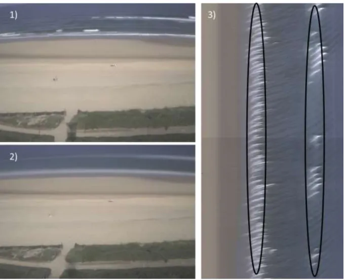
In spite of decades of research [e.g. Dolan and Davis, 1992; Sallenger, 2000; Coco et al., 2014; Karunarathna et al., 2014; Senechal et al., 2015], the immediate response of a beach system to storm event is still difficult to predict. This is because only wave contribution is generally considered to be the cause of shoreline changes. The modulation by sandbar and tide are often disregarded. Sandbars (Figure 1.2) are elongated shoals at wave-dominated coastlines commonly located parallel to the shoreline. The white bands offshore (Figure 1.2) indicate wave breaking on shallow bathymetry due to the presence of sandbars (outer and inner). The interface between the land and the water at mean sea level is digitised to mark the shoreline while the centers of the white bands are digitised alongshore (horizontally) and used as the sandbar location (Figure 1.2). Sandbars may result in less energy available to cause shoreline change (sheltering effect) and thus making the dynamics of the sandbar key to nearshore changes [van Enckevort and Ruessink, 2003, Vousdoukas et al., 2012]. Davis and Hayes [1984] indicated that beach morphology is not simply dependent on the absolute wave or tide, but also on the interaction between the two. While the importance of waves has been well documented, the influence of tides though recognised [Wright et al., 1984; Wright et al, 1987; Masselink and Short, 1993], is subtler and less understood. As a consequence, understanding and predicting shoreline change at barred beaches in mixed wave and tide environments remains a challenge due to the complex interactions between waves, tide [Davis, 1985; Masselink and Short, 1993] and sandbars [Banno and Kuriyama, 2012] as well as to previous conditions [Yates et al., 2009; Davidson et al., 2013], which usually are not directly accounted for.
18 Figure 1.2. A 10-min time exposure video image on September 4, 2008 from the camEra video system, Biscarrosse.
Different approaches have been used to investigate shoreline evolution. They include ground truth surveys of cross-shore profiles [Miller and Dean, 2007] using GPS [e.g., Morton et al., 1993; Ruggiero et al., 1999; Yates et al., 2009] or using airborne LIDAR systems [Sallenger et al., 1999; Stockdon et al., 2002]. These approaches cannot be performed dayly on the long term. Such surveys are typically performed monthly, which does not allow capturing short-term storm-driven changes. The most significant changes that typically occur during and immediately after storms can therefore be missed. In addition, conventional methods are restricted by storm surge and wave-induced setup and runup and usually cannot extend much beyond the low-tide waterline. In recent decades, shore-based video cameras have become increasingly popular for monitoring beach changes. This is because it can be used to build a database of frequent (~hourly), long-term (~years) and spatially-extensive observations of beach behaviour [Holland et al., 1997, Holman and Stanley, 2007; Holman and Haller, 2013]. Video systems perform satisfactorily under diverse conditions such as storms and fair weather, and capture information along the entire beach (~kilometers) including the geometry of the submerged morphology such as sandbars [Lippmann and Holman, 1989]. This disruptive method has promoted a better understanding of the hydro- and morphodynamics [Holman and Stanley, 2007; Holman and Haller, 2013]. It has also provided operational and real time observations [Coco et al., 2005; Pearre and Puleo, 2009] as well as
19 data to feed and validate numerical [Smith et al., 2007; van Dongeren et al., 2007; Davidson et al., 2013] and conceptual models [e.g. Turki et al., 2013]
This thesis is part of ARTS (‘Allocations de Rercherche pour une Thèse au Sud’) programmes, designed to strengthen research capacities in developing countries. Its purpose is to prepare young researchers to integrate the higher education and research systems of a developing country once they have finished their PhDs. In this work, the shoreline response at different scales to current and previous wave conditions is seen as an important concern for coastal users. This is compounded by the lack of adequate knowledge in the shoreline recovery, and the modulation of the shoreline variation by tides and sand bars. This work will contribute to increase our understanding of shoreline variability and its primary driver including frequency of storms and seasonal evolution, modulation of the storm impact and recovery by tide and sandbar, will help coastal managers appreciate shoreline evolution and better incorporate the impact of storms into Shoreline Management Plans (SMPs).
The main aim of this study is to develop a methodology to statistically assess shoreline resilience to storm events at different time scales for Atlantic conditions applied to storm-dominated mid-latitude (Biscarrosse, France) and storm-free tropical (Accra, Ghana) beaches.
In order to achieve this, 3 objectives have been defined.
i) Quantify shoreline resilience to storms and sequences of storms, under the modulation of tide and sandbar at Biscarrosse, SW France.
ii) Assess the two-dimensional (2D) and three-dimensional (3D) shoreline behaviour at multiple scales at Biscarrosse, SW France.
iii) Test a pioneering study on the influence of waves and tide on shoreline change at the microtidal Jamestown beach, Accra- Ghana.
1.3 Organization of Dissertation
The document is divided into 6 chapters and two annexes:
Chapter 2: Processes of coastal hydro- and morphodynamics. Previous studies on multi-scale coastal wave climate and morphodynamics are reviewed. Other forcings such as tide and sandbars are described.
20 Chapter 3: Study area, data and methods. Study areas, the intermediate meso-macrotidal Biscarrosse and microtidal James town beaches, are presented, though Biscarrosse is the principal site of this dissertation.
Chapter 4: Statistical approach of coastal response to storms. The impact of storms is investigated, together with the modulation of tides and cross-shore sandbar locations on storm impact and recovery rates, using a multi-linear regression analysis.
Chapter 5: Two and three-dimension shoreline changes at short and seasonal scales. Cross-shore migration and alongCross-shore deformation of Cross-shoreline are quantified through an empirical orthogonal analysis and combined with equilibrium shoreline modelling.
Chapter 6: Jamestown beach evolution under video surveillance. The potential for the extraction of waves, water level, and shoreline evolution is explored at the pilot site of Jamestown in Ghana over a 6-month period. Estimates are compared with hindcast data and main drivers of shoreline changes are identified
Chapter 7: Concluding remarks, discussion and perspectives Bibliography: Presents a list of the references cited in this work.
Annex: Contains a list of the different scientific contributions that resulted in the completion of this thesis and other extra researches.
21
2 Hydro-morphodynamic coastal processes
...It is astonishing and incredible to us, but not to Nature;
for she performs with utmost ease and simplicity
things which are even infinitely puzzling to our minds...
22 2.1 Wave dynamics in the nearshore: refraction, diffraction and breaking
2.2 Beach system
2.2.1 Bar-berm beach dynamics
2.2.2 Wave-induced short term morphodynamics 2.2.3 Tides and their control on nearshore processes 2.3. Shoreline dynamics
2.3.1 Shoreline definition: a review 2.3.3 Sandbar to shoreline coupling
2.4. Transient and persistent effect of storms
2.4.1 Wave climate and storminess: regional to beach scale 2.4.1.1 Wave climate
2.4.1.2 Storms 2.4.2 Storms impact 2.4.3 Post-storm Recovery
2.5 Shoreline acquisition and prediction
2.5.1 Different conventional shoreline measurement techniques 2.5.2 Video monitoring: context and background
2.5.2.a Video monitoring of the nearshore: 25 years of developments and use 2.5.2.b Shoreline and sandbar from video
23 2.1 Wave dynamics in the nearshore: refraction, diffraction and breaking
Waves in deep water are sinusoidal in form. Ideal wind waves in sinusoidal motion are typically characterized by a point of maximum elevation, i.e. the wave crest, and a point of minimum elevation, the trough [Davidson-Arnott, 2010]. The dynamics of waves from deep water to the nearshore (defined here as the region where waves are significantly affected by the bottom) is crucial to estimate inshore wave characteristics. In the nearshore, waves undergo changes due to shoaling, diffraction, refraction and depth-induced breaking and can move sediment and affect the seabed morphology, particularly during storms [Weaver and Slinn, 2010].
Waves bend towards shallow water along the beach due to refraction; a process in which the wave crests tend to parallel (Figure 2.1a) the depth contours and waves breaking parallel to the shoreline. Obliquely-incident breaking waves generate longshore currents that cause alongshore sediment transport. Diffraction (Figure 2.1b) occurs for large along-crest wave energy gradients. Wave diffraction is important in ports, harbours or around offshore islands.
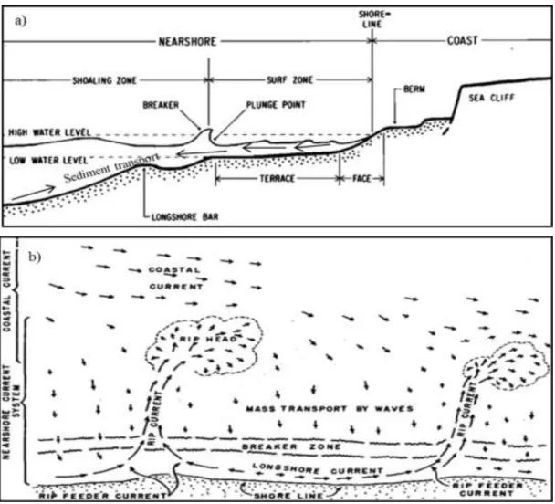
The nearshore can be categorised into 3 distinct zones [Short, 1986] namely wave shoaling seaward of the breaker point, a surf zone of breaking waves and a swash zone of final wave dissipation on the upper beach (Figure 2.2a). The nature and extent of each of these zones ultimately determine the beach changes. The width of the shoaling, surf and swash zones, are functions of sediment size and wave height [Dean and Dalrymple, 2002]. Nearshore wave breaking, which is a widely known activity [Dean and Dalrymple, 2002; Svendsen, 2006; Davidson-Arnott, 2010] is also responsible for energy dissipation and sediment movement. Generally, waves break as they reach a limiting steepness of wave height to depth ratio γ = hb/L, [Svendsen, 2006; Davidson-Arnott, 2010].
24 Figure 2.1 a) Wave refraction causes wave fronts to parallel the shape of the coastline as they approach shore and encounter ground (courtesy of google images) b) wave diffraction around a exposed feature; waves bend after passing an obstacle
These breaking waves exist in different forms namely spilling, plunging, surging and collapsing breakers [Iribaren, 1949; Battjes, 1974; Wang et al., 2002] which have been estimated based on the non-dimensional surf zone similarity parameter ξb [Battjes, 1974].
ξb = tanβ (
𝐻𝑏
𝐿) −0.5
(2.1)
where β is beach slope, hb is depth at breaking, L is deep water wavelength and Hb is the breaker height.
Though the breaker type is difficult to generalise on a non-uniform bathymetry, on alongshore-uniform beaches, breaker type is classified as surging/collapsing (ξb > 3.3), plunging (0.5 < ξb < 3.3) and spilling
(ξb< 0.5) [Iribaren, 1949; Galvin, 1968; Battjes, 1974]. Plunging waves are characterized by an arched
shape with a convex back and a concave front (seen on Figure 2.2a).
After breaking, the wave energy is dissipated over a variable cross-shore distance, a process that causes turbulence in the breaker zone. Besides, a surf bore is created as the top of the wave forms an air bubble between the crest and the plunging top. The kind of breaking, however, depends on the bottom topography. On barred beaches it is seen that after the first breaking the energy dissipation becomes zero as the water depth behind the bar increases and it is kept as zero until the next breaking occurs [Wanatabe, 1988]. An important factor in the breaking process is also in the wave height and the water level that
25 determine the position of breaking. Shoaling occurs when the progressive wave encouter the seabed. If the water level is too high and the waves are not encoutering the seabed, shoaling will not occur and the waves do not break. At steep beaches, plunging or surging wave breaking occurs on the upper beach, while gently sloping beaches produce a spilling breaking over wide distances to dissipate wave energy [Galvin, 1968; Svendsen, 2006; Davidson-Arnott, 2010].
Figure 2. 2 a) schematic typical beach profile, terminology and zonation b) Schematic diagram of surface flow in coastal and nearshore current systems. Length of arrows indicates their relative magnitudes [Source: Shepard and Inman, 1951].
When water run up on anyone standing on a beach, they often feel the water tugging the sand away from under their feet, due to a force called undertow. This undertow is a wave-induced current, generated to compensate for the shoreward mass flux of the waves. Near the bed, it interacts with wave motion to dictate the amount of sediment put in suspension, after wave breaking. In the water column, it moves sediment offshore, counteracting the suspended flux due to waves. Hence, this current is crucial in
26 determining the amount and direction of sediment movement in nearshore regions [Guannel and Ozkan-Haller, 2014].The breaking of waves in the nearshore results in changes of the wave-induced momentum that drive nearshore currents and pressure gradients [Maa et al., 2001]. Hence understanding these flows is a prerequisite to predicting morphological change. Besides, the mean breaking-wave driven nearshore circulation has a complex three-dimensional structure even on relatively simple bathymetry.
Breaking waves may generate strong offshore flows often call rip currents (Figure 2.2b) when waves push water up the beach face. If there is an area where the water can flow back out into the ocean more easily, such as a break in the sand bar, then a rip current can form. These are strong, offshore-directed currents known to pull the water (or sediments) at all water depths through the surf zone and dissipates offshore of the breaking waves. These are also essential currents for nearshore management.
In general, observed breaking induced currents contain substantial fluctuations [Raubenhimer, 2004] at infragravity periods (about 1 minute) that appear to result from a combination of gravity and vorticity (e.g. shear) waves, but the generation mechanisms and overall significance of these low frequency motions are largely unconsidered. One possible reason for this is lack of nearshore wave conditions. For example, on most study sites breaking waves are used [e.g. Maa et al., 2001; Guza and Feddersen, 2012; Splinter et al., 2014a] though breaking waves are usually obtained from mathematical relations [e.g. Larson et al., 2010] through some sporadic means.
2.2 Beach system
2.2.1 Bar-berm beach dynamics
One approach to the quantification of beach morphology has been the identification of sets of morphologic states. Investigations have long showed that beaches experience distinct seasonal onshore/offshore transport of sand
[
Shepard, 1950; Shepard and Inman, 1951]. A simple but well-known example of such parameterisation is the summer-winter (or bar-berm) model[
e.g. Shepard, 1950], based on observations that the shape of many beaches tends to change from unbarred to barred profiles (Figure 2.3). The beach is considered only in a one-dimensional structure of erosion or accretion; the basic beach profiles attainable are the swell profile formed when the waves are of low steepness and the barred profile or storm profile formed when the waves are of high steepness. Variation of forcing conditions results in uniform sediment movement onshore/offshore. It is assumed that the exchange of material between the bar and the berm takes place under conservation, that is, no material is lost offshore. The volume eroded from the berm is assumed stored in one offshore bar (or, representative morphological volume) that will reach a certain equilibrium bar volume if the wave conditions are steady and the grain size does not vary.27 If the bar volume at any given time is smaller than the equilibrium volume, then the sandbar volume will grow, and vice versa. From Figure 2.3, we see that growth in bar volume causes the corresponding decrease in berm volume (and shoreline retreat), and decay in bar volume causes increase in berm volume (and shoreline advance). Alongshore-averaged (or two-dimensional 2D) cross-shore sandbar dynamics can thus be considered as morphologic adjustment to the hydrodynamic forcing
[
Aagaard et al., 1998], and more precisely the convergence of sediment transport at the breakpoint.Figure 2.3. Seasonal transformation from a summer beach (lower plot) to a winter beach (upper plot), accessed on 26/01/2016 on Google search.
Longshore bars are common features at wave-exposed beaches, and have influence on the foreshores
[
Takeda and Sunamura, 1992]. They also constitute the dominant mode of bed variability in the submerged nearshore area. While annual cycles are observed at most coastlines, with offshore migration during energetic winter months, significant changes also occur on a much shorter time scale, especially in response to storms. It has long been known that during storms or energetic conditions, sandbar moves seaward (through undertow current) and moves landward during low energetic conditions[
Birkemeier, 1984; Gallagher et al., 1998; Hoefel and Elgar, 2003] as shown in Figure 2.4. Additionally, seasonal trends in sandbar location can often be observed, whereby a sandbar is located more seaward28 after autumn and winter months with high waves than after the low-wave spring and summer months. It has also long been established that sandbar strongly controls the wave breaking location
[
Lippmann and Holman, 1989; Plant and Holman, 1998; Ruessink et al., 2007] and, hence, cross-shore sediment transport patterns; this may reinforce or suppress further bathymetric modifications[
Plant et al., 2001] through a feedback on hydro-morphodynamics. For instance, wave-breaking across an outer bar affects the hydrodynamics and hence the evolution of an inner bar. Sediment transport will be affected by the incidence of obliquely breaking waves (they lead to longshore transport) and the kind of sandbars that occur.Figure 2.4. Sandbar migration during storms and non-storm period. Upper panel: rapid offshore movement of sandbar resulting from ten stormy days [Gallagher et al., 1998]. Lower: slow onshore migration of the outer bar during a six month period of low wave conditions [Birkemeier, 1984].
Lippmann and Holman [1990] identified that the most frequently observed sandbar morphologies are the longshore-periodic (rhythmic) bars where linear bars occur under highest wave conditions, though unstable (mean residence time = 2 days). The study found out that shore-attached rhythmic bars were the most stable (mean residence time of 11 days) and generally form 5-16 days following peak wave events. Non-rhythmic, three-dimensional bars are very transient (mean residence time = 3 days), making the
29 beach changes more complex than the usual 2D-structure. Given that transitions to higher states occur under rising wave energy among the possible higher beach states, this suggests that up-state, erosional transitions (based on offshore bar migration) are better described by an equilibrium model where response is better correlated with incident wave energy than with preceding morphological state. Therefore, further understanding is required especially in regions where tide range and wave conditions are very comparable.
2.2.2 Wave-induced short term morphodynamics
Numerous attempts [Wright and Short, 1984;Hansen and Barnard, 2010; Splinter et al., 2014b] have been made to relate short term (daily or weekly) fluctuations in the wave field with beach changes. Notably, Wright and Short [1984] developed an empirical predictive model to relate beach states to the dimensionless Dean parameter, Ω. In order to understand the complexity of the beach due to variation in forcing and morphology, they used Ω [Goulay, 1968] given in Eq. 2.2 to classify three distinctive beach types based on the wave breaking height Hb, period T, and sediment characteristics (the sediment fall
velocity ws):
𝛺 = 𝐻𝑏
𝑊𝑠𝑇 (2.2)
Wright and Short [1984] showed that the three distinctive beach states are related to Ω with Ω>6, 1< Ω<6 and Ω < 1 for dissipative, intermediate and reflective beaches, respectively. In this classification, these three beach states are subdivided into six commonly occurring beach states: dissipative, longshore bar trough (LBT), rhythmic bar and beach (RBB), transverse bar and rip (TBR), low-tide terrace (LTT), and reflective. Following this beach classification by Wright and Short [1984], a beach cannot be resumed to a pure cross-shore profile evolution but present irregularities in the longshore due to variation in forcing (Figure 2.5).
As indicated earlier, the cross-shore beach dynamics can be of an alongshore uniform (or two-dimensional, 2D) character and reflect overall on/offshore shoreline migration depending on the energy incident on the beach. Variation of the beach cross-shore position, for example the isolevel position, is a clear and easily-understood indicator of beach accretion and erosion, with seaward and landward migration, respectively. From Wright and Short [1984], beaches are mostly 2D for very energetic conditions or 3D for intermediate conditions. In the 2D state, the beach varies minimally or not all alongshore (Figure 2.5a). By the Wright and Short model, a beach can therefore have 2D patterns if it is in the dissipative or reflective state. In times when larger amount of energy due to forcing occurs, erosional sequences [Short, 1999] could cause the beach state to jump to the dissipative state within hours
30 [Lippmann and Holman, 1990; Van Enckevort and Ruessink, 2003; Ranasinghe et al., 2004]. In the dissipative state (Figure 2.5a), it is believed that there would be the removal of berm feature yielding a 2D profile and the development of bar type profiles. Simply, beach cusps are non-existent or minimal while the beach now shows no alongshore variations. In the dissipative state, the beach is gentle and is characterized by wide surf zone. On the other hand, during the reflective state (Figure 2.5f) when wave conditions are weak, the beach becomes steep with berms prograding seaward to give a wider beach and narrow surf zone leaving the beach in 2D form. The trends and prediction of 2D positions are therefore tricky because the beach state can only be identified by its modal state [Wright and Short, 1984]; in other words the present beach state is determined by the recent history of both the wave field and the beach morphology.
During an accretionary (downstate) sequence with decreasing energy, the 2D dynamics turn into 3D as the beach advances through several intermediate states, from high energy dissipative members towards the reflective state over a number of days to weeks [Lippmann and Holman, 1990; Van Enckevort et al., 2004] and become 2D again. In the intermediate state of moderate to high energy, the longshore beach component is alongshore non-uniform (or three-dimensional, 3D) and mostly corresponds to changes in the non-uniformities in the shoreline. 3D shoreline development are associated with periodic developments such as cusps [Coco and Murray, 2007] or forced pattern from sandbar irregularities (Figure 2.5b to e) that form during the intermediate states according to the Wright and Short classification. With characteristic rip circulation, dynamic bar forms, abundant surf zone and beach sediment and moderate waves, they can undergo rapid changes as wave height fluctuates causing rapid reversals in onshore-offshore and alongshore sediment transport [Wright and Short, 1984].
Increasing in energy and irregularity, the intermediate states are identified as LTT, TBR, RBB, and LBT (Figure 2.5b to Figure 2.5e). Wright and Short [1984] show that the intermediate beaches exhibit complex morphologies with increasing three dimensionality due to structures such as the bar-trough topography or bathymetry, formed during the mechanism of an up or downstate. As explained earlier, sandbar dynamics may therefore be significant for the nearshore complexity as sandbar moves about beneath the water, altering the movement of waves and water depth. Recently, Stokes et al. [2015] additionally showed that a tidally-modulated wave power term may influence the rate of morphological change, like the 3D dynamics. Besides, given this likely interaction between 2D sandbar and shoreline, it is possible to hypothesise that sandbar positions can affect 3D shoreline variations and the larger nearshore dynamics.
31 Figure 2.5. Plan and profile configurations of the six major beach states [Wright and Short, 1984; Short, 2006] based on the dimensioless Dean parameter Ω = Hb/wsT. From (a) to (f), we have decreasing energy
and Ω, respectively for dissipative, LBT, RBB, TBR, LTT and reflective states.
2.2.3 Tides and their control on nearshore processes
Astronomical tides drive substantial modulation of wave action on beach dynamics and subsequent beach types (Figure 2.6). Beaches are classified as microtidal (<2 m), or meso-tidal (2-4 m) or macro-tidal (> 6 m) based on the tide properties [Davies, 1964; Masselink and Short, 1993; Short, 1996].
32 Micro-tidal beach systems are assumed to be wave dominated, with a low tide range that has a minor to negligible role in determining beach morphology. Tide is therefore largely ignored in assessing general beach morphodynamics. At microtidal beaches, the swash, surf and shoaling zones are therefore assumed to be stationary [Short, 1996]. In contrast, tide range is important on macro-tidal beaches as it could result in the formation of multiple sandbars and changes in swash processes. When waves suspend sediment in the narrow surf zone, inducing pulse-like high sediment concentration in shallow water, the suspended sediment can be advected by the tidal current causing erosion [Shi et al., 2013). Davidson and Turner [2009] found that increasing the tidal range diminishes the bar amplitude and spread it out across the profile. The impact on shoreline erosion is thus lessened by increasing the tidal range TR, as the impact is distributed over a broader region of the profile.
Generally, small tidal range is expected to increase surf zone and swash processes and thus to result in rather short response times to time-varying incident wave conditions, whereas a large meso- to macro-tidal range favours shoaling-wave processes and, hence, increases the response time. The significance of tidal oscillations for the beach morphodynamics can be quantified by the ratio of tidal range to wave height [Masselink and Short, 1993; Short, 1996; Masselink et al., 2006]. For values of the relative tide range (RTR, Eq. 2.3) exceeding 5-10, morphodynamic effects of tidal translation is significant [Masselink and Short, 1993].
𝑅𝑇𝑅 = 𝑇𝑅𝐻
𝑏 (2.3)
From equation 2.2 and equation 2.3, the RTR can be linked to the dimensionless fall velocity, Ω that Wright and Short [1984] took to describe the beach states:
Ω = 𝑇𝑅
𝑅𝑇𝑅(𝑊𝑆 𝑇) (2.4)
This formulation suggests that increasing RTR values result in low Ω and reflective beaches, while decreasing values may result in more dissipative beaches. Landward of the breaker zone, single bar beaches are dominated by surf and swash zone processes. This is not always so especially on two or multiple barred beaches [Masselink and Short, 1993; Short, 1996]. As tide range increases the impact of both the swash and surf zone processes decreases. The RTR values do define tide-dominance when the values are large and wave-dominance when RTR values are small. For each tidal cycle, the maximum Hb
can be considered representative of the breaker condition; even during energetic waves and large tides. Masselink and Short [1993] as well as Short [1996] reviewed that when Ω>1 or RTR < 5 the formation of sandbars is prevalent, whereas when Ω<1, there is formation of berm under dominant onshore transport (Figure 2.6).
33 Figure 2.6. Conceptual beach model [Masselink and Short, 1993]. The Beach state is a function of the relative tide range (RTR = TR/Hb). HT and LT refer to mean high tide and mean low tide levels,
respectively.
In addition, the formation of an intertidal bar around the mid-tide position during low-wave conditions and neap tides can be triggered by a reduction in TR but not the rise in Hb. For example, a new forcing
parameter, Hydrodynamic Forcing Index (HFI), has been proposed that allows representing the cumulative effect of wave and tide forcing [Almar et al., 2010]. The HFI index is defined as the ratio of offshore significant wave height Hs to the (averaged over a tidal cycle) lowest offshore water level dmin
experienced over a tidal cycle above the lowest astronomical tide (LAT):
HFI =𝑑𝐻𝑠
𝑚𝑖𝑛 (2.5)
This HFI parameter is somewhat more suited to storm impact than the RTR at the time scale of storms as HFI is high during a storm, which is not necessarily the case for RTR.
34 2.3 Shoreline dynamics
2.3.1 Shoreline definition: a review
The shoreline has been broadly investigated and defined [e.g. Crowell et al., 1991; Moore et al., 2000; Stockdon et al., 2002]. Shoreline is commonly identified with indicators (proxies) based on geographical, morphological or hydrodynamical considerations [e.g. List and Farris, 1999; Zhang et al., 2002; Stockdon et al., 2002]. The shoreline can be defined at the location of the waterline identified by a change in colour or gray tone caused by differences in water content around it or a line of seaweed and debris. For some, shoreline is the seaward edge of the vegetation. Boak and Turner [2005] reviewed these proxies (Figure 2.7) into visually discernible coastal features (e.g. high water lines, HWL) and specific tidal datum (the intersection of the coastal profile with a specific vertical elevation, e.g. mean high water, MHW line).
The HWL, which delineates the landward extent high tide watermark, is commonly chosen as the shoreline. However, a vast number of studies [Crowell et al., 1991; Moore et al., 2000; Stockdon et al., 2002] indicate difficulties in interpreting HWL from aerial photographs. In addition, on a low-sloping beach the horizontal offset of the shoreline indicator HWL due to wave, tide, or wind effects can be on the order of several tens of meters [Thieler and Danforth, 1994].
On the other hand, tide-coordinated or datum-based shorelines based on tidal elevation generally consist of the position of a specified elevation contour. Figure 2.7 (lower section) shows an example of the shoreline definitions based on tidal datums [Plant and Holman, 1997; Madsen and Plant, 2001; Aarninkhof et al., 2003; Kingston, 2003; Moore et al., 2006] commonly used with digital detection techniques (e.g. video images). The shoreline is defined at the interface between the beach and the sea only at the selected tide (elevation contour). Despite this, unlike microtidal beaches, on meso- to macrotidal barred beaches it is not straightforward to select the elevation that best represents the overall beach response. In line with this, Castelle et al. [2014] recently found out that the intersection of the coastal profile with the MHW level is an effective shoreline proxy for meso- to macrotidal, high-energy, multiple-barred beaches. Due to its location on the upper beach, the inner-bar and berm dynamics have little influence on the shoreline estimation. Such selection is also motivated by previous findings at Ocean Beach where changes in the MHW and MSL shoreline proxies are well correlated (R = 0.9 for most of the beaches) to volumetric change [Hansen and Barnard, 2009; List and Farris, 2007].
35 Figure 2.7. Shoreline indicators based on specific tidal datums (upper plot). On the lower plot are tidal datums used along the New South Wales coastline, Australia [adapted from Boak and Turner, 2005] as proxy for shoreline.
2.3.2 Sandbar and shoreline coupling
Sandbars reduce the amount of wave energy reaching the shoreline by limiting the wave height through breaking. The coupling between sandbar and the shoreline may be linked to the distance between the sandbar and the shoreline [e.g. Sonu, 1973; Wright and Short, 1984; Van de Lageweg et al., 2013]. Sonu [1973] observed an out-of-phase relationship of inner bar and shoreline patterns, i.e. an inner bar bay facing a seaward bulge in the shoreline. An in-phase relationship can also sometimes be observed with an inner bar horn facing a seaward bulge in the shoreline [Castelle et al., 2010; Price and Ruessink, 2011]. The relationship between inner- and outer bar patterns is reminiscent of the more commonly observed relationship between inner bar patterns and shoreline rhythms [e.g. Wright and Short, 1984; Coco et al., 2005; Thornton et al., 2007]. In a related study, Davidson and Turner [2009] identified that
36 when the bar is lower in amplitude and located closer to the shoreline, it lessens shoreline erosion. Several processes and physical parameters have been hypothesised to affect the sandbar-shoreline coupling. Birkemeier [1984] showed that the beach profile configuration is modified by the location and horizontal movements of the sandbar crest. That large change to the profile in terms of volume movements always resulted in significant sandbar movement.
One parameter that links this sandbar and the morphology is the beach steepness (slope) parameter, γ (defined as hb/L in section 2.1); it dictates where the wave breaks on the beach. Recent works
[e.g. Davidson and Turner, 2009] have shown that increasing γ can move the bar progressively shoreward, while decreasing γ causes a seaward translation. However, Davidson and Turner [2009] found that on average, varying γ has negligible impact on the shoreline evolution. From Davidson and Turner [2009] review, it is deduced that although the shoreline and sandbar sections of the profile could be coupled in the sense that erosion of sediment from the shoreface is deposited on the sandbar, it is still insufficient to substantiate that enhanced dissipation over a developed sandbar might reduce energy levels at the shoreline relative to erosion. Interestingly, no increase in sandbar width was seen to impact the shoreline evolution. In essence, this indicates not all sandbar characteristics affect the shoreline. Another parameter, the sandbar crest depth variability, though important [Coco et al., 2005; Ruessink et al., 2007] maybe less useful as an indicator of sandbar activity on the shoreline, since large sandbar movements occur with little or no change in crest depth. However, Pruszak et al. [2011] revealed that the location of the inner sandbar and the shoreline can exhibit a reasonably high correlation showing their onshore/offshore movements are very consistent even if in the outer sandbar region the location of the outer bars subsystem is much less correlated with the shoreline position. Finally, the angle of wave incidence has been suggested to affect the phase of coupling of shoreline and sandbar since larger angle of incidence drive strong longshore currents, while longshore currents destroy sandbar variability [Price and Ruessink, 2013].
There seems to be some debate as to how and what is associated to sandbar to shoreline coupling. Although the variability of bars and their links to environmental factors has been the objective of many analyses, the direct interactions between sandbar and the shoreline still seem to be insufficiently identified. The relation between the sandbar and the shoreline could be more complex due to the presence multiple sandbars, as there can be interaction between the inner bar and outer bar [e.g. Castelle et al., 2010; Price and Ruessink, 2013]. At present, previous models and methods have not explained the quantitative content of the sandbar in relation to shoreline change in comparison to other parameters such as the waves and tides and antecedent conditions. The link between shoreline and sandbar location is sketchy as we found in the literature. For instance the relative contribution of the sandbar location to
37 shoreline changes during storms in isolation and during recovery has not been clearly observed in the literature. Questions like how the sandbar to shoreline distance will influence beach recovery magnitudes and recovery duration can be used to establish a relation between the location of sandbar and the shoreline.
2.4. Transient and persistent effect of storms
2.4.1
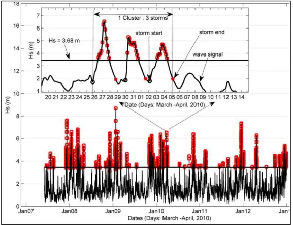
Wave climate and storminess: regional to beach scale 2.4.1.a Wave climateWaves are the main driver of nearshore hydro-morphodynamics and are generated by wind either locally or from distant location. The height and period of the waves depend on the speed and duration of the generating winds and the fetch. The types of waves that break on a beach and their seasonal variance are known as the wave climate. Several findings suggest that along wave-dominated coastlines, the impact of regionally-varying wave climates will have a more significant impact in the coming decades and cannot be ignored in forecasting future shoreline variability [Brunel and Sabatier, 2009; Ranasinghe et al., 2012; Ruggiero, 2013]. In light of this, offshore and coastal wave climate evolution is particularly important for human activities at high energetic regions (e.g. Bay of Biscay and the French Atlantic coast). To achieve this, the storminess (intensity and recurrence of storms) [Masselink and van Heteren, 2014] and wave seasonality are key.
In the last half-century, the variation in wave climate has been analysed along the North Atlantic. Wang and Swail [2001] detected an upward trend in seasonal extremes of Hs from 1958-1997, where higher rates occur in winter. Dodet et al. [2010] investigated the variability in the North-East Atlantic Ocean (25°W-0°W and 30°N–60°N), with hindcast (1953–2009) waves. They detected strong seasonal and inter-annual fluctuations of wave climate, with winters characterized by large and long-period waves of mean direction spreading from south-west to north-west, and summers characterized by smaller and shorter-period waves originating from northern directions. From northern (55°N) to southern (35°N) latitudes, the significant wave height (Hs) decreases by roughly 40%, the mean wave direction rotates clockwise by about 25% while the peak period (Tp) only grows by 5%. Linear trend analysis between these years showed spatially variable long-term trends, with a significant increase of Hs (up to 0.02 m/yr) and a counterclockwise shift of direction (up to -0.1° per year) at the northern latitude, contrasting with a fairly constant trend for Hs and a clockwise shift of direction (up to +0.15° yr) at southern latitudes, while in the long-term trends of Tp are less significant. This variation in the trend of wave parameters is very significant especially when wave effect dominates the beach processes.
38 Using dynamical and statistical methods [Charles et al., 2012; Laugel et al., 2014], projected wave heights, periods and directions have been analysed at regional scale along the coast of the Bay of Biscay. Clockwise shift of winter swell directions is linked to the intensification and the northeastward shift of strong wind core in the North Atlantic Ocean. As offshore changes in the wave height and the wave period as well as the clockwise shift in the wave direction continue toward the coast, it would impact the coastal dynamics by reducing longshore wave energy. Similarly, the large scale spatial variability of sea states at the French Atlantic coast was assessed by Butel et al. [2002] using wave rider time series at Biscarosse (in 26 m depth). 3D histogram distributions (Figure 2.8) of significant wave heights, periods and directions indicate that a wide range of wave directions and age can be measured at Biscarosse, mainly due to atmospheric forcing.
Figure 2.8. Left: 1-D histograms of significant wave height (Hs) and, Right: mean period (Tp). Gray shade is for Biscarosse, dashed surface is for Yeu, and white with thick lines is for Biscay after Butel et al. [2002].
It is shown that Biscarosse beach, a characteristic of most of the beaches encountered in the SW France is exposed to long and energetic waves originating mainly from the W-NW. During fall and winter seasons (typically November to March) the mean significant wave height and mean period are high while during spring and summer (typically April to October) the mean significant wave height is low [Butel et al., 2002]. Woolf et al. [2002] established a relationship between wave height anomalies and large scale atmospheric pressure patterns over the Northeast Atlantic on the basis of satellite altimetry. More precisely they attributed part of the variability to the North Atlantic Oscillation (NAO) and secondarily to the East Atlantic Pattern (EA). In most cases, North Atlantic Oscillation (NAO) and other climatic indices
![Figure 1.1. Beach system, showing the use of coastal environments [credit: google images]](https://thumb-eu.123doks.com/thumbv2/123doknet/14731315.573032/18.918.209.752.212.574/figure-beach-showing-coastal-environments-credit-google-images.webp)


![Figure 2.10. Different time exposure images from around the world (a) Biscarrosse (b) Gold Coast [Plant et al., 2007] (c) Jamestown, Ghana (d) Duck [Plant et al., 1999]](https://thumb-eu.123doks.com/thumbv2/123doknet/14731315.573032/48.918.122.803.482.991/figure-different-exposure-images-biscarrosse-coast-plant-jamestown.webp)