HAL Id: insu-01682118
https://hal-insu.archives-ouvertes.fr/insu-01682118
Submitted on 27 Apr 2018
HAL is a multi-disciplinary open access
archive for the deposit and dissemination of sci-entific research documents, whether they are pub-lished or not. The documents may come from teaching and research institutions in France or abroad, or from public or private research centers.
L’archive ouverte pluridisciplinaire HAL, est destinée au dépôt et à la diffusion de documents scientifiques de niveau recherche, publiés ou non, émanant des établissements d’enseignement et de recherche français ou étrangers, des laboratoires publics ou privés.
Sources, Load, Vertical Distribution, and Fate of
Wintertime Aerosols North of Svalbard From Combined
V4 CALIOP Data, Ground-Based IAOOS Lidar
Observations and Trajectory Analysis
Claudia Di Biagio, Jacques Pelon, Gérard Ancellet, Ariane Bazureau, Vincent
Mariage
To cite this version:
Claudia Di Biagio, Jacques Pelon, Gérard Ancellet, Ariane Bazureau, Vincent Mariage. Sources, Load, Vertical Distribution, and Fate of Wintertime Aerosols North of Svalbard From Combined V4 CALIOP Data, Ground-Based IAOOS Lidar Observations and Trajectory Analysis. Journal of Geophysical Research: Atmospheres, American Geophysical Union, 2018, 123 (2), pp. 1363-1383 �10.1002/2017JD027530�. �insu-01682118�
Sources, load, vertical distribution, and fate of wintertime aerosols north of
Svalbard from combined V4 CALIOP data, ground-based IAOOS lidar
observations and trajectory analysis
C. Di Biagio*, J. Pelon, G. Ancellet, A. Bazureau, V. Mariage
LATMOS/IPSL, UPMC Univ. Paris 06 Sorbonne Universités, UVSQ, CNRS, Paris, France
*
Now at Laboratoire Interuniversitaire des Systèmes Atmosphériques (LISA), UMR CNRS 7583, Université Paris Est Créteil et Université Paris Diderot, Institut Pierre et Simon Laplace, Créteil,
France
Corresponding author: Claudia Di Biagio (claudia.dibiagio@lisa.u-pec.fr)
Key points
Combining CALIOP satellite and IAOOS local‒scale lidar observations allows to better characterize properties and transport of Arctic aerosol
Dust‒type aerosols are overrepresented in CALIOP Arctic dataset, and a large part of it is most probably corresponding to diamond dust
The V4 CALIOP 532 nm aerosol extinction is a factor 2 lower than averages reported by Di Pierro et al. (2013) using V3 dataset
Abstract
We have analyzed aerosol properties at the regional scale over high Arctic north of Svalbard between October 2014 and June 2015 from version 4 (V4) CALIOP (Cloud and Aerosol Lidar with Orthogonal Polarization) space-borne observations and compared results with surface lidar observations from IAOOS (Ice-Atmosphere-Ocean Observing System) platforms. CALIOP data indicate a maximum in aerosol occurrence at the end of winter attributed to low‒level (0-2 km) and mid‒tropospheric (2-5 km) particles identified in CALIOP V4 product as being mostly of dust origin. Another maximum was observed in October‒December attributed to clean marine particles below 2 km and smoke and dust above. The 532 nm aerosol extinction was in the range 1-8 Mm-1 (0‒2 km), 1-18 Mm-1 (2‒5 km), and 0-6 Mm-1 (5‒10 km), a factor 2 lower compared to values previously reported using CALIOP V3 dataset. Aerosols are identified from trajectory analyses to originate mostly from Russia/Europe at all altitudes, and also North America above 2 km, and it is concluded that dust and clean marine types are most probably overrepresented in the analyzed CALIOP dataset. It is proposed that most part of dust types are diamond dust, while part of clean marine are polluted species, as corroborated from co‒located polarized lidar IAOOS observations. IAOOS observations allowed confirming the identified sensitivity of CALIOP with a particle backscatter coefficient of ~0.001 km-1sr-1 at 532 nm. For optically thicker layers CALIOP is shown to be a valuable tool to follow transport of aerosol layers in the Arctic and identify their possible modifications.
Index terms: 0305, 0345, 0368, 3311, 3360
1. Introduction
The Arctic is the region of the Earth undergoing the fastest climate changes, and one of the key issues is to better monitor ongoing modifications and understand their consequences. Changes in Arctic climate are linked to local, regional, and large scale processes [Döscher et al., 2014] and have an influence on the global surface energy and moisture budgets, atmospheric and oceanic circulations, and geosphere‒biosphere interactions [McGuire et al., 2006]. Dynamical latitudinal interactions concur to the Arctic warming amplification [Pithan and Mauritsen, 2014] and induce strong meteorological variability. By consequence, this is the region where global and regional models and reanalyses show their largest uncertainties [Tjernström et al., 2008; Lidsay et al., 2014]. Henceforth, it is recognized that an important source of this uncertainty comes from atmospheric aerosols [Law and Stohl, 2007; Quinn et al., 2009; Law et al., 2014; Gagné et al., 2015]. Aerosols in the Arctic are both from long‒range transport and local emissions and include both natural and anthropogenic species [Rahn et al., 1977; Warneke et al., 2009; Matsui et al., 2011; Ancellet et al., 2014; Becagli et al., 2016; Aliabadi et al., 2016]. Despite their considerable lower load compared to mid‒latitudes (the daily optical depth rarely exceeds 0.2, Tomasi et al. [2012]), aerosols have been demonstrated to importantly affect the radiative budget of the Arctic through complex interactions with clouds and radiation [e.g., Ritter et al., 2005; Garrett and Zhao, 2006; Stone et al., 2007; Bourassa et al., 2013]. The quantification of long range transport of pollution to the Arctic and its radiative impact has in particular been re-emphasized by recent analyses [Acosta Navarro et al., 2016] and remains a key issue, especially during wintertime when observations are rather limited.
The sources of long-range transported aerosols and local particles, their spatial and seasonal distribution, their physico-chemical and optical properties, and direct and indirect effects have been the object of a large number of studies in the recent years [Iziomon et al., 2006; Tomasi et al., 2007; Quinn et al., 2009; Jacob et al., 2010; deVilliers et al., 2010; Stone et al., 2010; Brock et al., 2011; Di Biagio et al., 2012; Tunved et al., 2013; Law et al., 2014; Croft et al., 2016; Young et al., 2016; Zamora et al., 2016; Huang et al., 2017; among others. See also the recent AMAP (Arctic Monitoring and Assessment) report, AMAP [2015], for an executive summary of Arctic short‒lived climate forcers and their impacts]. These studies mostly refer to data acquired from ground‒based coastal stations allowing for systematic observations, as in Ny-Ǻlesund in Svalbard [Tunved et al., 2013], or intensive ship-based or airborne field campaigns both close to the coasts and across the Arctic Ocean (i.e., the FIRE Arctic Cloud Experiment (FIRE-ACE) and the Surface Heat Budget of the Arctic Ocean (SHEBA) in 1998-1999; during the IPY three major field experiments took place in 2007-2008: the Arctic Research of the Composition of the Troposphere from Aircraft and Satellites (ARCTAS), the Arctic Summer Cloud Ocean Study (ASCOS), and the Polar Study using Aircraft, Remote Sensing, Surface Measurements and Models, of Climate, Chemistry, Aerosols, and Transport (POLARCAT); more recently, in spring 2013, the Aerosol Cloud-Coupling and Climate Interactions (ACCACIA) took place). Despite the invaluable significance of these data, they have two strong weaknesses: part of them are representative mostly of a “past” Arctic (i.e., FIRE-ACE and SHEBA were performed about twenty years ago) and so not adequate to represent new Arctic conditions (new aerosol sources and
pathways, thinner and younger Arctic sea ice, etc.); whereas others have a limited temporal coverage (weeks to months), which prevents from fully investigating seasonal processes. Field data on wintertime aerosols are mainly related to the measurements performed in the stations of the International Arctic System for Observing the Atmosphere (IASOA) over land (https://www.esrl.noaa.gov/psd/iasoa/observatories), that can be used as near surface reference observations. They mainly show that aerosol mass is maximum in spring (March-April) at Mount Zeppelin (474 m a.s.l.) in Svalbard [Tunved et al., 2013]. Pollution aerosols occurring during this period have been identified to be linked to the formation of arctic haze [Quinn et al., 2009]. Aerosol-cloud interactions can also lead to diamond dust (tiny ice crystals) formation. They are rather frequently observed in the Arctic mostly near the surface (more than 10% of the time between November and May during SHEBA) where they led to a low radiative impact [Intrieri and Shupe, 2004]. This is however still an area of investigation and characteristics as well as interaction processes need to be better characterized to ascertain their impact [Girard and Blanchet, 2001].
New space lidar observations provide a more continuous coverage of the Arctic and the Arctic Ocean with the measurement of some key variables all year‒round including wintertime in the whole troposphere. The Cloud-Aerosol Lidar and Infrared Pathfinder Satellite Observation (CALIPSO) mission [Winker et al., 2010] has proven to be very efficient at investigating the distribution, load, and transport of aerosols in the Arctic [de Villiers et al., 2010; Di Pierro et al., 2011, 2013; Devasthale et al., 2011; Ancellet et al., 2014]. The analysis of version 3 (V3) data in Di Pierro et al. [2013] has permitted to quantify over several years the vertical, horizontal, and temporal variability of tropospheric aerosol extinction across the Arctic and to map the distribution of the surface aerosol maximum during winter. The CALIPSO orbit inclined of 98.2° however provides a coverage only up to 81.8°N, meaning that a lack of observations still remains in the high Arctic. Furthermore low aerosol load and multiple aerosol sources encountered in the Arctic put a strong constraint on the analysis of CALIOP observations owing to the lower sensitivity during daytime conditions and biases in identification of aerosol speciation and lidar ratios [Josset et al., 2011; Rogers et al., 2014; Thorsen and Fu, 2015]. The better calibration of the CALIOP version 4 data [Kim et al., 2017] alleviated some of the initial limitations for the aerosol/cloud discrimination or aerosol typing, but validation of these new products in the Arctic is still needed.
The Ice‒Atmosphere‒Arctic Ocean‒Observing System (IAOOS) has been developed with the idea of bridging this gap and to complement satellite low level observations which may be difficult in some cases due to cloud occurrence [Blanchard et al., 2014]. IAOOS is the first ever ensemble of autonomous drifting buoys deployed over the high central Arctic, including the region north of 82°N where no station has been implemented so far [Provost et al., 2015]. The buoys have been designed to carry a lidar system, meteorological sensors, snow and ice temperature profiler and ocean profilers [Provost et al., 2015; Mariage et al., 2017], so that continuous year‒round observations of the atmosphere, sea-ice and ocean are simultaneously obtained.
In this study we consider the recently released CALIOP version 4 (V4) data and IAOOS lidar observations acquired during the Barneo 2014 campaign [Mariage et al., 2017] and the Norvegian Young Sea Ice Cruise (N-ICE2015) [Granskog et al., 2016] field experiments north of Svalbard to investigate the load, distribution, and properties of winter to summertime high Arctic aerosols. Data are combined with FLEXTRA simulations [Stohl et al., 1998] to identify sources and evolution of the aerosol plumes. The direct comparison of IAOOS and CALIOP profiles and the analysis of satellite products along trajectories is used to investigate the CALIOP ability to follow aerosol transport across the Arctic. Aerosol classification in subtypes from CALIOP is discussed by using a trajectory analysis method comparable to those applied in previous studies [de Villiers et al., 2010; Ancellet et al., 2016]. 2. Measurements and methods
2.1 Space‒borne CALIOP lidar observations and the new V4 Level 2 dataset
The CALIPSO space mission is providing quasi 3D observations within the A-Train constellation since 2006 [Winker et al., 2010, 2013]. The Cloud and Aerosol Lidar with Orthogonal Polarization (CALIOP) is a nadir‒pointing lidar and it measures the attenuated backscatter intensity at 532 nm (parallel and cross polarized components) and 1064 nm in the 0‒40 km altitude range (30 m vertical resolution, 333 m along‒track footprint) [Winker et al., 2009]. The measured backscatter intensity by CALIOP is calibrated, quality checked, and processed to obtain Level 2 data which include a discrimination of clouds and aerosols in the atmospheric column and their classification in different subtypes [Liu et al., 2009; Omar et al., 2009]. Version 4.10 of CALIOP products was released in 2016 [Vaughan et al., 2017]. In this new version, identified aerosol subtypes are 1) clean marine, 2) desert dust, 3) polluted continental/smoke, 4) clean continental, 5) polluted dust, 6) elevated smoke, 7) dusty marine, 8) stratospheric aerosols, 9) volcanic ash and 10) sulfate/other. Focusing on the lower troposphere, in a non-volcanic period we will exclude types 8 and 9. In this study we use Level 2 V4 CALIOP aerosol data with 5‒km horizontal resolution. Compared to V3, the V4 dataset has been improved in many aspects. Among the main upgrades of relevance for this work: (i) the inclusion of all aerosol subtype classification extended to snow and ice surfaces. Before only clean continental and polluted continental species were allowed over most of the Arctic and Antarctic; (ii) the introduction of a dusty marine subtype which is a moderately depolarizing aerosol having base altitudes within the marine boundary layer (below 2.5 km). This will allow discriminating dust mixed with marine particles, previously classified as polluted dust; (iii) a better discrimination between smoke and marine aerosols above 2.5 km; (iv) the use of state‒of‒the‒art lidar ratios (LR) (see Appendix A for a formal definition of lidar‒derived parameters) for tropospheric aerosols based on current literature; (v) the reduction of aerosol misclassifications as clouds, which should lead in the Arctic to a better identification of smoke and dust type aerosols previously classified as cirrus in the V3 data [Kar et al., 2017].
2.2 Ground‒based IAOOS lidar observations in the high Arctic
The IAOOS lidar, fully described in Mariage et al. [2017], is a bi‒axial system composed of a diode laser emitting at ~800 nm with a repetition rate of 5 kHz and ~2µJ energy/pulse. A receiving system able to collect either the total backscattered radiance
(non-polarized backscatter lidar – NPBL) or the two parallel/cross polarizations ((non-polarized backscatter lidar – PBL) is used. The IAOOS lidar measurement range extends from ~300 m (90% overlap range) up to 30 km, mostly for accurate background noise determination. A correction of the overlap is performed to correct the backscattered signal below 300 m, so to obtain a full profile from ~15 m to 30 km altitude. Measurements are performed up to four times per day with a typical 10 minutes averaging sequence for each profile. The vertical resolution is 15 m between 0 and 1 km, 30 m between 1 and 3 km, 60 m between 3 and 15 km, and 120 m between 15 and 30 km. Data are transmitted in quasi real time using Iridium satellite network.
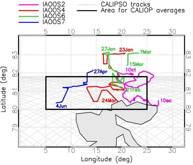
Measurements north of Svalbard were performed by the IAOOS2 system during the Barneo campaign between October and December 2014. IAOOS2 drifted from the north Pole (Barneo station) and reached the study region at the end of 2014. IAOOS4, IAOOS6, and IAOOS7 systems were deployed during the N-ICE2015 field experiment in January‒June 2015 [Granskog et al., 2016]. The numbering of the buoys #2 to #7 reflects their subsequent deployment in the Arctic. IAOOS2, IAOOS4, and IAOOS7 are NPBL systems, while IAOOS6 is a PBL. The drift path for the four buoys is shown in Fig. 1 and covers the region ~80-83°N latitude and ~7-27°E longitude.
2.3 The FLEXTRA model
The Lagrangian trajectory model FLEXTRA (FLEXible TRAjectories, Stohl et al., 1998) was used to track the origin and transport pathways of air masses. Seven‒days three‒dimensional backward and forward trajectories were calculated using as meteorological input either the ERA‒Interim reanalysis [Dee et al., 2011] or the ECMWF (European Centre for Medium-Range Weather Forecasts) operational analysis product. The model specific humidity and potential vorticity were interpolated along the trajectory path. The FLEXTRA model, being a trajectory model, does not take into account in its scheme aerosol dry and wet deposition, as it is done in dispersion models and in the recently released FLEXPART v10 (FLEXible PARTicle dispersion model; Grythe et al. [2017]). The lack of a dry and wet deposition scheme in FLEXTRA would possibly lead to an overestimation of the role of mid-latitude aerosol sources for aged air masses, while transport pathways may be increased by this lack of information. The statistical analysis of air mass origin and evolution presented in Sect. 4.3 then provides an upper limit of the contribution of mid-latitude aerosol sources. 3. Data analysis
3.1 CALIOP aerosol statistics in the 80-81.8°N 5-25°E region
CALIOP data in the 80-81.8°N 5-25°E region (Fig. 1) for the period October 2014 to June 2015 were used to build up a statistics of aerosol observation north of Svalbard. Data were available for the entire period with the exception of 10 days at the end of June. Aerosol observations from CALIOP were considered for subsequent analysis if the following requirements were met: (i) the aerosol optical depth (AOD) at 532 nm for each single aerosol layer is between 0.005 and 1; (ii) the feature type quality assessment (QA) is 2 or 3, i.e. medium or high confidence level in aerosol identification; and (iii) the aerosol layer is deeper than 200 m height. Given these conditions, the number of CALIOP observations was ~200
for each day in the considered region. Starting from the selected observations the following quantities were derived as daily averages:
- the aerosol occurrence (%) estimated as the ratio between the number of CALIPSO pixels with at least one aerosol layer in the column and the total number of CALIPSO pixels in the region. The aerosol occurrence was calculated for the whole 0-10 km altitude range and separately at 0-2, 2-5, and 5-10 km. The percent contribution by each aerosol subtype to the total occurrence was also estimated;
- the column‒equivalent daily extinction coefficient (Extinctioncolumn‒eq), that is the
average columnar extinction over the region. To calculate it first the total number of aerosol layers (Ntot), the total AOD (AODtot), and the total aerosol depth in km (Δztot) were
calculated by summing over all the detected aerosol layers between 0 and 10 km over the whole region. Then, the daily total extinction coefficient (Extinctiontot) was calculated as
1
tot tot tot AOD Extinction Mm 1000 z (km) (1).The daily column‒equivalent extinction coefficient was then estimated as
tot column eq mean tot Extinction Extinction N N (2)
with Nmean the average number of aerosol layers for each profile in the region for the
considered day. The uncertainty on Extinctioncolumn‒eq was estimated to be ~40% following
the uncertainty on the AOD reported by Winker et al. [2009]. These data will be presented and discussed in Sect. 4.2 and 4.3. 3.2 IAOOS local‒scale feature identification
Measurements from the IAOOS lidars were processed to identify the presence of aerosols and clouds from ground‒based local observations. Results are reported in Sect. 4.4. Raw data were analyzed following Mariage et al. [2017] to obtain the attenuated backscatter ratio vertical profiles (SRatt (z)):
p 2 att p m (z) SR z 1 T (z) (z) (3)In Eq. (3) βm(z) and βp(z) are the respective backscattering signals by molecules and particles,
while T (z)p2 is the two-way transmissions by particles (see Appendix A). The obtained SRatt
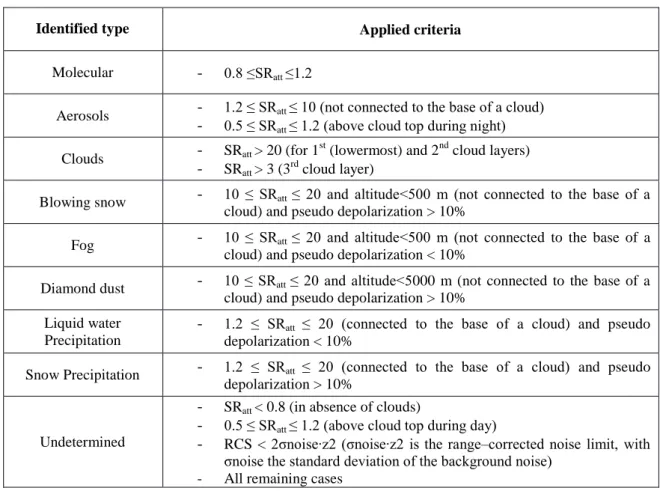
profile between 100 m and 8000 m was used to classify different type of observations by following an approach similar to that used for CALIOP observations [Vaughan et al., 2005, 2009]. Conditions listed in Table A1 in the Appendix were used to identify the presence of a specific feature in the profile based on SRatt data. The different identified categories are: 1.
molecular, corresponding to a clear profile; 2. aerosols; 3. clouds; 4. blowing snow/fog/DD; 5. precipitation; 6. undetermined. Diamond dust (low concentration of ice crystals) is slowly precipitating crystals occurring at low temperature in clear air [Curry et al., 1990]. Such crystals were frequently observed in winter near the surface [Intrieri and Shupe, 2004], but
they may be formed in altitude without any cloud formation when conditions are met [Girard and Blanchet, 2001]. Precipitating ice clouds may correspond to larger optical depths (and scattering ratios) but its identification may be difficult from the surface. Diamond dust can be differentiated from blowing snow from their smaller optical depth and possible larger vertical extent. Diamond dust (or blowing snow) and fog (water droplets) can be separated when depolarization information is available.
Once identified the presence of a specific feature then its apparent base and top altitude were determined by looking at the absolute value and variability of SRatt. For identified aerosol (or
cloud) layers the integrated attenuated backscatter (IAB) between the top and the bottom of the layer was calculated from SRatt by using the following formulas [Vaughan et al., 2005]:
att m
bottom
k 1 k k 1 k
k top 1
top bottom top bottom
A SR (z) (z) 1 B (z z ) (A A ) 2 1 IAB B (z z ) (A A ) 2
(4)When clear air can be detected above aerosol, haze or semi-transparent cloud layers from an extended region with SRatt values smaller than 1, an estimate of the optical depth and lidar
ratio can be given [de Villiers et al., 2010]. For the IAOOS6 polarized system the pseudo depolarization (δ) profile (defined as the ratio of the total perpendicular‒ to total parallel‒polarized backscattering signals (see Appendix A)) was also calculated.
3.3 Direct comparison of CALIOP and IAOOS and analysis along air mass trajectories: challenges and strategy
One of the objectives of the paper, as presented in Sect. 4.5, is to directly compare CALIOP and IAOOS observations and combine observations with FLEXTRA trajectories in order to investigate the capacity of the space‒borne lidar to (i) correctly classify aerosol subtypes and to (ii) detect and follow aerosol plumes to and from the Arctic. This type of comparison may be challenging, in particular due to the little spatial overlap between CALIOP and IAOOS, and the different temporal resolution of the two instruments. In order to provide a robust analysis, the following procedure derived from previous studies [De Villiers et al., 2010; Ancellet et al., 2016] was applied. First, for all IAOOS identified aerosol events the seven‒days backward and forward air mass trajectories were calculated with the FLEXTRA model. CALIOP traces falling within a circle of 100 km and ± 3h from each backward and forward trajectory points from FLEXTRA (1 per hour) were selected. For these selected traces CALIOP data fulfilling the requirements discussed in Sect. 3.1 (AOD at 532 nm between 0.005 and 1, feature type QA≥ 2, and aerosol layer thickness > 200 m) and falling (i) within ±25 km from the closest point of the trace to the trajectory calculated with FLEXTRA and (ii) less than 0.5 km away from the air mass altitude, were considered. This CALIOP subset was considered and the aerosol, cloud, and clear sky occurrence in it was calculated. The CALIOP subset was classified as aerosol‒, cloud‒, or clear-sky‒dominated if the respective occurrence of these features was >50%, otherwise the subset was classified as undetermined. For cases with an aerosol occurrence larger than 10% the average and standard
deviation of the IAB at 532 nm, of the pseudo Color ratio (CR*, see Appendix A), and of the pseudo depolarization ratio (δ) were estimated. CALIOP data were compared to IAOOS observations close to the buoy position and analyzed along air mass trajectories.
CALIOP and IAOOS operate at different wavelengths (532 and 1064 nm for CALIOP and 800 nm for IAOOS). This wavelength difference may affect the feature identification for the two instruments, as the attenuated scattering ratio is depending on molecular backscattering strongly varying with wavelength ( as-4, whereas particle backscattering is much less varying (~-4 to 0 with increasing particle size), and so the quality and significance of comparison concerning aerosol or cloud detection close to the buoys position. The pseudo depolarization ratio, also compared between CALIOP and IAOOS, shows a spectral variability (see Burton et al. [2015]), but its wavelength dependence is rather weak compared to the differences between pollution or marine aerosol and diamond dust types. The largest spectral dependence of δ was reported for smoke aerosol, for which 800 nm depolarization is less than 2% while it can be between 5% and 10 % at 532 nm. Wavelength differences were taken into account for the Lidar Ratio, with the values at 800 nm obtained from IAOOS reported at 532 nm following Cattrall et al. [2005] for comparison with CALIOP observations.
4. Results and discussion 4.1 Meteorological conditions
ERA-Interim gridded data (0.75° latitude by 0.75° longitude) were used to analyze transport of air masses and their meteorological characteristics. Averages of 2-m temperature (T2m), mean sea level pressure (MSLP), wind speed and wind direction over the 80-81.8°N and 5-25°E region for the period October 2014 to June 2015 are reported in Fig. S1. The surface temperature varied between about 0 and -30°C during autumn and winter and raised stably to 0°C at the beginning of June. The MSLP was very variable in late autumn and winter and more stable in spring and summer. In winter the MSLP drops corresponded usually to T2m and wind speed increases which indicate the occurrence of synoptic‒scale storm events. Three major polar lows occurred over the domain in January and February, leading to 30°C increase in the surface temperature and strong south-westerly flows.
The wind direction was very variable in all seasons but depending on average prevailing synoptic conditions. The wind speed and direction distribution for the different seasons (autumn, October to December (OND); winter, December to March (DFM); spring-summer, April to June (AMJ), Fig. S2) suggests the dominance of southerly winds in OND. These were due to the strong cyclone activity in the North Atlantic and Northern Europe in this period (see Fig. S3 for seasonal geopotential map anomalies). In JFM the winds were predominantly from the east and south-east direction, corresponding with the northward shift of the low pressure systems caused by the unusual position of the polar vortex, with a marked pressure dipole structure over eastern Alaska and eastern-Siberia and higher pressure over western Russia [Cohen et al., 2017]. The circulation completely changed during AMJ due to the disappearance of the polar vortex and the shift of the low pressure over Scandinavia which favored the occurrence of more northerly winds. Also, the shift to an Arctic Dipole
pattern (i.e., lower pressures over western Artic and higher pressure over eastern Arctic) in May and June contributed to the instauration of the northerly regime.
Our observations obtained over a larger domain are in relative good agreement with local meteorological data obtained during the N-ICE2015 campaign [Cohen et al., 2017].
The November 2014 to June 2015 period was also characterized by a positive phase of the North Atlantic Oscillation (NAO), which indicates favorable large scale meteorological patterns for air pollution transport towards the Arctic [Eckhardt et al., 2003], as well as strong El Niňo conditions (Oceanic Niňo Index, ONI, between 0.5 and 1), estimated to induce a stronger impact of Asian source to the Arctic [Fisher et al., 2010].
4.2 Aerosol occurrence, type, and optical properties in the high Arctic from CALIOP observations
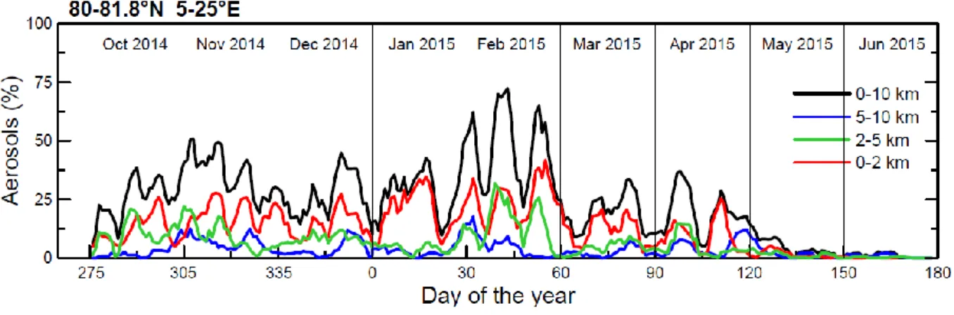
The temporal evolution of the vertical‒resolved aerosol occurrence over the 80-81.8°N 5-25°E region from CALIOP data is shown in Fig. 2. The total aerosol occurrence between 0 and 10 km was relatively large (>25%) between October and February, moderate (10-30%) in March and April, and very low (<5%) in May and June, in agreement with the seasonal cycle of aerosol mass obtained at Ny‒Ǻlesund (Svalbard) by Tunved et al. [2013]. Absolute maxima were measured in February (~75%). The mean (standard deviation) of the aerosol occurrence over the entire period was 23% (±22%). The cloud occurrence from CALIOP data over the same period (not shown) was between about 15 and 95%, with an average of 61% (±32). Aerosols were mostly confined below 2 km (50% of observations on average), followed by particles in the 2-5 km (31%) and 5-10 km (19%) altitude ranges. End of January to the end of February is the period showing the largest occurrence of aerosols. A secondary peak is also seen in November.
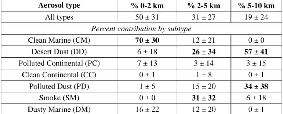
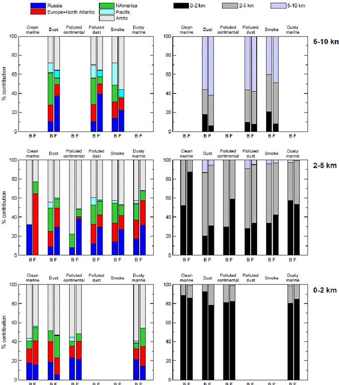
The contribution by the different subtypes to the total aerosol load and extinction varies with altitude as indicated in Table 1 and Fig. 3. Below 2 km the aerosol load was dominated by the clean marine type (70% of observations on average) and dusty marine (16%), with lower contributions by polluted continental (7%) and desert dust (6%). Extinction was in the range 1-8 Mm-1 below 2 km (4.5 ± 2.0, mean and standard deviation) and was mostly attributed to clean marine aerosols in OND, in link with the southerly wind regime during this period, and to dusty marine and desert dust types in JFM. In the 2-5 km range the aerosol load was dominated by smoke (31%) and desert dust (26%) subtypes, with minor contributions by polluted dust (15%), clean marine (12%), and dusty marine (12%) types. Extinction at 2‒5 km varied in the range 1-18 Mm-1
(6.5 ± 4.8, mean and standard deviation), with a strong peak in October‒January and a second peak in March. At 5‒10 km aerosols were in large majority classified as dust (57%) and polluted dust (34%), with an associated small and almost constant extinction (0-6 Mm-1; 2.1 ± 1.4, mean and standard deviation). The clean continental subtype had a negligible contribution at all altitudes. The extinction coefficient did not show a clear seasonal cycle at 0‒2 km and 5‒10 km altitude ranges, while at 2‒5 km it showed a more marked seasonal variation with larger values in autumn/winter and lower values towards spring and summer. The estimated columnar‒equivalent AOD at 532 nm was in the range 0.0002-0.003 (0‒2 km), 0.0001-0.004 (2‒5 km), and 0.0001-0.001 (5‒10 km).
Figure 3 shows extinction data also for an additional class which corresponds to the whole dataset minus dust-type observations (dust, polluted dust, and dusty marine). As discussed later in the paper, we argue that these subtypes can be in part DD or icy clouds misclassified as aerosols in the CALIPSO algorithm. Data for this class, providing a lower limit of extinction for aerosols not contaminated by DD or clouds, are in the range 1-8 Mm-1 (0‒2 km), 1-14 Mm-1 (2‒5 km), and 0-2 Mm-1 (5‒10 km).
Aerosol occurrence, subtype classification, and optical properties were also analyzed around our main area of investigation (six sub‒regions of latitude 75, 78, 81.8°N and longitude 5, 15, 25°E). Results indicate a relative spatial homogeneity of aerosol extinction and repartition of different subtypes in the different altitude ranges compared to the 80-81.8°N 5-25°E region. Exceptions were in May and June, with larger extinctions measured in the eastern part (15-25°E) in late May and in the south-eastern sector (75‒78°N 15‒25°E) in June, possibly in relation to specific aerosol transport events.
4.3 Aerosol sources and fate in the high Arctic from CALIOP observations and FLEXTRA modelling
Seven‒days backward and forward trajectories were performed in order to understand the sources and fate of high Arctic aerosols. To this purpose, a trajectory per day was calculated with the FLEXTRA model for each aerosol subtype identified by CALIOP in the 80-81.8°N 5-25°E region. ERA‒I reanalysis were used as meteorological input to the model. The point of arrival/departure for the backward/forward trajectories was estimated as the centroid of the latitude, longitude, and altitude of the CALIOP observations for the subtype, while the time of arrival/depart was set commonly for all subtypes at the average time of CALIOP aerosol observations for the day. Only aerosol subtypes with a statistically significant number of observations were considered for trajectory analysis. These were clean marine (127 cases), desert dust (111), polluted continental (48), polluted dust (103), smoke (112), and dusty marine (78). All obtained trajectories are shown in Fig. S4‒S9.
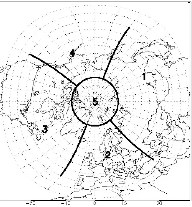
A statistical analysis was performed on obtained trajectories. We defined five areas in the northern hemisphere (Russia, Europe/North Atlantic, North America, Pacific, and Arctic, Fig. 4) and we calculated the percent of time spent by each trajectory over each area, as well as the percent of time that each trajectory spent at different altitude ranges along its path.
As discussed in Sect. 4.2, dusty marine, dust and polluted dust subtypes were observed to contribute significantly to extinction both in the lower troposphere below 2 km and in the 2‒5 km middle tropospheric layers. These types are identified as they are linked to a significant depolarization ratio [Omar et al., 2009, Vaughan et al., 2017]. The analysis of backward trajectories however raises doubts on the dusty origin of particles for these observations. Wintertime dust and polluted dust (Fig. 5, JFM) show a preferential pattern of transport from North America (in areas mostly covered by snow) and the Atlantic Ocean, while dusty marine corresponds to trajectories originated in the close surrounding of the Arctic Ocean then spending about 60% of the time over the sea, and staying in the vicinity of snow‒covered land. The trajectories for dust, polluted dust and dusty marine cases also indicate air masses rich of moisture for which cloud formation would be favored in the Arctic. In particular, observations for dust corresponded to very high CALIOP estimated
pseudo depolarization ratios (up to 0.6), which would suggest that these observations better corresponds to ice particles showing much larger depolarization than aerosols [Burton et al., 2012]. Only during the spring to summertime period (AMJ) a small fraction of dust and polluted dust trajectories above 2 km showed trajectories possibly corresponding to dust transport from desert sources in East Asia (from latitudes lower than 45‒50°N where the Gobi and Taklimakan deserts are found). These were identified as sources of dust for the Arctic via different previously identified long‒range pathways [e.g., Huang et al., 2015]. A fraction of trajectories at 2‒5 and 5‒10 km also came from Southern Europe, a possible source of dust aerosols originating from the close Sahara desert. As mentioned before, taking into account dry/wet deposition, may somehow limit the number of trajectories reaching these sources.
Figure 6 shows the results of the statistical trajectory analysis separately for each aerosol subtype and for the 0‒2, 2‒5, and 5‒10 km altitude ranges. Trajectories arriving in the high Arctic (left panel of Fig. 6, bars labelled as B) were for the ~30‒40% from the Russia and Europe/North Atlantic sectors. This was observed independently of the aerosol subtype including the clean marine type. For clean marine however we would not expect an Eurasian origin, and the fact of having a significant fraction of trajectories from this sector could be an indication that the clean marine type below 2 km in the Arctic is contaminated by pollution particles. The contribution of North American sources increased with altitude for all aerosol subtypes except clean marine (<10% at 0‒2 km and 15‒35% at 2‒5 and 5‒10 km). In particular, a clear contribution of Northeastern American sources was obtained for smoke at 2‒5 km (Fig. S8). Stohl et al. [2006] also found significant winter and spring transport from Eurasia with less transport from North America. This feature is emphasized during the positive phase of the NAO [Eckhard et al. 2003]. During the ARCTAS-A campaign (April-June 2008), the North American contribution was however more important especially for the pressure altitude above 700 hPa, in good agreement with our analysis. The Pacific area contributed significantly (11‒24%) only at 5‒10 km altitude and less than 7% and 4% at 2‒5 and 0‒2 km, respectively. For all aerosol subtypes, a significant portion of time (40‒80%, i.e. 3 to 6 days) was spent by trajectories in the Arctic region; this contribution decreases to ~30% (~2 days) at 5‒10 km indicating trajectories more rapidly crossing the Arctic. This is in agreement with results by Stohl [2006] who found that the time spent by air masses in the Arctic was about 1 week in winter in the lower and middle‒troposphere and about 3 days in the upper layers. Several studies, based both on trajectories analyses [Stohl, 2006; Rozwadowska et al., 2010; Hirdman et al., 2010; Fuelberg et al., 2010; Fisher et al., 2010; Matsui et al., 2011] and regional chemical transport models [Klonecki et al., 2003], have analysed the patterns of aerosol transport into the Arctic. Most of these studies confirm the previous description, as they show that Europe and Central and Eastern Siberia contribute to the aerosol content in the lower troposphere, while transport from North America and eastern Asia mostly affects higher levels. A large spread exists in evaluating the potential contribution of different source regions to the Arctic aerosols and distribution, where these discrepancies are mainly related to the different representations of removal mechanisms and photochemical reactions in models [Shindell et al., 2008].
Forward trajectories (left panel of Fig. 6, bars labelled as F) suggest that at 0‒2 km the air masses, which mostly originated in Russia and Europe/North Atlantic, mostly came back to Russia and Europe/North Atlantic (23‒41%), but also partly went towards North America (8‒24%). On the contrary, at both 2‒5 and 5‒10 km ranges, the trajectories which originated in Russia and Europe/North Atlantic, but in part also in North America and Pacific sectors, predominantly travelled towards Russia and Europe/North Atlantic (42‒65% at 2‒5 km and 36‒50% at 5‒10 km). Only a minor part of trajectories above 2 km came back to North America and the Pacific (<7% and <8% at 2‒5 km and <14% and <1% at 5‒10 km, respectively). The residence time in the Arctic was also significant in the forward direction (44-53% (~3.50 days) at 0-2 km, 23-51% (~1.5‒3 days) at 2-5 km, and 36-56% (~2.5‒4 days) at 5-10 km).
Concerning altitude (right panel of Fig. 6), air masses arriving at 0‒2 km remained confined well below 2 km most of the time both along their backward and forward trajectories (>78%), in very few cases overpassing 5 km altitudes (<1%). Air masses arriving at 2‒5 km also remained below 5 km along their backward and forward path (20‒57% at 0‒2 km and 40‒70% at 2‒5 km in backward and 31‒87% at 0‒2 km and 13‒64% at 2‒5 km in forward), with less than 13% (backward) and 6% (forward) contributions at 5‒10 km. Finally, trajectories arriving at 5‒10 km remained most of the time in this altitude range (40‒56% in backward and 49‒62% in forward), descending only in some cases at 2‒5 km (26‒40% in backward and 32‒43% in forward) and 0‒2 km (10‒21% in backward and 6‒8% in forward). These observations indicate very low vertical mixing.
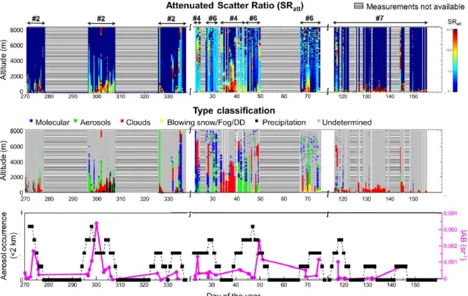
4.4 Local‒scale IAOOS observations north of Svalbard during October 2014‒June 2015 Figure 7 shows the vertical cross section of the attenuated backscatter ratio at 800 nm, feature classification, and occurrence and IAB of aerosol layers below 2 km measured by the four IAOOS lidars between October 2014 and June 2015 north of Svalbard. Ground‒based lidar data indicate a high frequency of aerosol occurrence in October/early November (days 270‒280 and 295‒310), December (days 320‒355), January‒February (days 27‒50), March (days 65‒75), and April (days 115‒121), in agreement with CALIOP observations in the region. Aerosols were mostly confined below about 2 km altitude, with some cases in February and March extending up to 5‒6 km. From 2nd to 9th February (days 33‒41) a low pressure system affected the area and deep clouds from the ground to ~4 km were detected. Clouds, and in particular low‒level clouds with bases usually below 500 m, dominated observations at the end of October (days 300‒305) and between late April and June (days 117‒156). Few cases of blowing snow/fog/DD were also detected, in particular during winter months.
As indicated in Fig. 7 IAOOS lidar measurements were not available in several periods. This was due primarily to the icing of the lidar window between October and March, while in the April to June period this was due to the frequent occurrence of very low and thick cloud layers which completely saturated the signal.
4.5 Case studies: identification of aerosol transport to the high Arctic with IAOOS/CALIOP observations and FLEXTRA modelling
For all IAOOS identified aerosol events in Fig. 7 we calculated the seven‒days backward and forward air mass trajectories with the FLEXTRA model run with the ECMWF operational analysis. We chose the ECMWF dataset this time given its higher resolution, most adapted to investigate the air mass dynamics in link to local scale observations. These trajectories indicate, as some cases reported in Fig. 8, that aerosols mostly originated from Russia (central and eastern Siberia), with some air masses also from the central and Canadian Arctic and the Europe/North Atlantic sector, in agreement with the previous analysis.
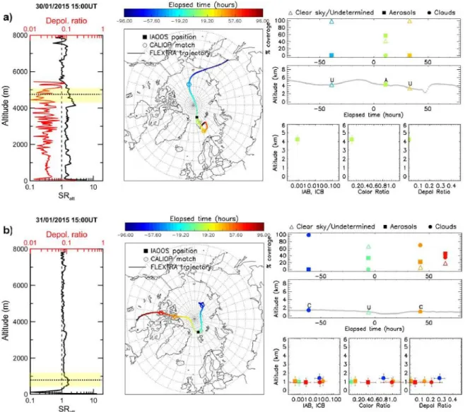
The data selection procedure and analysis described in Section 3.3 was applied to analyze CALIOP observations in link to IAOOS data. Examples of combined IAOOS, CALIOP, and FLEXTRA data are shown in Fig. 8 for cases corresponding to observations taken the 30th and 31st January (Fig. 8a), 14th (Fig. 8b) and 18th February 2015 (Fig. 8c). Data for the 30th January and 14th and 18th February are from the IAOOS6 system measuring the two polarizations and so allowing obtaining pseudo depolarization profiles; conversely, 31st January data are from the IAOOS4 non‒depolarizing system.
The aerosol load measured by IAOOS at 800 nm was very low on January 31st (total columnar IAB~7.3 10-4 sr-1), while larger values were observed on January 30th (IAB~6.4 10
-3
sr-1), and February 14th (IAB~7.3 10-3 sr-1) and 18th (IAB~3.5 10-3 sr-1). For the case of February 14th, CALIOP was able to clearly identify the presence of aerosols both along backward and forward trajectories and in proximity of the IAOOS position. In contrast, for January 30th and 31st and February 18th, CALIOP identified the presence of aerosols close to the IAOOS position but not in the backward trajectories, and only in part in the forward trajectories. The analysis of all identified IAOOS aerosol events indicate that CALIOP is only able in ~30% of cases to identify the presence of aerosols in proximity of the IAOOS position and that most part of these layers have an IAB ≥ 0.001 sr-1
at 800 nm (over 1 km altitude extent). These observations confirm the threshold identified for CALIOP measured IAB at 532 nm allowing efficient aerosol detection at ~1 10-3 km-1sr-1 [Winker et al., 2009].
The CALIOP algorithm classified aerosol observations in Fig. 8 as smoke on January 30th and 31st, while for February 14th the dominant subtypes were dusty marine at 1000 m and polluted dust at 3000 m. The rather low measured CALIOP pseudo color ratio (CR*~0.1) and large backscatter ratio (SRatt>2) for the case of 14th February however would suggest small
particles, but rather high depolarization ratios are indicative of the presence of non‒spherical particles. Assuming that clear air is observed on the IAOOS profile for February 14th above 5 km, over an extended range of altitude where SRatt is almost constant, one can determine that
the two-way transmission loss due to particle scattering and absorption is about 60%, which corresponds to an AOD value of ~0.25 at 800 nm. The IAB of 7.3 10-3 sr-1 retrieved for the February 14th IAOOS profile combined with the measured transmission allow to estimate for the aerosol layer between 0 and 5 km an average IAOOS lidar ratio (LR) of 27(±6) sr at 800 nm, considering measurement uncertainties of ±10% for both transmission and IAB, and multiple scattering correction [Mariage et al., 2017]. It corresponds to a 532-nm lidar ratio of 29(±8) sr assuming the spectral dependence proposed by Cattrall et al. [2005]. This value
better corresponds to ice clouds (LR~25-30 sr at 532 nm) [Garnier et al., 2015] possibly including clean continental particles (LR~35 sr) than pure desert dust (~45-55 sr), polluted dust or polluted particles/smoke and arctic haze having much larger LR values [Omar et al., 2009; Burton et al., 2012].
For the case of February 18th clean marine aerosols were identified by CALIOP below 1200 m and dusty marine near the surface, both originating from industrial areas in north-west Russia. A cirrus cloud was detected at 5-6 km. For this day, depolarization measurements were also available from IAOOS lidar. The IAOOS observed profile was similar to the CALIOP one, with the presence of an ice cloud between 5 and 6 km (volume pseudo depolarization ratio about 30%), and two layers below 1200 m, one very weakly depolarizing at 800 nm (2-3 % from 200 to 1200 m) for an average attenuated backscatter ratio of about 5 at 800 nm, and the lowermost one (below 200 m) more depolarizing (about 20% at 800 nm), and more scattering (SRatt~40). A total IAB of 3.5 10-3 sr-1 was retrieved by
IAOOS for the whole layer up to 1200m. Combining IAB and transmission measurements (T2~60%) allowed to estimate for these aerosols an averaged LR of 58(±12) sr at 800 nm. It corresponds to a 532-nm lidar ratio of 77(±19) sr i.e. a value better corresponding to pollution aerosols (LR~70 sr at 532 nm) than marine particles (LR~20 sr) [Omar et al., 2009]. Assuming the lower layer is attributed to diamond dust or more likely to blowing snow, as this corresponds to an observed strong wind event [Cohen et al., 2017], with LR ~30 sr, leads to a lidar ratio larger than 60 sr for the layer above. Such discrepancies have been observed in previous comparisons, as CALIOP algorithm is preferentially selecting clean marine than polluted continental near the surface away from land over the ocean, leading to lower lidar ratios and consequently bias low their AODs [Rogers et al., 2014]. IASI (Infrared Atmospheric Sounder Interferometer) data (not shown) indicate that trajectories arriving at the IAOOS position between 500 and 1000 m during this day crossed a region in north‒west Russia where high carbon monoxide concentrations (CO>3˟1018 molecules cm-2) were measured, thus corroborating the hypothesis of polluted particles transported to the Arctic. 5. Summary and Conclusions
We have presented measurements of the occurrence, properties, and vertical distribution of tropospheric aerosols as obtained from V4 CALIOP space‒borne and IAOOS ground‒based lidar observations in the high Arctic north of Svalbard in the period October 2014 to June 2015, and combined observations with FLEXTRA trajectory analysis.
CALIOP observations indicate a maximum in aerosol occurrence at the end of winter over the region attributed to low‒level (0-2 km) and mid‒tropospheric (2-5 km) particles. Another maximum was observed in October‒December. The CALIOP aerosol extinction coefficient at 532 nm was in the range 1-8 Mm-1 (0‒2 km), 1-18 Mm-1 (2‒5 km), and 0-6 Mm-1 (5‒10 km), with largest values in the October‒December period. Mean values (± standard deviation) are 4.5 (±2.0) Mm-1 at 0‒2 km, 6.5 (±4.8) Mm-1 at 2‒5 km, and 2.1 (±1.4) Mm-1 at 5‒10 km. Aerosol extinctions as obtained in this study from V4 CALIOP are smaller (up to a factor 2) than those obtained by Di Pierro et al. [2013] using V3 data and considering a larger Arctic domain. For instance, in the Eurasian Arctic (69-82° N and 10-110° E) they found an extinction of ~5‒22 Mm-1
showing a pronounced seasonal cycle with maxima in winter and minima in summer. Our data, in contrast, do not show any marked seasonality in the total extinction signal below 2 km, but they show it the 2‒5 km range. Only the identified clean marine aerosol subtype shows seasonality below 2 km with maxima in the October‒December period, in agreement with long‒term observations in the Svalbard [Huang et al., 2017].
The analysis of backward trajectories indicates that below 2 km aerosols originate mostly from Russia and Europe, while above 2 km significant sources are also North America and the Pacific areas. Air masses have a significant residence time in the Arctic region (few days to about one week), after which they exit this region. Aerosols below 2 km altitude are estimated in large part to come back to their source areas in Russia/Europe, but also in part to be transported towards North America. In contrast, above 2 km, aerosols which are originated in Russia/Europe and North America/Pacific sectors, are transported mostly towards Russia and Europe. The combination of backward and forward trajectories shows therefore that the Arctic is a pathway for aerosols exchange and crossing from Russia/Europe to North America (below 2 km) and from North America to Russia/Europe (above 2 km). These observations suggest different considerations. First, Russia and Europe are both sources, but also sinks for high Arctic low‒tropospheric aerosols. Second, North America is a source for mid‒ and high‒altitude aerosols and in part a sink for low‒tropospheric particles.
Based on our observations, in agreement with De Villiers et al. [2010] and Law et al. [2014], we confirm that transport from Asia to Europe and North America through the Arctic are pathways for pollution that could affect air quality, cloud formation, and radiative balance in these regions. On the other hand, the Arctic also favours the inverse pathway, with aerosols transported from North America to Russia and Europe. This however is observed at altitudes higher than 2 km, where aerosol concentrations are expected to be smaller, and the export mostly associated to episodic events. Anyhow, reinforcing the economic policy focused on carbon‒burning activities is expected in the next years to induce a strong increase of North American emissions which, along with increasing wildfire emissions, would enhance aerosol-induced impact on Arctic (Law et al., 2014, Zamora et al., 2016).
Ground‒based IAOOS lidar observations north of Svalbard enabled the identification of small scale aerosol features. The analysis of case studies suggests that when the aerosol layers are relatively optically thick (backscatter coefficient B≥0.001 km-1sr-1) CALIOP is able to efficiently detect them and to follow their transport to and from the Arctic. Henceforth, in such cases, CALIOP data could be considered as a valuable source to retrieve information on aerosol aging. Instead, for optically thinner layers (B<0.001 km-1sr-1) CALIOP proves relatively efficient in detecting aerosols in correspondence of the IAOOS position, but is not able to fully characterize the transport and evolution of the plumes. These observations suggest in general the good CALIOP sensitivity to the presence of both thin and thick aerosol layers during nighttime. On the other hand, they put in evidence the limitations in the FLEXTRA/CALIOP synergy to identify aerosol origin and evolution, in particular for the very low aerosol loads in the high Arctic.
A significant fraction of high Arctic aerosol observations both in the low‒troposphere and in the upper layers were classified as dust-type (desert dust, polluted dust, and dusty
marine) in the CALIOP identification‒type algorithm, owing to their high depolarization ratio and rather low backscattering coefficient. Dust‒type is corresponding to irregularly shaped and large sized particles, and no other depolarizing particle type specific to Arctic has yet been introduced in the CALIOP classification. Looking to back-trajectories, no significant potential sources of mineral particles were identified, especially in wintertime. We found, instead, that dust and polluted dust observations have mostly a common pattern corresponding to trajectories from North America and the Atlantic Ocean, while dusty marine are mostly related to local scale circulation patterns. In both cases trajectories suggest air masses with high moisture contents and low temperatures for which diamond dust or ice cloud formation can be favored in interaction with aerosols. By combining CALIOP dust‒type observations with co‒located local‒scale aerosol IAOOS measurements on a few case studies we also found additional indication that low-level dust‒type observations could be more likely associated to blowing snow, diamond dust or tiny ice clouds occurring not only near the surface, as expected from previous observations, but also in the mid troposphere.
CALIOP also identified a dominant fraction of lower‒tropospheric aerosols as clean marine type. Back‒trajectories indicate that such aerosols were staying several days over the Arctic but however mostly originated in Russia and Europe, and would thus more likely correspond to polluted aerosol types. The analysis of a few co‒located IAOOS profiles corroborates this hypothesis, suggesting the possible underestimation of the polluted‒type aerosols in the CALIOP retrievals over the Arctic.
The merging of satellite data with local‒scale observations and trajectories analysis can improve the CALIOP type identification, in particular in regions where ice clouds or diamond dust could be present and where long‒range transport plays a dominant role. More detailed analyses over larger temporal and spatial scales of aerosol properties and identification procedures should further allow better clarifying and using CALIOP aerosol information in the Arctic region. In particular, a further key step should also include the comparison of remote sensing data with in situ airborne observations, which would help the identification and discrimination of different atmospheric features (clouds/aerosols/diamond dust) and better characterize cloud‒aerosol interactions. This should be part of the objectives of future Arctic field experiments, as for instance discussed in the forthcoming international MOSAIC project (Multidisciplinary drifting Observatory for the Study of Arctic Climate, http://www.mosaicobservatory.org/) that will provide extensive in situ and remote sensing observations in the Arctic atmosphere.
Appendix Appendix A
In this appendix we define the attenuated backscatter ratio (SRatt), particle depolarization
ratio, pseudo depolarization ratio (δ), color ratio (CR), pseudo color ratio (CR*), and lidar ratio (LR) and how these parameters are retrieved from backscatter lidar measurements. Starting from the measured raw lidar signal (S), the range corrected signal (RCS) is calculated as RCS=(S-N)*z2, with N the background signal noise and z the distance from the
lidar emitter. The RCS signal is related to the optical properties of atmospheric aerosols and molecules through the following formula:
2 2m p m p
RCS(z)
(z) (z) T (z) T (z)
O(z) C (A1)
The different terms in Eq. A1 are: the overlap function (O(z)) used to correct the signal below its overlap range; the system constant C; the backscattering signal of molecules βm(z) and
particles βp(z); and the two‒way transmission by molecules 2 m
T (z) and particlesT (z)p2 . The (molecular and particular) two‒way transmission is related to the optical depth (AOD) and the extinction coefficient (α(z)) by the following formula:
z
2
0
T (z)exp 2AOD exp 2
(z ')dz ' (A2)The attenuated backscatter ratio (SRatt) is derived by dividing the attenuated backscattering
given by expression A1 and the molecular signal m mT2 which can be estimated from climatological meteorological profiles so that
p 2 att 2 p m m m (z) RCS(z) SR (z) 1 T (z) O(z) C (z) T (z) (z) (A3).
When the aerosol attenuation is low, as it is frequently the case, we can assume that T (z)p2 ~1, and the attenuated ratio can be expressed as:
p att m (z) SR (z) 1 (z) (A4)
If the lidar uses a linearly polarized laser emission, then both parallel‒ and perpendicular‒polarized backscattered signals can be measured. The backscatter ratios for perpendicular- and parallel-polarized light are defined as:
p att m (z) SR (z) 1 (z)
,p att ,m (z) SR (z) 1 (z) (A5)and the ratio of the aerosol particle perpendicular- to parallel-polarized backscatter signals is the linear particle depolarization ratio:
att
,p p m ,p att SR (z) 1 (z) (z) (z) SR (z) 1 with ,m m ,m (z) (z) (z) (A6).The particle depolarization ratio depends critically on the absolute accuracy of the backscatter ratio retrieval, so the pseudo depolarization ratio (δ), defined as the ratio of the total perpendicular‒ to the total parallel‒polarized backscatter signals, is frequently used:
att
m p
m
att att att
SR (z) (z) 1 (z) (z) 1 (z) SR (z) SR (z) SR (z) (A7)
(z) is also called volume depolarization ratio. The color ratio (CR) is defined as the ratio of the aerosol backscatter at 1064 nm to the aerosol backscatter at 532 nm:
att
p,1064 p,532 att SR (z) 1 (z) 1 CR(z) (z) SR (z) 1 16 (A8)where 1/16 is the ratio of the 1064-nm to the 532-nm molecular backscatter. Similarly to the depolarization ratio, the pseudo color ratio (CR*) can be estimated from the total backscatter coefficients as:
* att 532 att (z) 1 1 1 CR (z) CR(z) 1 (z) SR (z) 16 SR (z) (A9)Finally, the lidar ratio (LR) is the ratio of the extinction ( (z)) to backscatter aerosol (p(z))
coefficients.
Table A1. Criteria used to distinguish between different features in the IAOOS lidar profiles using SRatt at 800 nm. Some categories cannot be separated when depolarization is not
available.
Identified type Applied criteria
Molecular - 0.8 ≤SRatt ≤1.2
Aerosols - 1.2 ≤ SRatt ≤ 10 (not connected to the base of a cloud)
- 0.5 ≤ SRatt ≤ 1.2 (above cloud top during night)
Clouds - SRatt > 20 (for 1
st (lowermost) and 2nd cloud layers)
- SRatt > 3 (3 rd
cloud layer)
Blowing snow - 10 ≤ SRatt ≤ 20 and altitude<500 m (not connected to the base of a
cloud) and pseudo depolarization > 10%
Fog - 10 ≤ SRatt ≤ 20 and altitude<500 m (not connected to the base of a
cloud) and pseudo depolarization < 10%
Diamond dust - 10 ≤ SRatt ≤ 20 and altitude<5000 m (not connected to the base of a
cloud) and pseudo depolarization > 10% Liquid water
Precipitation
- 1.2 ≤ SRatt ≤ 20 (connected to the base of a cloud) and pseudo
depolarization < 10%
Snow Precipitation - 1.2 ≤ SRatt ≤ 20 (connected to the base of a cloud) and pseudo
depolarization > 10%
Undetermined
- SRatt < 0.8 (in absence of clouds)
- 0.5 ≤ SRatt ≤ 1.2 (above cloud top during day)
- RCS < 2σnoise∙z2 (σnoise∙z2 is the range‒corrected noise limit, with σnoise the standard deviation of the background noise)
Acknowledgements and data
This work was supported by funding from the ICE-ARC programme from the European Union 7th Framework Programme, grant number 603887, ICE-ARC contribution number 072. The IAOOS program has been funded by the Agence Nationale de la Recherche (ANR-10-EQPX-32-01) and has been developed in partnership with LOCEAN at UPMC.
We thank the DT/INSU/CNRS for the preparation of the buoys, deployment and survey. We would like to particularly thank M. Calzas and A. Guillot for their help during the first two periods of N-ICE2015, and N. Geyskens and F. Blouzon for the IAOOS 2 campaign deployment. We wish to thank the Norwegian Polar Institute (NPI) for help in the field experiment and discussions. NASA, CNES, the ICARE/AERIS and the LARC data centres are gratefully acknowledged for supplying the CALIPSO data. The FLEXTRA team (A. Stohl and co-workers) is acknowledged for providing and supporting the FLEXTRA code Helpful comments and suggestions from three anonymous reviewers are also acknowledged. IAOOS atmospheric data used in this paper are available upon request to the corresponding author and will be soon available in the AERIS Data Portal at https://www.aeris-data.fr/. CALIPSO data used in this study are available from NASA at https://eosweb.larc.nasa.gov/ and in France in the AERIS/ICARE Data Portal at http://www.icare.univ-lille1.fr/. The FLEXTRA trajectory model used in this study can be downloaded at https://folk.nilu.no/~andreas/flextra.html, and the ERA‒Interim reanalysis and the ECMWF operational analysis product can be retrieved at http://apps.ecmwf.int/.
References
Acosta Navarro, J. C., V. Varma, I. Riipinen, Ø. Seland, A. Kirkevåg, H. Struthers, T. Iversen, H.-C. Hansson, and A. M. L. Ekman (2016), Amplification of Arctic warming by past air pollution reductions in Europe, Nat. Geosci., 9, 277–281, doi:10.1038/ngeo2673.
Aliabadi, A. A., et al. (2016), Ship emissions measurement in the Arctic by plume intercepts of the Canadian Coast Guard icebreaker Amundsen from the Polar 6 aircraft platform, Atmos. Chem. Phys., 16, 7899-7916, doi:10.5194/acp-16-7899-2016.AMAP (2015). AMAP Assessment 2015, Black carbon and ozone as Arctic climate forcers. Arctic Monitoring and Assessment Programme (AMAP), Oslo, Norway, 116 pp.
Ancellet, G., J. Pelon, Y. Blanchard, B. Quennehen, A. Bazureau, K. S. Law, and A. Schwarzenboeck (2014), Transport of aerosol to the Arctic: analysis of CALIOP and French aircraft data during the spring 2008 POLARCAT campaign, Atmos. Chem. Phys., 14, 8235-8254, https://doi.org/10.5194/acp-14-8235-2014. Ancellet, G., J. Pelon, J. Totems, P. Chazette, A. Bazureau, M. Sicard, T. Di Iorio, F. Dulac, and M. Mallet
(2016), Long-range transport and mixing of aerosol sources during the 2013 North American biomass burning episode: analysis of multiple lidar observations in the western Mediterranean basin, Atmos. Chem. Phys., 16, 4725-4742, doi:10.5194/acp-16-4725-2016.
Becagli, S., L. Lazzara, C. Marchese, S. E. Ascanius, M. Cacciani, U. Dayan, C. Di Biagio, T. Di Iorio, A. di Sarra, P. Eriksen, F. Fani, D. Frosini, D. Meloni, G. Muscari, G. Pace, M. Severi, R. Traversi, and R. Udisti (2016), Relationships linking primary production, sea ice melting, and biogenic aerosol in the Arctic, Atmos. Environ., 136, 1-15, doi: 10.1016/j.atmosenv.2016.04.002.
Bourassa, M. A., et al. (2013), High-Latitude Ocean and Sea Ice Surface Fluxes challenges for Climate Research. B. Am. Meteor. Soc., 94, 403–423, doi:10.1175/BAMS-D-11-00244.1.
Brock, C. A., Cozic, J., Bahreini, R., Froyd, K. D., Middlebrook, A. M., McComiskey, A., Brioude, J., Cooper, O. R., Stohl, A., Aikin, K. C., de Gouw, J. A., Fahey, D. W., Ferrare, R. A., Gao, R.-S., Gore, W., Holloway, J. S., Hübler, G., Jefferson, A., Lack, D. A., Lance, S., Moore, R. H., Murphy, D. M., Nenes, A., Novelli, P. C., Nowak, J. B., Ogren, J. A., Peischl, J., Pierce, R. B., Pilewskie, P., Quinn, P. K., Ryerson, T. B., Schmidt, K. S., Schwarz, J. P., Sodemann, H., Spackman, J. R., Stark, H., Thomson, D. S., Thornberry, T., Veres, P., Watts, L. A., Warneke, C., and Wollny, A. G. (2011), Characteristics, sources, and transport of aerosols measured in spring 2008 during the aerosol, radiation, and cloud processes affecting Arctic Climate (ARCPAC) Project, Atmos. Chem. Phys., 11, 2423-2453, https://doi.org/10.5194/acp-11-2423-2011.
Blanchard Y., J. Pelon, E. Eloranta, K. PMoran, J. Delanoë, G. Sèze, A synergistic analysis of cloud cover and vertical distribution from A-Train and ground-based sensors over the high Arctic station EUREKA from 2006 to 2010, J. Atmos. Meteor. Climatol., 2014, 53 (11), pp.2553-2570. <10.1175/JAMC-D-14-0021.1>. Burton S., R. A. Ferrare, C. A. Hostetler, J. W. Hair, R. R. Rogers, M. D. Obland, C. F. Butler, A. L. Cook, D.
B. Harper, and K. D. Froyd (2012), Aerosol classification using airborne High Spectral Resolution Lidar measurements – methodology and examples Atmos. Meas. Tech., 5, 73–98, 2012. doi:10.5194/amt-5-73-2012.Burton, S. P., Hair, J. W., Kahnert, M., Ferrare, R. A., Hostetler, C. A., Cook, A. L., Harper, D. B., Berkoff, T. A., Seaman, S. T., Collins, J. E., Fenn, M. A., and Rogers, R. R., (2015), Observations of the spectral dependence of linear particle depolarization ratio of aerosols using NASA Langley airborne High Spectral Resolution Lidar, Atmos. Chem. Phys., 15, 13453-13473, https://doi.org/10.5194/acp-15-13453-2015.
Cattrall, C., J. Reagan, K. Thome, and O. Dubovik (2005), Variability of aerosol and spectral lidar and backscatter and extinction ratios of key aerosol types derived from selected Aerosol Robotic Network locations, J. Geophys. Res., 110, D10S11, doi:10.1029/2004JD005124.
Cohen, L., S. R. Hudson, V. P. Walden, R. M. Graham, and M. A. Granskog (2017), Meteorological conditions in a thinner Arctic sea ice regime from winter to summer during the Norwegian Young Sea Ice expedition (N-ICE2015), J. Geophys. Res. Atmos., 122(14), 7235–7259, doi:10.1002/2016JD026034.
Croft, B., R. V. Martin, W. R. Leaitch, P. Tunved, T. J. Breider, S. D. D'Andrea, and J. R. Pierce (2016), Processes controlling the annual cycle of Arctic aerosol number and size distributions, Atmos. Chem. Phys., 16, 3665-3682, https://doi.org/10.5194/acp-16-3665-2016.
Curry E. , F. G. Meyer, L. F. Radke, C. A. Brock, and E. E. Ebert, 1990:Occurrence and characteristics of lower tropospheric ice crystals in the Arctic. Int. J. Climatol., 10, 749–764.
Dee, D. P., Uppala, S. M., Simmons, A. J., Berrisford, P., Poli, P., Kobayashi, S., Andrae, U., Balmaseda, M. A., Balsamo, G., Bauer, P., Bechtold, P., Beljaars, A. C. M., van de Berg, L., Bidlot, J., Bormann, N., Delsol, C., Dragani, R., Fuentes, M., Geer, A. J., Haimberger, L., Healy, S. B., Hersbach, H., Hólm, E. V., Isaksen, L., Kållberg, P., Köhler, M., Matricardi, M., McNally, A. P., Monge-Sanz, B. M., Morcrette, J.-J., Park, B.-K., Peubey, C., de Rosnay, P., Tavolato, C., Thépaut, J.-N. and Vitart, F. (2011), The ERA-Interim