Modelling Aeolian Erosion in Presence of Vegetation

HAL Id: hal-02329215

https://hal.archives-ouvertes.fr/hal-02329215

Submitted on 27 May 2020

HAL is a multi-disciplinary open access

archive for the deposit and dissemination of

sci-entific research documents, whether they are

pub-lished or not. The documents may come from

teaching and research institutions in France or

abroad, or from public or private research centers.

L’archive ouverte pluridisciplinaire HAL, est

destinée au dépôt et à la diffusion de documents

scientifiques de niveau recherche, publiés ou non,

émanant des établissements d’enseignement et de

recherche français ou étrangers, des laboratoires

publics ou privés.

To cite this version:

Sylvain Dupont, Gilles Bergametti, Serge Simoëns. Modelling Aeolian Erosion in Presence of

Vegeta-tion. Procedia IUTAM, Elsevier, 2015, 17, pp.91-100. �10.1016/j.piutam.2015.06.013�. �hal-02329215�

RESEARCH ARTICLE

10.1002/2013JF002875

Key Points:

• A saltation model is extended to vegetated surfaces

• Soil erosion patterns are consistent with previous observations • Soil erosion reduction is quantified

following plant distribution

Correspondence to:

S. Dupont,

sylvain.dupont@bordeaux.inra.fr

Citation:

Dupont, S., G. Bergametti, and S. Simoëns (2014), Modeling aeolian erosion in presence of vegetation, J. Geophys. Res. Earth Surf., 119, doi:10.1002/2013JF002875.

Received 6 JUN 2013 Accepted 30 DEC 2013

Accepted article online 4 JAN 2014

Modeling aeolian erosion in presence of vegetation

S. Dupont1,2_{, G. Bergametti}3_{, and S. Simoëns}4

1_{INRA, UMR 1391 ISPA, F-33140, Villenave d’Ornon, France,}2_{Université de Bordeaux, UMR 1391 ISPA, F-33170, Gradignan,} France,3_{LISA (Laboratoire Interuniversitaire des Systèmes Atmosphériques), UMR CNRS 7583 Universités Paris Diderot and} Paris Est, Créteil, France,4_{LMFA, UMR CNRS 5509, Ecole Centrale de Lyon, Université de Lyon I, INSA Lyon, Ecully}

CEDEX, France

Abstract

Semiarid landscapes are characterized by vegetated surfaces. Understanding the impact of

vegetation on aeolian soil erosion is important for reducing soil erosion or limiting crop damage through abrasion or burial. In the present study, a saltation model fully coupled with a large-eddy simulation airflow model is extended to vegetated landscapes. From this model, the sensitivity of sand erosion to different arrangements and type of plants (shrub versus tree) representative of semiarid landscapes is investigated and the wind erosion reduction induced by plants is quantified. We show that saltation processes over vegetated surfaces have a limited impact on the mean wind statistics, the momentum extracted from the flow by saltating particles being negligible compared to that extracted by plants. Simulated sand erosion patterns resulting from plant distribution, i.e., accumulation and erosion areas, appear qualitatively consistent with previous observations. It is shown that sand erosion reduction depends not only on vegetation cover but also on plant morphology and plant distribution relative to the mean wind direction. A simple shear stress partitioning approach applied in shrub cases gives similar trends of sand erosion reduction as the present model following wind direction and vegetation cover. However, the magnitude of the reduction appears significantly different from one approach to another. Although shrubs trap saltating particles, trees appear more efficient than shrubs to reduce sand erosion. This is explained by the large-scale sheltering effect of trees compared to the local shrub one.

1. Introduction

Understanding and quantifying aeolian soil erosion in vegetated landscapes is important for many reasons. First, semiarid areas are characterized by heterogeneous seasonal vegetation going from grassland to shrub-land, to woodshrub-land, and represent a significant source of dust in the atmosphere [IPCC, 2007]. These regions appear more sensitive than others to climate change and are subject to increasing human activities [Huang

et al., 2010]. These perturbations should modify the dust emission from these regions. Second, in

agricul-tural areas, wind-blown sand can damage young crops or orchards plants through abrasion [Skidmore, 1966;

Armbrust and Retta, 2000] or burial/uprooting [Fryrear and Downes, 1975; Sterk, 2003], and wind-blown dust

can impoverish soil in organic matters and nutrients [Field et al., 2010]. Identifying good landscape man-agement practices is needed to reduce soil erosion in agricultural areas. Third, plant regeneration and tree planting are commonly used methods to reduce soil erosion in regions subject to desertification such as in China [Li et al., 2004]. Our knowledge on the efficiency of plantings to reduce soil erosion following their shape and arrangement needs to be improved. Since saltation is a key process in soil erosion as it is the pri-mary driver for sediment movement and dust emission, this paper is focusing on saltation over flat sand beds covered with sparse vegetation.

Previous field [Lancaster and Baas, 1998; Gillette and Pitchford, 2004; King et al., 2006; Leenders et al., 2007;

Li et al., 2007; Bergametti and Gillette, 2010] and wind-tunnel [Van de Ven et al., 1989; Udo and Takewaka,

2007; Burri et al., 2011; Youssef et al., 2012] experiments have analyzed the impact of sparse vegetation on soil erosion. Vegetation reduces soil erosion through three mechanisms [Wolfe and Nickling, 1993]: the vegetation sheltering of a portion of the erodible surface, the reduction of the wind velocity through vegetation momentum extraction, and the vegetation trapping of saltation particles. The contribution of these three mechanisms changes with vegetation type, cover, and arrangement. For example, Leenders

et al. [2007] observed that the main mechanism induced by shrubs is to trap sand particles while the main

mechanism induced by trees is to reduce the wind velocity near the surface over a large area. Li et al. [2007] also observed that sparsely distributed mesquites are less efficient at reducing aeolian soil erosion

than grasses. This was explained by the presence in the former surface of “streets” of bare soil that results from the preferential alignment of mesquites along the main wind direction [Okin and Gillette, 2001; King

et al., 2006].

Lancaster and Baas [1998] derived a simple predictive equation of soil erosion reduction due to the presence

of vegetation where soil erosion decreases exponentially with vegetation cover. However, this relationship is not adapted to all types of sparse vegetation encountered in semiarid regions and it does not account for specific alignment of vegetation or for plant frontal density. With a more physical approach, Raupach et al. [1993] and Okin [2008] proposed two simple models to quantify the influence of vegetation on sediment flux based on the shear stress partitioning theory. This theory accounts for the sheltering capacity of vege-tation by partitioning the wind momentum absorbed by the vegevege-tation and by the ground surface through the ratio of the friction velocity behind the vegetation and above a similar surface without vegetation. The saltation flux is then deduced from a parameterization depending on the local friction wind velocity such as the one proposed by Shao et al. [1993]. While the model of Raupach et al. [1993] is based on the knowledge of the vegetation dimension and assumes a homogeneous spatial distribution of vegetation elements, the model of Okin [2008] is based on the size distribution of erodible gaps between vegetation elements. Both models were applied quite successfully against wind-tunnel and field measurements over various types of roughness elements. However, the reliance of these models on vegetation or gap distribution makes them difficult to apply to field sites without first performing a calibration of the model on the site. More complex models of wind-blown sediments have been also developed and applied over individual plants [Leenders

et al., 2011] and surfaces with small heterogeneous vegetation patterns [Bowker et al., 2007]. However,

these models simplified the wind flow and parameterized the sand transport, which makes them difficult to export to sites other than the site of their validation/calibration.

As reviewed in Dupont et al. [2013] (hereafter referred to as Du2013), physically based saltation models on bare sands have been proposed in the literature accounting for (1) individual particle trajectories, (2) ejec-tion or splash of particles at the surface, (3) wind velocity reducejec-tion within the saltaejec-tion layer, and (4) steady state of the saltation layer [Ungar and Haff, 1987; Werner, 1990; Anderson and Haff, 1988; Shao and Li, 1999;

Doorschot and Lehning, 2002; Andreotti, 2004; Almeida et al., 2006; Kok and Renno, 2009]. However, none of

them have been applied over heterogeneous vegetated surfaces because of their coarse parameterization of the wind flow. Recently, Du2013 developed a new physically based saltation model fully coupled with a large-eddy simulation (LES) airflow model that gives access to instantaneous dynamic fields and thus is capable of reproducing the main wind gusts. Compared to previous saltation models, the model of Du2013 simulates explicitly turbulent flow eddies and their complete interaction with saltation processes. The model has been evaluated on flat sand beds under various wind conditions and sand particle-size distributions. The main characteristics of the saltation layer and their sensitivity to wind conditions were qualitatively and quantitatively consistent with previous observations. The explicit resolution of the turbulent wind flow as permitted by the LES approach makes the model applicable over heterogeneous vegetated landscapes. Over the last decade, it has been demonstrated that the LES technique reproduces the main features of tur-bulent flow observed over homogeneous [e.g., Shaw and Schumann, 1992; Dupont and Brunet, 2008a] and heterogeneous [e.g., Yang et al., 2006; Dupont and Brunet, 2008b; Dupont et al., 2011] vegetation canopies as well as over forested hills [e.g., Dupont et al., 2008; Ross, 2008]. This approach is therefore promising for simulating sand erosion over vegetated surfaces.

The goals of the present paper are (1) to extend the saltation model of Du2013 to vegetated surfaces, (2) to test the model on different vegetation arrangements and types, over flat sand beds, and for well-developed saltation conditions, and (3) to quantify the reduction of sand erosion following vegetation arrangements and types. Two types of vegetation, representative of semiarid areas, are considered: shrubs with simi-lar characteristics to the Hyphaene thebaica shrub studied by Leenders et al. [2007] in north Burkina Faso, West Africa, and trees with similar characteristics to the olive trees of an orchard in Tunisia, North Africa, studied by Labiadh et al. [2013]. For the first application, we do not try to fit perfectly with the experimen-tal site conditions of Leenders et al. [2007] and Labiadh et al. [2013] because some complexities of these sites are still difficult to account for in our simulations, such as the presence of sand ripples in the olive tree orchard, and because both sites have different soil size distributions, which do not facilitate the comparison between surfaces with shrubs and trees. Consequently, the comparisons with these experiments as well as with other experiments reported in the literature will be mostly qualitative. Quantitative comparisons with

previous field and model results will be performed on the magnitude of the sand erosion reduction following vegetation cover.

2. Method

2.1. Model

The Advanced Regional Prediction System (ARPS) version 5.1.5 [Xue et al., 2000, 2001], developed at the Center for Analysis and Prediction of Storms (CAPS) at the University of Oklahoma, is used in this study to simulate, with a LES approach, turbulent wind flow and saltation processes over sparse vegetation. With the LES approach, the conservation equations are implicitly filtered toward the grid, in order to separate the small scales from the large scales. Subgrid scale (SGS) turbulent motions are modeled through a 1.5 order turbulence closure scheme with the resolution of a SGS turbulent kinetic energy (TKE) conservation equation. A saltation model has been introduced inside ARPS by Du2013. This consisted of implementing (1) a Lagrangian particle motion equation that tracks individual particle trajectories, (2) a two-way interaction between the turbulent flow and particle motions, and (3) a splash scheme to account for particle rebound and ejection at the surface. The model considers the following assumptions: (1) particles are spherical with

a diameter dp, a density𝜌p, and a mass mp(=𝜋d3

p𝜌p∕6); (2) the ground or sand bed is dry and composed of

particles with various diameters that follow a multimodal mass size distribution; (3) particle aerodynamic entrainment from the surface is neglected as only well-developed saltation conditions are considered; (4) the SGS velocity of particles is neglected as the lifetime of the smallest resolved eddies is smaller than the particle response time; (5) interparticle collisions in the air are not considered; and (6) the deformation of the bed surface is neglected during erosion events. The model is further extended to account for the presence of vegetation. To that purpose, the impact of vegetation on the wind flow has to be considered as well as particle deposition on vegetation elements.

The effect of vegetation on the turbulent flow is considered through the introduction of a pressure and viscous drag force term (equation (1)) in the momentum equation (Du2013, equation (1)), and its equivalent term is added in the equation for SGS TKE equation (Du2013, equation (A1)) to preserve the energy budget. The pressure and viscous drag force term is modeled:

Fvegi= −CdvegAfvegVui, (1)

where i refers to the streamwise, lateral, and vertical components (i = 1, 2, and 3, respectively), Cdvegis the

mean drag coefficient of the vegetation, Afveg(m

2_m−3_{) the frontal area density of the vegetation, V the wind}

speed magnitude, and uithe grid volume-averaged wind velocity component (u1 = u, u2 = v, and u3 =

w, where u, v, and w are the streamwise, lateral, and vertical wind velocity components, respectively). This

drag force approach is further detailed in Dupont and Brunet [2008a, 2009]. This version of ARPS has been extensively validated against field and wind-tunnel measurements over homogeneous canopies [Dupont

and Brunet, 2008a], over simple forest-clearing-forest patterns [e.g., Dupont and Brunet, 2008b; Dupont et al.,

2011], over a forested hill [Dupont et al., 2008], and over a waving crop [Dupont et al., 2010].

The particle motion is resolved from an equation of motion accounting for the drag and gravity forces on the particle (see Du2013, equation (3)). The two-way coupling between particle motion and the wind flow occurs through the particle drag force. Because of computational time and memory limitations, only a sta-tistically representative number of particle trajectories is explicitly resolved. To that purpose, a ratio between the real number of particles and the number of numerically resolved particles is introduced in the wind flow conservation equations [see Du2013 for more details]. In other words, each resolved particle is treated as a group of real particles. When a particle reaches the surface, the particle is assumed to rebound, eject other particles, or deposit on the surface following a probabilistic approach [Du2013]. Only splash entrainment of particles from the surface is considered since only well-developed saltation conditions are considered [Anderson and Haff, 1991; Shao and Raupach, 1992]. In the presence of vegetation, neglecting particle aero-dynamic entrainment is reasonable as shown by Sutton and McKenna-Neuman [2008b] from a wind-tunnel experiment with solid roughness elements. However, this may be incorrect in slow wind condition as intense bursts coming from above or developing behind roughness elements could be more efficient to entrain sand than the splash process. In the presence of vegetation, a particle can also deposit onto vegetation and be removed from the simulation without resuspension. Deposited particles are assumed to accumulate on the ground although the bed level does not change. The mechanism of deposition is considered as a combi-nation of sedimentation on horizontal surfaces and inertial impaction on vertical surfaces as done for spores

[McCartney and Fitt, 1985]. The probability that a particle encounters a horizontal vegetation surface during gravitational settling over a time step dt is

Psed= Ahvegvsdt, (2)

where Ahvegis the horizontal area density of the vegetation (which is assumed equal to Afvegin the present

study) and vsis the particle settling velocity (= d

2

pg𝜌p∕ (18𝜈𝜌) where g is the acceleration due to gravity, 𝜈 is

the molecular kinematic viscosity of the fluid, and𝜌 is the air density).

Due to their inertia, particles do not follow exactly the streamlines around obstacles and so impact on veg-etation elements. The probability that a particle encounters a vertical vegveg-etation surface over a time step

dtis

Pimp= AfvegVpEdt, (3)

where Vpis the horizontal velocity of the particle and E is the efficiency coefficient of the impaction. The

lat-ter coefficient is computed from the paramelat-terization proposed by Aylor [1982], which is an approximation of the impaction results of May and Clifford [1967] obtained on a cylinder or ribbon:

E = 0.86∕(1 + 0.442St−1.967)_{, (4)}

where St is the Stokes number, which is a measure of the particle response time to flow motions. The particle

response time is computed from the particle settling velocity: vs∕g. The eddies that influence the

parti-cle impaction process have a size of the order of the length scale lvegof the vegetation elements such as

the radius or diameter for cylindrical objects [Legg, 1983]. Therefore, the time characteristic of these flow

motions is defined as the ratio between lvegand the average horizontal wind velocity. The Stokes number is

St = vs √ u2 1+ u 2 2∕ ( glveg ) . (5) 2.2. Numerical Details

Aeolian erosion of flat dry sand surfaces with sparse vegetation is simulated under a neutral atmosphere. The mass size distribution of the sand is characterized by an unimodal lognormal distribution defined by a

median diameter of𝜇1 = 200𝜇m and a geometric standard deviation of 𝜎1= 1.2. Two types of vegetation

elements, representative of semiarid areas, are studied: shrubs with branches reaching the ground and trees with a distinct trunk below the crown. Here, shrubs have similar characteristics as the Hyphaene thebaica shrub studied by Leenders et al. [2007] in north Burkina Faso, West Africa, and trees have similar character-istics as the olive trees of an orchard in Tunisia, North Africa, studied by Labiadh et al. [2013]. Shrubs are represented as an half-ellipsoid of 0.6 m height, 1.3 m width, and with a leaf area index (LAI) of about 1. Olive trees are represented by two cylinders: a narrow one of 1.5 m height and 0.5 m diameter representing the trunk, and above a larger one of 4.4 m diameter representing the tree crown, going up to 4.0 m height, and

with a LAI of about 8. The length scale lvegof vegetation elements for the calculation of the Stokes number

within the plant foliage (equation (5)) is assumed equal to 0.05 m for both plant types. This is justified by the similar leaf size between olive trees and shrubs.

Different vegetation covers cv(projected area of the vegetation on the ground) are investigated, going from

0% (bare sand) to 39% for shrub cases and 0% to 2.7% for tree cases. Following the main wind direction, a total of eight vegetation configurations are studied: five for the shrub cases, referenced hereafter as cases B0 to B4, and three for the tree cases, referenced as cases T0 to T2. The main characteristics of these config-urations are summarized in Table 1 and the spatial arrangements of plants are shown in Figure 1. For some

configurations, various wind intensities (saltation friction velocity u∗sb) have been investigated. The bare

sand configuration B0 corresponds to cases 1 to 6 presented in Du2013 with different u∗sb. The case B3 has

the same vegetation arrangement as B2 but a different wind direction. In all cases the wind direction is

ori-ented at 45◦from the x axes except in B3 where the wind is oriented at 22.5◦. Note that in T2, the tree row

orientation (38.7◦) is slightly different from the mean wind direction (45◦). In simulations, the wind

direc-tion fluctuadirec-tions are only due to the flow turbulence and to the flow bypass of plants, as in wind-tunnel experiments. This means that no large-scale wind direction variations are considered during the simulated

erosion event, which differs from some real erosion events. The roughness length z0of the sand bed

(with-out accounting for the presence of vegetation) is equal to 10𝜇m in shrub cases and 50 𝜇m in tree cases. The

z0value of shrub cases is close to the value z0pof a homogeneous sand bed of uniform 200𝜇m diameter

particles (assuming that z0p = 𝜇1∕30 following Nikuradse [1933]) and similar to the sand beds considered

in Du2013. The z0value of tree cases was set higher in order to account for the presence of nonerodible

Table 1. Simulation Configuration Cases cv a 𝜆b _z 0 c_(m) 𝜃d₍◦_{) L∕h}e _u ∗sb f_{(m s}−1 ) rerod g_{(%) r}∗ erod h_(%) Shrub Cases B0 0% - 10 × 10−6 0 - 0.41; 0.54; 0.65; 0.75; 0.93; 1.10 - -B1 0.4% 0.00149 10 × 10−6 _{45 ∞ 0.75 8} -B2 10% 0.044 10 × 10−6 45 6.2 0.43; 0.62; 0.91 51; 57; 49 37; 37; 44 B3 10% 0.044 10 × 10−6 _{22.5 13.7 0.90 72 53} B4 39% 0.177 10 × 10−6 45 1.8 0.86 89 91 Tree Cases T0 0% - 50 × 10−6 45 - 0.53 - -T1 0.3% 0.00194 50 × 10−6 45 ∞ 0.53 77 -T2 2.7% 0.01557 50 × 10−6 45 6.0 0.77 83 -a_{Vegetation cover.} b_{Roughness density.} c_{Ground roughness length.}

d_{Mean wind direction relative to thexaxis.}

e_{Distance between successive plants in the mean wind direction.} f_{Saltation friction velocity over an equivalent bare sand.} g_{Sand erosion reduction deduced from the present model.} h_{Sand erosion reduction deduced from the approach of Okin [2008].}

In shrub cases, the computational domain extends over 20 × 15 × 12 m. This corresponds to 200 × 150 × 100 grid points in the x, y, and z directions, respectively, and to a horizontal resolution Δx and Δy of 0.10 m. The vertical grid resolution Δz is 0.01 m at the surface, and the grid is stretched above. These domain charac-teristics are identical to those used in Du2013. In tree cases, the domain size is 74 × 60 × 40 m, with 370 × 300 × 100 grid points in the x, y, and z directions, respectively. The horizontal resolution is 0.20 m, and the vertical grid resolution is 0.01 m at the surface. This choice of size and resolution of our computational domain results from a compromise between constraints related to the available computational time and the spatial and lifetime resolutions of the main eddies involved in saltation and in presence of sparse vegeta-tion. The grid resolution of the model is fine enough to simulate reasonably well the main eddies within the saltation layer as well as the main eddies developing to the lee of plant elements. However, the size limita-tion of the domain does not allow large atmospheric surface layer eddies to be resolved since they have a much larger spatial scale than our domain and a much larger lifetime than the duration of our simulation. The lateral boundary conditions are periodic for both wind flow and particle motion, which allows us to simulate an infinite erodible sand with a regular vegetation arrangement and thus a well-developed saltation layer. The bottom wind boundaries are treated as rigid, and the surface momentum flux is param-eterized by using bulk aerodynamic drag laws. The particles are assumed to rebound, eject other particles, or deposit on the surface when they reach the 0.5 mm layer above the surface. In the lowest grid cell, the horizontal wind velocity components at the particle position were extrapolated from the resolved fluid com-ponents of the second grid cell using a logarithmic profile. A 3 m deep Rayleigh damping layer is used at the upper boundary in order to absorb upward-propagating wave disturbances and to eliminate wave reflection at the top of the domain. Additionally, the flow is driven by a depth-constant geostrophic wind correspond-ing to a base-state wind at the upper boundary. The velocity fields were initialized uscorrespond-ing a meteorological preprocessor with a constant vertical profile of potential temperature and a dry atmosphere. The particle motion equation was resolved with the same time step as the momentum equation resolution, which is smaller than particle response time.

Simulations were performed in two steps. The flow dynamic was first solved without saltation. Once the flow dynamic reached an equilibrium state with the surface, then 10 000 initial resolved particles were released randomly within the 0.3 m depth layer above the surface, and the saltation model was activated. Rapidly, the number of particles increases in the domain due to the splashing process of particles impacting the surface. The number decreases and reaches a mean equilibrium state as the mean near-surface wind veloc-ity decreases through particle momentum extraction and equilibrates. At equilibrium state, the number of resolved particles is about 1 million, which correspond to about 300 to 4 200 million real particles. Saltation events of 10 min were simulated.

(a)

Shrub cases

(b)

Tree cases x(m) y(m) 0 5 10 15 20 x(m) 0 5 10 15 20 x(m) x(m) 0 5 10 15 20 x(m) 0 5 10 15 20 0 5 10 15 y(m) 0 5 10 15 y(m) y(m) 0 5 10 15 y(m) 0 5 10 15 B1 B2 B4 B3 0 10 20 30 40 50 60 70 0 10 20 30 40 50 60 70 x(m) 0 10 20 30 40 50 60 y(m) 0 10 20 30 40 50 60 T1 T2

Figure 1. Spatial distribution of plants in thex-yplane for (a) shrub and (b) tree cases. The arrows indicate the mean wind direction. The solid black circles represent the shrubs or tree crowns.

2.3. Data Analysis

After the flow and the saltation have reached an equilibrium state, statistics on the wind and sand ero-sion were computed from a time-averaging procedure performed over 41 samples collected during a 400 s period, starting 200 s after initiating saltation. For some variables, a horizontal averaging was performed

over all x and y locations at each considered z. Consequently, a quantity𝜑icharacterizing the wind flow, the

saltating particles, or the sand erosion is decomposed into either𝜑i=⟨𝜑i⟩txy+𝜑

′

ior𝜑i=⟨𝜑i⟩t+𝜑

′′

i, where

the symbols⟨⟩txyand⟨⟩tdenote the space-time and time averages, respectively, and the prime and double

primes denote the deviation from the space-time and time averaged values, respectively.

To compare vegetated cases with bare sand cases, in particular in terms of saltation flux, the saltation friction

velocity u∗svobserved above vegetated surfaces has to be converted into an equivalent saltation friction

velocity u∗sbobserved above a bare sand of z0 = 10𝜇m roughness length. To that purpose, we assumed

that the mean velocity profiles above both surfaces, the equivalent bare sand and the vegetated surface,

are equal at the altitude of zref = 20 m (see Figure 2). Since both profiles are logarithmic, u∗sbis deduced

as follows: u∗sb= u∗svlog (( zref− dsv ) ∕z0sv ) ∕ log(zref∕z0sb ) , (6)

Figure 2. Schematic representation of the calculation of the equivalent saltation friction velocityu∗sbover bare sand from the wind

profiles simulated over vegetated surfaces composed of shrubs or trees. Wind profiles are logarithmic, and the wind velocities atzref

above the bare sand and the vegetated surfaces are assumed equal (see section 2.3 for further details).

where dsvis the saltation displacement height of the vegetated surface (only considered for tree cases),

z0svis the saltation roughness length of the vegetated surface, and z0sbis the saltation roughness length of

the bare sand. Both dsvand z0svare deduced from simulated mean wind velocity and momentum flux

pro-files. For consistency, z0sbis estimated from an equation similar to Raupach’s [1991] but fitted with saltation

roughness lengths obtained by Du2013 over bare sand (see their Figure 3):

z0sb∕z0= ( Au2 ∗sb∕2g )1−r zr−1 0 , (7)

where A = 0.21, r = u∗t∕u∗sbwith u∗tthe threshold friction velocity, and z0= 1 × 10

−5_m.

The threshold friction velocity u∗tof the sand bed in shrub cases is deduced from the parametrization of

Shao and Lu [2000]. However, the roughness length of the sand bed in tree cases is larger than the one of

a surface of uniform 200𝜇m diameter particles (see section 2.2). Consequently, u∗tis corrected to account

for these nonerodible elements by using the physical scheme of drag partition between the roughness elements and the erodible surface proposed by Marticorena and Bergametti [1995]. The efficient friction

velocity ratio feffdefined as the ratio of local to total friction velocity is introduced in the u∗tparameterization

of Shao and Lu [2000]: u2 ∗t= AN (( 𝜌p−𝜌 ) g𝜇1∕𝜌 + 𝛾∕(𝜌𝜇1) ) ∕feff, (8) where AN= 0.0123, 𝛾 = 3 × 10−4_{kg s}−2_{, and f} eff= 1 − log ( z0p∕z0 ) ∕ log(0.35(0.1∕z0 )0.8) with z0p=𝜇1∕30.

To estimate the impact of vegetation on sand erosion, the sand erosion reduction rate rerod(in percentage) is

deduced by comparing the total saltation flux obtained over a vegetated surface⟨Gtot⟩txywith the equivalent

one (with the same wind condition, i.e., same u∗sb) obtained over a bare sand⟨Gtotb⟩txy:

rerod= 100

(

⟨Gtotb⟩txy−⟨Gtot⟩txy

)

∕⟨Gtotb⟩txy. (9)

In the above equation,⟨Gtotb⟩txyis deduced from a predictive equation similar to Lettau and Lettau’s [1978]

but fitted with the total saltation fluxes obtained by Du2013 over a bare sand (see their Figure 8):

⟨Gtotb⟩txy= c√𝜇1∕D𝜌u 3 ∗sb ( 1 − u∗t∕u∗sb ) ∕g, (10)

where⟨Gtotb⟩txyis in kilogram per meter per second, D = 250𝜇m, and c = 1.8.

3. Results

3.1. Flow Dynamic

Figure 3 shows the time average wind velocity⟨V⟩tfield in the x-y plane at 0.1 m height, without saltating

particles, for cases B1 to B4. The wind velocity is normalized by the space-time average wind velocity⟨V⟩txy

x (m) y (m) 〈V〉t/〈V〉txy 〈V〉t/〈V〉txy 〈V〉t/〈V〉txy 〈V〉t/〈V〉txy B1 1.1 1.05 1 0.95 0.9 0.85 0.8 0.75 0.7 0.65 0.6 B2 1 B3 0 5 10 15 20 x (m) 0 5 10 15 20 x (m) 0 5 10 15 20 x (m) 0 5 10 15 20 0 5 10 15 y (m) 0 5 10 15 y (m) 0 5 10 15 y (m) 0 5 10 15 1.1 1.05 1 0.95 0.9 0.85 0.8 0.75 0.7 0.65 0.6 1.1 1.05 0.95 0.9 0.85 0.8 0.75 0.7 0.65 0.6 1.1 1.05 0.95 0.9 0.85 0.8 0.75 0.7 0.65 0.6 B4

Figure 3. Time average wind velocity⟨V⟩tfield simulated by the model at 0.1 m height without saltating particles in shrub cases.⟨V⟩t

is normalized by the space-time average wind velocity⟨V⟩_txyat the same height. The case B2 corresponds to the simulation withu∗sb=

0.90m s−1

. The solid black circles represent the shrubs.

height corresponds roughly to the lower half of the saltation layer, where the wind intercepts the bases of

the shrubs and the trunks of the trees. Additionally, Figure 4b shows⟨V⟩t∕⟨V⟩txyin a vertical tree-row cross

section for cases T1 and T2.

For the sparsest cases, B1 and T1, well-defined wake zones form in the lee of vegetation elements where the wind velocity is reduced but not sufficiently to observe a recirculation region. The distance between vegetation elements in the mean wind direction is long enough for the flow to recover to its upwind state. The lengths of the wake zone defined as the distance for the flow to recover 95% of its upwind value are about 24h and 23h (where h is the plant height) behind the shrub and tree of cases B1 and T1, respectively. In T1, this length has been estimated knowing the periodicity of the lateral boundary conditions. Following the well-known classification of flow regimes as isolated roughness, wake interference, or skimming flows [Lee and Soliman, 1977; Wolfe and Nickling, 1993], cases B1 and T1 correspond to an isolated-roughness flow. The form of the reduced velocity regions in the lee of the plants differs between shrubs and trees as a consequence of their different shapes. In the vertical cross section (Figure 4b), these wake zones disperse downward away from the tree. On the trunk lateral sides, slightly downwind, a zone of high wind veloc-ity is simulated, resulting from the flow skirting the trunk and the tree crown. Leenders et al. [2007] also observed a wind flow acceleration near the surface around their trees in the Sahelian zone of Burkina Faso. This general flow behavior around individual trees is consistent with numerical observations of Gross [1987]. With increasing vegetation cover, the flow has less distance between successive elements to recover to its upwind state. Consequently, wake zones start to overlap in cases B2 and T2, corresponding to a wake inter-ference flow regime. They totally interconnect in the row region of case B4, corresponding to a skimming flow regime. In case B3, wake regions still appear well defined, corresponding to an isolated-roughness flow regime. Interestingly, a difference of wind direction modifies substantially the wind patterns between cases B2 and B3. This is explained by the difference of distance L between successive shrubs in the mean wind

direction, 13.7h in B3 and only 6.2h in B2 (Table 1). In cases B2 and B4, the flow is well aligned with shrub

rows. Two distinct regions appear, the region under the shrub influence with lower wind speed and the region weakly affected by shrubs with high wind speed. This latter region is comparable to the “streets” of bare soil observed in the mesquite landscape of the Chihuahuan desert by Okin and Gillette [2001]. The case B2 exhibits the highest wind velocity variability between the row and interrow regions. In case T2, the flow is not perfectly aligned with tree rows, the wind velocity being higher on the windward side than on the

(b)

Vertical section (m) z (m) 0 10 20 30 40 50 60 0 5 10 T1 (m) z (m) 0 10 20 30 40 50 60 70 0 5 10 0 0.05 0.1 0.15 0.2 0.25 0.3 0.35 0.4 0.45 0.5 0.55 0.6 0.65 0.7 0.75 0.8 0.85 0.9 〈V〉t/Vref T2

(a)

Horizontal section

x (m) y (m) 0 20 40 60 0 10 20 30 40 50 60 x (m) y (m) 0 20 40 60 0 10 20 30 40 50 60 T1 1.1 1.05 1 0.95 0.9 0.85 0.8 0.75 0.7 0.65 0.6 〈V〉t/〈V〉txy T2

Figure 4. (a) Time average wind velocity⟨V⟩tfield simulated by the model at 0.1 m height without saltating particles in tree cases.⟨V⟩t

is normalized by the space-time average wind velocity⟨V⟩_txyat the same height. The solid black circles represent the tree crowns. (b) Time average wind velocity⟨V⟩tfield normalized by the reference mean wind velocityVrefat 20 m height, in a vertical tree-row cross

section corresponding to the dashed line shown in Figures 4a. The solid black lines delimit the trees.

leeward side of the row, as a consequence of the subtle difference between the tree row orientation and the

mean wind direction, 38.7◦_{and 45.0}◦_{relative to the x axis, respectively.}

Figures 5a and 5b present the normalized, space-time average wind velocity⟨V⟩txyand momentum flux

𝜏m(= − ( ⟨u′_w′_⟩2 txy+⟨v ′_w′_⟩2 txy )0.5

) profiles obtained without (dashed lines) and with (solid lines) saltating particles, for shrub and tree cases, respectively. Above vegetation, the flow responds to a constant flux layer where the velocity profiles exhibit a logarithmic form and the momentum flux profiles are constant. The flow

saltation friction velocity u∗svis deduced from the momentum flux, at z = 2 m for shrub cases and at 20 m for

tree cases, such as u2

∗sv= ||𝜏m||. The saltation roughness length of the vegetated surface z0svis deduced from

the logarithmic form of the velocity profile,⟨V⟩txy=(u∗sv∕𝜅

)

log((z − dsv

) ∕z0sv

)

, where𝜅 = 0.40 is the Von

Karman constant. In the presence of vegetation, the decrease of wind velocity and momentum flux near the surface is enhanced with increasing vegetation cover as vegetation extracts momentum from the flow. For the densest cases, B4 and T2, statistical wind profiles exhibit the same main characteristics as profiles usually observed in continuous vegetated canopies: a strong vertical shear of the mean streamwise velocity at the top of vegetation, associated with an inflection point, and a rapid decrease of the momentum flux within

the canopy [e.g., Raupach et al., 1996]. In presence of particles,⟨V⟩txyexhibits a sharper decrease near the

surface than without particles for bare sands and low shrub covers (B0, B1, B2, and T0), and the momentum flux is enhanced throughout the domain. With larger shrub and tree covers (B3, B4, T1, and T2), wind profiles show no differences for cases with and without particles. This is explained by the negligible momentum extracted by particles from the flow compared to the momentum extracted by the vegetation. The friction

Figure 5. Vertical profiles of the mean streamwise wind velocity⟨V⟩txyand momentum flux𝜏m(= − ( ⟨u′_w′⟩2 txy+⟨v ′_w′⟩2 txy )0.5 ) in (a) shrub and (b) tree cases, without (dashed lines) and with (solid lines) particles. Both variables are normalized by the reference wind velocityV_ref, and the friction velocityu∗deduced at 2 m and 20 m height in shrub and tree cases, respectively. Cases B0 and B2

correspond to simulations withu∗sb= 0.54and 0.90 m s −1

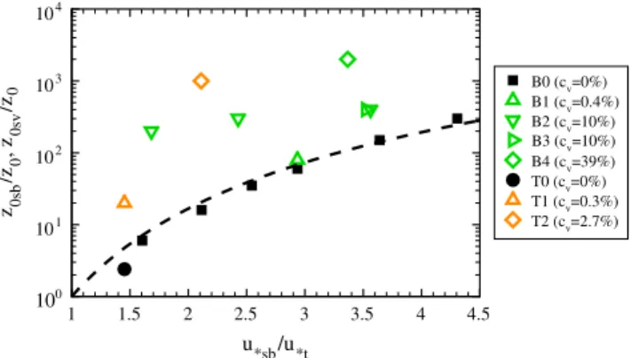
u_*sb/u_*t z0sb /z0 , z 0sv /z0 1 1.5 2 2.5 3 3.5 4 4.5 100 101 102 103 104 B0 (cv=0%) B1 (cv=0.4%) B2 (cv=10%) B3 (cv=10%) B4 (cv=39%) T0 (cv=0%) T1 (cv=0.3%) T2 (cv=2.7%)

Figure 6. Saltation roughness lengths over bare (z0sb) and vegetated (z0sv) surfaces as a function of the saltation friction velocity over

an equivalent bare sandu∗sb, deduced from all simulated cases. Roughness lengths are normalized by the ground roughness length

(z0), andu∗sbis normalized by the threshold friction velocityu∗t. The dashed black line fits dots of the bare sand case B0 (z0sb∕z0 =

(

Au2 ∗sb∕2g

)1−r

zr−1

0 withr = u∗t∕u∗sbandA = 0.21).

velocity above the vegetation and the roughness length of the vegetated surface should therefore weakly

change with saltation, and the roughness length should depend lightly on the wind conditions (i.e., u∗sbv).

Figure 6 presents the saltation roughness lengths (zosbfor bare sand and zosvfor vegetated surface),

nor-malized by the ground surface roughness length z0, as a function of u∗sbnormalized by its threshold value

u∗t. Despite the difference of mesh resolution and surface roughness length between bare sand cases B0

and T0, z0sb∕z0obtained in case T0 is in close agreement with, although slightly lower than, the relationship

between z0sb∕z0and u∗sb∕u∗tobtained in Du2013 for bare sand (equation (7)). As expected, zosvincreases with

vegetation cover and is higher for tree than for shrub cases for similar vegetation cover. For the same

veg-etation configuration (B3), zosincreases only slightly with increasing wind condition, confirming that the

momentum extracted by particles is negligible compared to that extracted by vegetation.

3.2. Sediment Transport

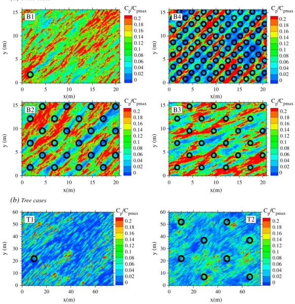
Figures 7a and 7b present an instantaneous view of the vertically integrated particle concentration field Cp

(number of particles per m2_{) normalized by its maximum value Cpmax, in the horizontal section x-y, for shrub}

(B1 to B4) and tree (T1 and T2) cases, respectively. Elongated patterns of high sand concentration in the mean wind direction, known as aeolian streamers [Baas and Sherman, 2005; Du2013], are present in shrub and tree cases, surrounded by regions with low concentration. Streamers present in tree cases have sim-ilar sizes as in shrub cases with low vegetation cover. However, for the densest shrub case (B4), streamer width appears larger and scales with the interrow width. Calling these latter sand structures “streamers” may be inaccurate as they remain channelized within the interrow region without meandering much. Since aeolian streamers are a visual footprint of past turbulent eddies propagating in the surface boundary layer [Du2013], flow structures of the size of shrub or interrow width are certainly driving saltating particles in the interrow region of case B4. In case T2, streamers do not appear as well aligned with the mean wind direc-tion as in T1 and shrub cases. This may be related to the presence of larger flow structures, scaling with individual trees and skirting around trees. In shrub cases, although intermittent high concentration clouds propagate from the interrow to the row regions, the sand concentration appears lower in the row regions because of the lower wind velocity (Figure 3) and the trapping of sand particles by shrubs. This distinction

between row and interrow regions is less visible for wind oriented at 22.5◦_{(B3) than at 45}◦_{(B2) because the}

distance between successive shrubs, L∕h, is larger in B3 (Table 1), allowing the flow to recover between suc-cessive shrubs. In tree cases, the row and interrow regions are imperceptible from the instantaneous sand concentration field as the wind reduction near the surface is spread over a larger area than in shrub cases. Figures 8a and 8b show for shrub and tree cases, respectively, the vertical profiles of the mean horizontal

mass flux⟨G⟩txy(g cm−2_s−1_{) normalized by the total saltation flux}⟨G

tot⟩txy(g cm

−1_s−1_{) and by the saltation}

layer height zm(see the next paragraph for a definition). For bare sand cases (B0 and T0),⟨G⟩txydecreases

exponentially with height as previously observed experimentally [Nalpanis et al., 1993; Greeley et al., 1996;

Rasmussen and Sorensen, 2008] and numerically [Kok and Renno, 2009; Du2013]. With vegetation,⟨G⟩txy

decreases exponentially only near the surface. In the upper saltation layer and above, this decrease is much lower as the particle concentration at this level is larger than in bare sand cases. This feature is enhanced

(a)

Shrub cases 15 15 10 5 0 y (m) 15 10 5 0 y (m) 60 50 40 30 20 10 0 y (m)

(b)

Tree cases 0 5 10 x(m) 15 20 0 5 10 x(m) 15 20 0 5 10 x(m) x(m) 15 20 0 5 10 x(m) 15 20 0 20 40 60 x(m) 0 20 40 60 0.2 C_p/C_pmax C_p/C_pmax 0.18 0.16 0.14 0.12 0.1 0.08 0.06 0.04 0.02 0 0.2 0.18 0.16 0.14 0.12 0.1 0.08 0.06 0.04 0.02 0.2 C_p/C_pmax C_p/C_pmax 0.18 0.16 0.14 0.12 0.1 0.08 0.06 0.04 0.02 0 0 0.2 0.18 0.16 0.14 0.12 0.1 0.08 0.06 0.04 0.02 0 C_p/C_pmax 0.2 0.18 0.16 0.14 0.12 0.1 0.08 0.06 0.04 0.02 0 C_p/C_pmax 0.2 0.18 0.16 0.14 0.12 0.1 0.08 0.06 0.04 0.02 0 60 50 40 30 20 10 0 y (m) 15 10 5 0 y (m) 15 10 5 0 y (m) B1 B4 B2 T1 B3 T2

Figure 7. Snapshot of horizontal cross section (x-y) of the vertically integrated sand concentrationC_pnormalized by its maximum value

Cpmaxfor (a) shrub and (b) tree cases. The case B2 corresponds to the simulation withu∗sb= 0.90m s −1

. The solid black circles represent the shrubs or the tree crowns.

〈G〉txyzm/〈Gtot〉txy

z(

m

)

10-3 ₁₀-2 ₁₀-1 ₁₀-0 ₁₀1

〈G〉txyzm/〈Gtot〉txy

10-3 ₁₀-2 ₁₀-1 ₁₀-0 ₁₀1 0.2 0.4 0.6 0.8 1 1.2 1.4 B0 B1 B2 B3 B4

(a)

Shrub cases Trees cases

z( m ) 0 0.5 1 1.5 T0T1 T2

(b)

Figure 8. Vertical profiles of the mean saltation flux⟨G⟩_txy(g cm−2_s−1_{) normalized by the total saltation flux}⟨G tot⟩txy(g cm

−1_s−1_{) and by}

the saltation layer heightzm, for (a) shrub and (b) tree cases. Cases B0 and B2 correspond to simulations withu∗sb= 0.54and 0.90 m s −1

, respectively. The dashed lines represent the shrub top (Figure 8a) and the lower tree crown level (Figure 8b).

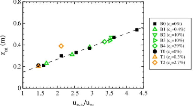
u_*sb/u_*t zm (m) 1 1.5 2 2.5 3 3.5 4 4.5 0 0.2 0.4 0.6 0.8

Figure 9. Saltation heightzmas a function of the saltation friction velocity over an equivalent bare sandu∗sb, normalized by the

threshold friction velocityu∗t, deduced from all simulated cases. The dashed black line fits dots of the bare sand case B0 (zm =

0.119u∗sb∕u∗t+ 0.029).

with vegetation cover and stronger in tree cases. The presence of larger flow structures scaling with plants is probably responsible for the upward transport of saltating particles. However, this upward transport

involves only a very small amount of particles and consequently a small portion of⟨Gtot⟩txy. In T0 and T1

cases, concentration profiles are almost identical.

The saltation layer height zmis deduced here from the mass flux profile because the momentum flux is

not constant above the saltation layer with the presence of vegetation. Hence, zmis deduced as the height

below which 99.5% of the total mass flux⟨Gtot⟩txyoccurs. Figure 9 presents for all cases, zmas a function of

u∗sb∕u∗t. As observed in Du2013, zmincreases linearly with u∗sb∕u∗tfor bare sand. More surprisingly, zm

val-ues do not depart much from a linear relationship in the presence of vegetation; zmis only slightly larger in

case T2. Although vertical saltation flux profiles of vegetated cases have different shapes than those over bare sands, these differences concern only a small number of particles. Consequently, the saltation layer height appears (1) weakly impacted by the presence of shrubs whatever their distribution, at least for the characteristics studied here, and (2) slightly larger in presence of trees for the densest configuration case.

3.3. Sand Erosion Patterns

The spatial distribution of the time average budget of sand erosion⟨Es⟩t, normalized by its maximum value,

is presented in Figures 10a and 10b, in a x-y plane, for shrub (B1 to B4) and tree (T1 and T2) cases.⟨Es⟩t

is the difference between the number of particles emitted per square meter and the number of particles

deposited on sand bed and on vegetation. Hence, negative values of⟨Es⟩tcorrespond to sand accumulation

and positive values to erosion. Although wind conditions differ between cases, the comparison of the

mag-nitude of accumulative and erosive regions is possible since⟨Es⟩tis normalized and since the sand erosion

reduction rate due to vegetation is weakly sensitive to wind condition (see section 4.2).

In shrub cases, distinct erosion patterns related to the vegetation distribution are visible. They correspond (1) to accumulation on the shrubs themselves because of sand trapping, (2) to sand accumulation on the lee of shrubs where the wind velocity is reduced as a consequence of vegetation wake effect (section 3.1), and (3) to erosion in the interrow region where the wind velocity is higher. The accumulation on shrubs rel-ative to the maximum erosion is higher in case B1 and lower in case B4. For the two cases with the same plant configuration (B2 and B3), the relative accumulation on shrubs is the largest in B3 where the distance between successive shrubs in the mean wind direction, L∕h, is the longest. This means that the relative deposition on shrubs decreases with L∕h. The amplitudes of sand accumulation and (sand erosion) on the lee of shrubs (in the interrow), relative to the maximum erosion, do not vary much. Accumulative regions overlap downwind of shrubs in cases B2 and B3 and appear longer in the lower vegetation cover case B1 than in B3. The relative sand erosion is slightly larger on shrub lateral sides of case B4.

In tree cases, erosion is observed on the lateral side of the trunks and upwind where the wind velocity is higher because of the flow skirting around the trees. Sand accumulates on the lee of trees over a region scaling with the tree size. Unlike in shrub cases, (1) particle are not trapped by trees as the saltation layer is located below the tree crowns and (2) no erosion is observed in the interrow region. The spatial variability of erosion is not as marked in tree cases as in shrub cases. Our explanation is that shrubs have a local impact by trapping particles and reducing locally the wind velocity while trees have a larger scale of influence by reducing the wind velocity in the lower atmospheric surface layer.

15 10 5 0 y (m) 15 10 5 0 y (m)

(a)

Shrub cases

0 5 10 15 20 x(m) 0 5 10 15 20 x(m) 0 5 10 15 20 x(m) 0 5 10 15 20 x(m) max 〈Es〉t/〈Es〉t 0.5 0 -0.5 -1 -1.5 -2 -2.5 -3 max 〈Es〉t/〈Es〉t 0.5 0 -0.5 -1 -1.5 -2 -2.5 -3 B1

(b)

Tress cases 50 40 30 20 10 0 y (m) 0 20 40 60 x(m) 0 20 40 60 x(m) max 〈Es〉t/〈Es〉t 0.5 0 -0.5 -1 -1.5 -2 -2.5 -3 max 〈Es〉t/〈Es〉t 0.5 0 -0.5 -1 -1.5 -2 -2.5 -3 0.5 0 -0.5 -1 -1.5 -2 -2.5 -3 max 〈Es〉t/〈Es〉t 0.5 0 -0.5 -1 -1.5 -2 -2.5 -3 max 〈Es〉t/〈Es〉t 50 60 40 30 20 10 0 y (m) 15 10 5 0 y (m) 15 10 5 0 y (m) B4 B3 B2 T1 T2

Figure 10. Spatial distribution of the time average budget of sand erosion⟨Es⟩tin ax-yplane normalized by its maximum value⟨Es⟩

max

t , for (a) shrub and (b) tree cases. Negative

values of⟨Es⟩tcorrespond to sand accumulation and positive values to sand erosion. The case B2 corresponds to the simulation withu∗sb = 0.90m s −1

. The dashed black circles represent the shrubs or the tree crowns.

Finally, we should remember that the patterns observed in Figure 10 applied to cases where the sand bed remains flat as assumed by constraint in these simulations. In the presence of vegetation, as erosion pro-ceeds, the bed surface should deform and therefore modify the near-surface wind flow. We will see in section 4.1 that the observed patterns from our simulations are consistent with previous wind-tunnel and field observations.

3.4. Saltation Flux

Since vegetation is commonly used to reduce sand erosion, one important outcome of our simulations is the estimation of the erosion reduction following vegetation characteristics. Figure 11 presents the

total saltation flux⟨Gtot⟩txysimulated in all cases as a function of u∗sb∕u∗t. Additionally, Table 1 presents

the values of the sand erosion reduction rate rerod(equation (9)) due to the presence of vegetation for all

u_*sb/u_*t 〈Gtot 〉txy (gcm -1s -1) 1 2 3 4 101 100 10-1 10-2 10-3

Figure 11. Total saltation flux⟨G_tot⟩_txyas a function of the saltation friction velocity over an equivalent bare sandu∗sbnormalized by the

threshold friction velocityu∗t, deduced from all simulated cases. The dashed black line fits dots of the bare sand case B0 (⟨Gtot⟩txy =

c√⟨d_p⟩∕D𝜌u3 ∗sb

(

1 − u∗t∕u∗sb

)

∕gwithD = 250_𝜇m andc = 1_.8for⟨G_tot⟩_txyin kilogram per meter per second).

As for the saltation roughness length,⟨Gtot⟩txyof case T0 is in close agreement with the relationship obtained

by Du2013 between⟨Gtot⟩txyand u∗sb∕u∗tfor bare sand. Dots related to vegetated cases are located below

this curve meaning that the presence of vegetation reduces sand erosion. For some specific configurations with sparse vegetation, Musick et al. [1996] and Burri et al. [2011] observed that the presence of vegetation elements increases sand erosion. They explained this feature by the formation of high wind speed regions, as observed in our simulation, that increase erosion without being balanced by a decrease of erosion behind

plants. This enhancement of erosion was not observed here. In case B2,⟨Gtot⟩txyappears to increase with

u∗sb∕u∗tas observed over bare sand but with a lower magnitude, corresponding to a sand erosion

reduc-tion of about 52%. This value slightly changes with wind condireduc-tion but without showing a clear tendency (Table 1). The erosion reduction increases with vegetation cover. For the same vegetation cover, the

mag-nitude of reroddiffers between shrubs and trees. A tree cover of 0.3% reduces erosion by 77%, while for the

same cover of shrubs (0.4%) the erosion reduction is only 8%. To reach a reduction of 77%, the shrub cover has to be between 10% and 39%. Finally, for the same shrub arrangement and cover, the erosion reduc-tion is on average 52% in case B2 and 72% in case B3, meaning that variareduc-tions in wind direcreduc-tion can impact significantly the sand erosion.

4. Discussion

In the previous section, we identified flow and sand erosion patterns related to vegetation characteristics and quantified the saltation flux reduction induced by the presence of the vegetation. In this section, we dis-cuss these findings by comparing them to observations reported in the literature and with simple predictive models of erosion reduction associated with vegetation characteristics.

4.1. Wind Flow and Sand Erosion Patterns

The flow regimes (isolated-roughness, wake interference and skimming flows) of each of the vegetation configurations have been identified in section 3.1 following the degree of interaction between wake zones developing behind vegetation elements. Lee and Soliman [1977] established a correspondence between these flow regimes and the concentration of surface roughness elements. This concentration is defined by the distance between successive plants in the mean wind direction L∕h, the vegetation cover cv, and the

roughness density𝜆 (the total frontal area of all plants divided by the total area) (Table 1). The criteria of Lee

and Soliman [1977], based on these vegetation characteristics, lead to the same flow regimes as the ones

deduced from our model, except for cases B2 and T2 that would be classified as isolated flow instead of wake interference flow.

The sand erosion patterns observed in all vegetated cases are related to wind field patterns and con-sequently to the flow regimes. This is consistent with the wind-tunnel observations of Sutton and

McKenna-Neuman [2008a, 2008b] who related the spatial variations of surface shear stress and turbulent

fluctuations to sediment entrainment near isolated, solid roughness elements. Sand accumulation regions behind vegetation elements appear correlated with the wake zones identified in section 3.1. This means that vegetation protects the surface on its lee side from saltation impacts and consequently from particle ejections. As a consequence, flow regimes can be identified from the degree of interaction between sand

C_v (%) 〈Gtot 〉txy /〈 Gtotb 〉txy 10-1 ₁₀0 ₁₀1 ₁₀2 10-3 10-2 10-1 100

Figure 12. Comparison between the present model (dots) and Lancaster and Baas’s [1998] predictive equation (dashed line) of the

total saltation flux⟨Gtot⟩txynormalized by its equivalent value over a bare sand⟨Gtotb⟩txyas a function of the vegetation covercv, for all

vegetated cases.

accumulation regions developing behind plants. This was done by Burri et al. [2011] from their wind-tunnel experiment.

In shrub cases, sand accumulation in the lee of plants as well as the degree of overlapping between the accumulations following the vegetation distribution, match very well with the patterns observed by

Burri et al. [2011] on a regular arrangement of small plants and with the formation of sand tails observed

by Sutton and McKenna-Neuman [2008b] in the lee of solid elements. However, contrary to Sutton and

McKenna-Neuman [2008b], we do not observe enhanced erosion in the far wake of shrubs. The role of small

vegetation in initiating accumulation regions and in initiating the formation of aeolian dunes is well known in semiarid and coastal environments. For example, Nebkha dunes are known as small ovoid dunes develop-ing behind small shrubs, resultdevelop-ing from sand accumulation on the shrub itself and on its lee side [e.g., Danin, 1996; Nield and Baas, 2008].

In tree cases, higher sand erosion around tree trunks (section 3.3) was observed by Leenders et al. [2007] in the Sahelian zone of Burkina Faso and on the lateral side of solid roughness elements by Sutton and

McKenna-Neuman [2008b] and McKenna-Neuman et al. [2013]. This is explained by the faster wind

veloc-ity around the trunk. A visualization of the spatial distribution of the saltation flux (not shown) exhibits the same patterns as those observed from the erosion budget, with a spatial variability of about 50% of the mean saltation flux. Saltation flux measurements performed by Labiadh et al. [2013] on a Tunisian orchard similar to case T2 did not identify a spatial variability of the flux between olive trees larger than the precision of the measurements. They obtained a spatial variability of about 17% of the mean flux. This value could be explained by the high variability of the wind direction during Labiadh et al.’s field erosion event,

con-tributing to smoother sand erosion patterns. Their standard deviation of wind direction was 95◦while in our

simulation the mean wind condition was constant, leading to a standard deviation of about 10◦.

In conclusion, the sand erosion patterns simulated in shrub and tree cases are qualitatively consistent with previous wind-tunnel and field observations. The regularity of these patterns may be smeared in reality as a consequence of large scale wind direction fluctuations during erosion events. Although our model neglects the deformation of the sand bed during an erosion event, it identifies the possible location of dune for-mation from erosion patterns. Specific models simulating the dynamics of dune forfor-mation in the presence of vegetation have been developed based on cellular automation algorithm [Nield and Baas, 2008]. While our model focuses on sand transport for individual erosion events, models of dune formation focus on the long-term sand surface dynamic by simplifying the sand transport. Our approach cannot simulate dune formation because of computational limitations, but it could improve the sand transport component in existing dune models.

4.2. Saltation Flux Reduction

As stated in section 1, Lancaster and Baas [1998] proposed a relationship between sand erosion reduc-tion and vegetareduc-tion cover. The equareduc-tion was deduced from measurements conducted at Owens Lake in

California with a cover of salt grass of about 0.10 m height. Figure 12 presents the total saltation flux⟨Gtot⟩txy

normalized by its equivalent value over bare sand⟨Gtotb⟩txyas a function of the vegetation cover cv. On the

same figure is shown the relationship proposed by Lancaster and Baas [1998] (dashed line).

For shrub cases, our model predicts less erosion reduction than the relationship of Lancaster and Baas [1998]. Furthermore, our model is sensitive to the wind direction relative to the plant distribution. For the

same vegetated surface (cases B2 and B3), the erosion reduction predicted by our model increases from

52% to 72% for a wind direction changing from 45◦_{to 22.5}◦_{. An additional simulation with a mean wind}

direction of 0◦_{showed an erosion reduction of 100%, as the saltation process ceased few minutes after}

its initiation (result not shown). The lower values of erosion reduction obtained from our model could be explained by the regular arrangement of shrubs relative to the main wind directions in cases B1, B2, and B4. In case B3, where the wind direction is not as well aligned with plant distribution, the erosion reduction is larger. This is consistent with field experiments where the presence of “streets” of bare soil was observed to increase the overall soil erosion in the mesquite landscape of the Chihuahuan desert [King et al., 2006;

Bowker et al., 2007]. On the other hand, for a similar shrub distribution as in the present study but with

dif-ferent shrub characteristics and spacing, Burri et al. [2011] obtained, from their wind-tunnel experiment, a sand erosion reduction in good agreement with Lancaster and Baas’s [1998] model. This could be related

(1) to the 0◦_{wind direction relative to their plant distribution that gave us an erosion reduction of 100%,}

(2) to their higher plant roughness density𝜆, or (3) to their bigger saltating particles (around 600 𝜇 m). In

tree cases the erosion reduction predicted by our model is higher than that predicted by Lancaster and

Baas’s [1998] equation. Since their relationship was obtained from small plants, it may not be applicable to

larger vegetation such as trees. Finally, vegetation cover may not be the best variable to characterize the impact of vegetation on sand erosion. The frontal area density may be more appropriate as it measures the momentum absorbed by the vegetation [Raupach et al., 1993]. However, sand erosion reduction as a func-tion of the frontal area density did not show a combined relafunc-tionship between shrub and tree cases (figure not shown). It is unclear how the roughness elements should be characterized to obtain, for any vegeta-tion morphology and distribuvegeta-tion, a unique relavegeta-tionship between the sand erosion reducvegeta-tion rate and a vegetation characteristic.

To confirm the sensitivity of erosion reduction to wind direction, and to verify that the low erosion reduc-tion obtained from our model in shrub cases is related to our specific distribureduc-tion of plants, we compare here our predictions in shrub cases B2, B3, and B4 with the ones deduced from the approach of Okin [2008] based on shear stress partitioning. Following his approach, we divided the sand bed of shrub cases into two regions: (1) the interrow region where the impact of shrubs on wind flow and saltation is neglected and the erosion is assumed equivalent to that over bare sand and (2) the row region where the ratio between

the local saltation friction velocity (uloc

∗sb) and the equivalent one in the absence of plants (u∗sb) is assumed to

increase exponentially downwind from the shrubs according to the measurements of Bradley and Mulhearn [1983]. The local saltation flux is then deduced from the parameterization of Shao et al. [1993] depending on uloc

∗sb∕u∗sb. In Table 1, the values of the erosion reduction r

∗

erodobtained from this approach are compared

with the values reroddeduced from our model. The approach of Okin [2008] exhibits the same trend as our

model following vegetation cover and wind direction. The magnitude of r∗

erodis similar to rerodin case B4 and

lower in other cases, with a difference going up to 20% in case B2 with u∗sb = 0.62 m s

−1_{. Predictions from}

Okin’s approach appear lower than those from our model, which are lower than Lancaster and Baas’

predic-tions. The fact that our model is not accounting for surface deformation as the erosion proceeds could be one of the reasons for such differences. Overall, this intercomparison confirms (1) that the vegetation dis-tribution following the mean wind direction has a significant impact on sand erosion reduction and (2) the magnitude of sand erosion reduction is significantly different from one approach to another although our approach and that of Okin [2008] exhibit the same sensitivity to shrub distribution.

4.3. Shrub Versus Tree

Trees appear to be more efficient to reduce sand erosion than shrubs. Although shrubs trap saltating parti-cles, the better efficiency of trees to reduce erosion is explained by the large-scale wind reduction induced by trees compared to the local sheltering effect of shrubs. This difference has been identified by Leenders

et al. [2007] from their field experiment although they were not able to conclude on the better efficiency

between trees and shrubs. They recommended using both types of vegetation to limit erosion.

From our simulations, shrubs appear subject to immersion while trees are subject to uprooting. Indeed, unlike shrubs, trees are not capable of trapping saltating particles as the height of their crowns starts well above the saltation layer. The factors responsible for sand erosion or accumulation following plant type have to be accounted for in orchard and crop management practices. For example, the alignment of the plants relative to the direction of the strongest winds and their distance relative to plant height could be considered in young crops in order to limit erosion in the interrow or to limit plant immersion.