Determination of the bulk melting temperature of
nickel using Monte Carlo simulations: Inaccuracy of
extrapolation from cluster melting temperatures
The MIT Faculty has made this article openly available.
Please share
how this access benefits you. Your story matters.
Citation
Los, J. H., and R. J. M. Pellenq. “Determination of the bulk melting
temperature of nickel using Monte Carlo simulations: Inaccuracy of
extrapolation from cluster melting temperatures.” Physical Review
B 81.6 (2010): 064112. © 2010 The American Physical Society.
As Published
http://dx.doi.org/10.1103/PhysRevB.81.064112
Publisher
American Physical Society
Version
Final published version
Citable link
http://hdl.handle.net/1721.1/57442
Terms of Use
Article is made available in accordance with the publisher's
policy and may be subject to US copyright law. Please refer to the
publisher's site for terms of use.
Determination of the bulk melting temperature of nickel using Monte Carlo simulations:
Inaccuracy of extrapolation from cluster melting temperatures
J. H. Los1and R. J. M. Pellenq1,2
1Département Théorie et Simulation Numérique, Centre Interdisciplinaire des Nanosciences de Marseille (CINaM), CNRS-UPR 3118, Campus de Luminy, 13288 Marseille, France
2Department of Civil and Environmental Engineering, MIT, 77 Massachusetts Avenue, Cambridge, Massachusetts 02139, USA 共Received 14 October 2009; revised manuscript received 20 January 2010; published 24 February 2010兲
We have determined the bulk melting temperature Tmof nickel according to a recent interatomic interaction model via Monte Carlo simulation by two methods: extrapolation from cluster melting temperatures based on the Pavlov model共a variant of the Gibbs-Thompson model兲 and by calculation of the liquid and solid Gibbs free energies via thermodynamic integration. The result of the latter, which is the most reliable method, gives Tm= 2010⫾35 K, to be compared to the experimental value of 1726 K. The cluster extrapolation method, however, gives a 325° higher value of Tm= 2335 K. This remarkable result is shown to be due to a barrier for melting, which is associated with a nonwetting behavior.
DOI:10.1103/PhysRevB.81.064112 PACS number共s兲: 64.75.⫺g, 64.70.D⫺, 82.60.Qr
I. INTRODUCTION
共Semi-兲empirical interatomic interaction models for real-istic atomreal-istic simulations of reactive processes including phase transitions have become quite popular due to their su-perior efficiency in comparison to methods based on ab initio theory and their improved accuracy during the last decades. Embedded atom methods,1–4 Stillinger and Weber type of
potentials,5–7bond order potentials,8–15and tight-binding
ori-ented potentials16–19 are examples of models that made a
significant evolution regarding their functional form and ac-curacy and have been parameterized for a variety of elements and mixtures. Of course, such potentials have to be thor-oughly tested and compared to experimental and ab initio data in order to assess their performance, their weak and strong points, and their reliability in various circumstances to which they were not fitted.
An important property that one typically would like to know, and that is commonly not included in the fitting pro-cess, is the bulk melting temperature Tmaccording to such a
model. In the present work, we have determined the melting temperature of the pure nickel component of a recent inter-esting semiempirical model19 for binary systems of carbon
共C兲 and nickel 共Ni兲, which is based on an efficient tight-binding共TB兲 scheme combined with the recursion method.20
A technologically quite relevant application possibility of this model is the study of the catalytic role of Ni in single wall carbon nanotube growth by atomistic simulation.21–23In
this growth process the Ni droplet is sticking to the open end of the growing tube and the carbon atoms are supplied from a共hydro兲carbon vapor phase via the Ni droplet to the tube. Knowledge of the bulk melting temperatures of the Ni com-ponent, which is an essential reference for the size dependent melting temperature of clusters, is of crucial importance for simulations of this process. Besides, it is an important test for the potential.
Accurate determination of Tmis not a trivial task due to
the large hysteresis that typically occurs during melting and recrystallizing of a system, especially for the bulk phase. One cannot simply heat up a crystalline bulk phase in a
simulation box with periodic boundary conditions and then say that Tm is equal to the temperature where the energy
makes a jump and/or disorder/diffusion is observed. This can lead to quite large errors as is indeed indicated by the fact that, typically, recrystallization by cooling the liquid phase occurs at a much lower temperature. This problem has been recognized and several methods have been proposed to avoid or reduce it. One possibility is to determine Tmby
extrapo-lation of the melting temperatures of clusters of increasing size on the basis of simple models, including Gibbs-Thompson-like models24,25 and models which include
sur-face melting.26 For clusters, hysteresis is expected to be
共much兲 smaller. However, as we will show, it can still be significant, up to an extent that it hinders an accurate deter-mination of Tm. A second method is to construct a simulation
box containing the solid and the liquid phase in contact with each other and then run simulations at various temperatures around a presumed estimate of Tmin order to find that
tem-perature for which the phase boundary does not move.27,28
However, even in this case, for nonrough surfaces, the results can be obscured by the presence of hysteresis, this time due to a two-dimensional共2D兲 nucleation barrier required for the formation of steps/islands on the solid surface.29From lattice
Monte Carlo 共MC兲 simulation based on the Kossel model it is well known that this 2D nucleation barrier can give rise to a large dead zone with zero growth rate in the growth rate curve.30However, for rough surfaces this is not the case and
this method can give accurate results for Tm as has been
demonstrated.27 The third, probably the most rigorous
method to determine Tm is the thermodynamic integration
method31which allows for straightforward calculation of the
free energy as a function of temperature 共or pressure兲 for both phases. Two examples of the application of this method are given in Refs. 32and33. In the present paper, we have used the first and the last mentioned methods. This allowed us to assess the reliability of the cluster extrapolation method by comparing it to the more rigorous thermodynamic inte-gration method.
In Sec. II we will give the basic ingredients of the TB model used for the total-energy evaluation in our MC
simu-lations. In Sec. III we briefly describe the standard models explaining the size dependence of the melting temperature of clusters and apply it to our simulations of the melting of Ni clusters. SectionIVpresents the thermodynamic integration method and the Tm resulting from it. The “discrepancy” of
the latter result with that from cluster extrapolation is re-solved in Sec. V. Section VI contains a brief summary and perspectives.
II. MONTE CARLO SIMULATION MODEL
Our Monte Carlo simulation model is based on an effi-cient TB scheme19 in which the total energy is equal to the
sum of atomic energies Eiof all atoms i = 1 , . . . N,
E =
兺
i N Ei=兺
i N共Erep,i+ Ecoh,i兲. 共1兲
In this expression, the repulsive atomic energy Erep,iis given
by
Erep,i= F
冉
兺
jVR共rij兲
冊
共2兲where VRis a spherical symmetric pair potential with a finite
cutoff, preferentially between the first and second neighbor distances and F is a functional to optimize the transferability of the model for variable coordination environments. The cohesive atomic energy Ecoh,i in Eq.共1兲 is given by
Ecoh,i=
冕
⬁ EF 共E −⑀i兲ni共E兲dE =兺
冕
⬁ EF 共E −⑀i兲ni共E兲dE 共3兲 where ni共E兲 is the local density of states 共LDOS兲 projectedon the atomic orbital and ni共E兲=兺ni共E兲 is the total
LDOS for atom i and where⑀iis the average cohesive energy
per electron in a free atom. To prevent spurious charge trans-fer which in reality should play a minor role in C-Ni systems for which the potential has been designed,19 a “local Fermi
energy” is defined by the constraint Zi=兰⬁ EF
ni共E兲dE where Zi
is the number of valence electrons corresponding to the basis of orbitals of atom i. The pure Ni component, used here, is described within the 3d basis of orbitals and Zi= 8.
The intrinsic computational gain of the model is based on the fact that the projected local density of states is approxi-mated by a continued fraction expansion,
ni共E兲 = − 1 lim⑀→0 1 z − a1i− b1 i z − a2i− b2 i z − a3i− b3i/共z − ...兲 in which the aijand bij共j=1,2...兲 are directly related to the moments 具i兩Hm兩i典 共m=1,2,...兲 with H the TB Hamil-tonian, and in which all higher order continued fraction co-efficients aij and bij 共j=3,4...兲 are taken equal to a2i and b2i, respectively. In practice, this constant tail prolongation of the continued fraction expression implies that only the first four moments 共m=1,2,3,4兲 have to be computed, an
approach which involves the neighborhood up to the second-nearest-neighbor shell. Within this approximation, the inte-gration in Eq. 共3兲 can be performed analytically.34
On top of the intrinsic gain in computational efficiency of this approach共no matrix diagonalization required兲, we real-ized a very efficient MC implementation of the method35 by maximally employing the locality of the changes in the con-tributions to the moments after a MC atomic displacement and by replacing the numerical integration 关Eq. 共3兲兴 by a
numerically stable version of the analytical solution in Ref.
34. For pure Ni systems considered here this led to a 400共!兲 times faster code, making the here presented simulations fea-sible.
III. MELTING OF CLUSTERS A. Gibbs-Thompson and Pavlov
In this section we briefly present the theoretical basis of the traditional, thermodynamic models which are commonly used to explain the melting behavior of clusters. This gives us the opportunity to define the symbols for the relevant thermodynamic quantities, which are reused in subsequent sections. In these models, it is assumed that the cluster can effectively be described in a spherically symmetric geometry. The free energy of a solid共s兲 or liquid 共l兲 cluster contain-ing N particles, GP,cl共N兲, surrounded by a more fluid phase, i.e., a liquid or vapor/vacuum 共v兲 phase, of the same pure species can be written as
GP,cl共N兲 = NgP+␥PP⬘AP共N兲 共4兲
where gPis the bulk free energy per particle in phase P共s or
l兲, ␥PP⬘ is the free energy per unit area of the surface
be-tween phase P and P
⬘
and AP共N兲 is the surface area of thecluster in phase P which is a function of N. The condition for equilibrium, i.e.,GP,cl/N = gP⬘, leads共for a spherical
clus-ter兲 to N共gP⬘− gP兲 − 2 3␥PP⬘AP共N兲 = ⌬gPVP− 2 3␥PP⬘AP共N兲 = 0 共5兲 where⌬g=gP⬘− gP,Pis the共number兲 density and VPis the
volume of the cluster in phase P. The Gibbs free-energy difference between the bulk liquid and solid phase is equal to
⌬g = ⌬h − T⌬s ⯝ ⌬h
冉
1 − T Tm冊
共6兲 where Tm is the bulk melting temperature and where ⌬h
= hl− hs and ⌬s=sl− ss are, respectively, the bulk enthalpy
and entropy difference between the two phases. At Tm,⌬h is
the melting heat or latent heat and ⌬s=⌬h/Tm the melting
entropy. However, whereas normally hP and sP have a
sig-nificant dependence on temperature, the temperature depen-dencies of⌬h and ⌬s are usually weak and often neglected, which justifies the most right-hand side of Eq.共6兲. Since the
external pressure is zero in this work, which is representative for ambient conditions, enthalpy is equal to energy, i.e., hP
= uP and⌬h=⌬u. Therefore, from now on we will use
en-J. H. LOS AND R. en-J. M. PELLENQ PHYSICAL REVIEW B 81, 064112共2010兲
ergy u, with ⌬u being the bulk melting energy. Combining Eqs. 共5兲 and 共6兲 straightforwardly leads to the
Gibbs-Thompson equation Tmcl Tm = 1 − 2␥sl s⌬uRs 共7兲 where Tmclis the melting temperature of the cluster, and Rsis
the 共effective兲 radius of the solid cluster.
In our case of a free cluster the situation is different and we should consider the equilibrium between a solid cluster and a liquid cluster with the same number of atoms. Now the equilibrium condition is Gl,cl/N
⬘
兩N=Gs,cl/N⬘
兩N. UsingEq. 共4兲, and taking into account the density difference
be-tween liquid and solid phase, this can be worked out to
共gl− gs兲N + 2 3共␥lvAl−␥svAs兲 = ⌬gsVs,cl+ 2 3共q␥lv−␥sv兲As = 0. 共8兲
where we defined q⬅共s/l兲2/3. Then, by substitution of Eq.
共6兲 into Eq. 共8兲, we find the Pavlov equation,
Tmcl Tm = 1 − 2 s⌬uRs,cl 共␥sv− q␥lv兲 ⬅ 1 − 2⌬␥sl s⌬uRs,cl 共9兲 where we defined ⌬␥sl⬅␥sv− q␥lv. So essentially the
Pav-lov equation is equal to the Gibbs-Thompson equation but with a different interpretation of the surface term, i.e.,␥slis
replaced by⌬␥sl. Equation共9兲 predicts a linear dependence
of Tmclon the inverse cluster radius, 1/Rs, with Tmcl
extrapo-lating to Tmat 1/Rs= 0.
B. Results and Pavlov interpretation of cluster simulations
In Fig.1several heating energy curves at different “heat-ing rates” in terms of MC cycles per degree and a cool“heat-ing curve obtained from MC simulations of a free Ni cluster with 1289 atoms are presented. The initial cluster, shown in Fig.
2共a兲, has the Wulff shape, minimizing the surface energy at 0 K according to our interaction model and is a regular trun-cated octahedron. As we can see in Fig. 1 there is a large hysteresis of 470°. The fact that the energy after cooling does not reach the solid base line of the heating curve is due to the fact that the recrystallized system contains defects, as is dem-onstrated in Fig. 2共d兲. Due to the large hysteresis it can be argued that the cluster melting temperature Tmcl cannot be
unambiguously derived from Fig.1. For sure Tmcllies within
the range marked by the sharp jumps in the heating and cooling curves, but this would imply an inaccuracy of 470/2° 共!兲 in this case. However, it is a known fact that in nature one can hardly supercool a solid, but the undercooling of a liquid phase is quite common. This is due to the fact that there is a nucleation barrier for crystallization. For melting no barrier is expected, especially for a cluster, with a perma-nent availability of kink sites at the edges of the surface. Using this fact implies that Tmclshould be taken close to the
jump in the heating curve. Here we adopt a procedure that is used in calorimetric measurements and which is illustrated in Fig.1. In this method Tmclis determined by the intersection
of the line along the sharp jump in the heating curve and the solid base line.
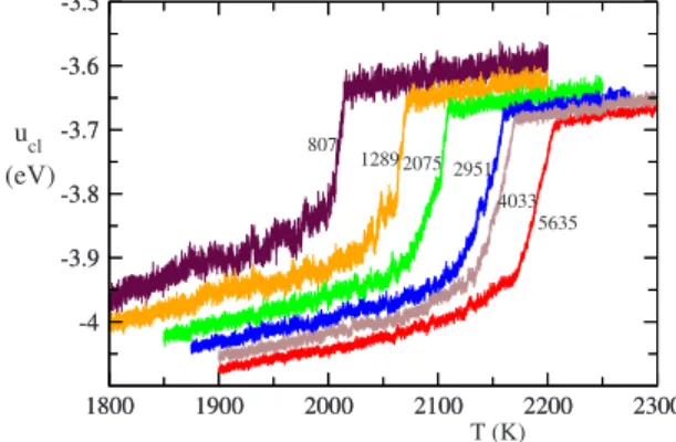
Determining Tmclin the described way for clusters with
the number of atoms ranging from N = 38 to N = 5635 共see Fig. 3兲, and plotting Tmcl against 1/Rs leads to Fig. 4. We
1400 1600 1800 2000 2200 -4 -3.9 -3.8 -3.7 -3.6 -3.5 -4 -3.9 -3.8 -3.7 -3.6 -3.5 T (K) heating cooling 470 degrees ! Tmcl Tc
solidbase line u (eV)
N=1289 atoms
60 30
15
FIG. 1.共Color online兲 Melting energy curves for “heating rates” of 15, 30, and 60 MC cycles per degree, as indicated in the graph 共one MC cycle is N MC atomic displacement trials兲, and a cooling energy curve for a “cooling rate” of 60 MC cycles per degree for a Ni cluster of 1289 atoms. Following the procedure in the experi-mental differential scanning calorimetry technique, the cluster melt-ing temperature Tmcl is determined by the intersection of the solid
phase base line 共lower dashed line兲 and the vertical dashed line located at the jump in the heating curve. The energy u is in eV per particle.
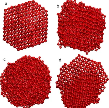
FIG. 2. 共Color online兲 共a兲 Initial Wulff-shaped configuration, snapshots共b兲 during heating just before melting and 共c兲 after melt-ing, and共d兲 final recrystallized configuration after cooling. These configurations belong to the system and simulations with the slow “heating and cooling rates” of Fig.1. Note that the共d兲 recrystallized state is not monocrystalline in this case.
have taken on purpose a systematic sequence of Wulff clus-ters so that the solid-vapor interfacial energy is similar for each cluster and a smooth dependence of the melting tem-perature on the 共inverse兲 cluster size can be expected facili-tating the extrapolation to the bulk crystal. The best straight-line fit of the cluster melting temperatures of the 6 largest clusters extrapolates, according to the Pavlov expression, to a bulk melting temperature of Tm= 2335 K, well above the
experimental value Tm,exp= 1726 K.
IV. THERMODYNAMIC INTEGRATION A. Thermodynamic integration method
The method of thermodynamic integration to determine the bulk melting temperature is based on the calculation of the Gibbs free energies as a function of temperature共or pres-sure兲 for both the liquid and the solid phases. Then, the melt-ing temperature at a given pressure共or the equilibrium pres-sure at a given temperature兲 is given by the intersection of
the two curves. In our case we will determine Tmat a
pres-sure P0= 0.
For both liquid and solid phases the calculation based on MC simulation consists of four steps. In step 1 the equilib-rium volume, Veq, at P0and a temperature T0close to a first estimate of Tmis determined by means of共NPT兲 MC
simu-lation. Next, in step 2, the so-called-integration 共see below兲 is performed to calculate the Helmholtz free energy FP in
phase P = l , s from the known Helmholtz free energy of a reference system, FP,ref, by means of共NVT兲 MC simulations at temperature T0 and volume Veq. Subsequently, in step 3,
the Gibbs free energy at 共P0, T0兲 is evaluated by GP= FP
+ P0Veq. Finally, in step 4, the  integration 共see below兲 is
performed to compute GP共P0, T兲 as a function of T by means of共NPT兲 simulations at P= P0for a discrete grid ofvalues 共=共kBT兲−1兲.
In the integration, the energy of the system is given by UP共兲 = 共1 − 兲UP,ref+UP,TB 共10兲
where UP,ref is the energy of the reference system of known
free energy and UP,TB is the energy according to our TB
model. The Helmholtz free energy being equal to −−1ln Q共N,Veq, T0兲, with Q=dB
−3N兰drNexp共−
U共兲兲 the partition function at共N,Veq, T0兲 and dBthe de Broglie wave
length, it follows that dFP d = − 1  d dln Q =具UP,TB− UP,ref典 ⇒ FP= FP,ref+
冕
0 1 d具UP,TB− UP,ref典 共11兲 For the liquid phase the reference system is a Lennard-Jones共LJ兲 liquid described by so-called “cut and shifted” LJ potential, Ul,LJ=共r兲 −共rc兲 = 4⑀冉冉
r冊
12 −冉
r冊
6冊
−共rc兲 共12兲for r⬍rcand Ul,LJ= 0 for rⱖrc, where共r兲 is the standard
12-6 LJ potential and where rc= 4. The LJ parameters were
taken equal to ⑀= 0.21 eV and = 2.1 Å. These parameters were chosen such that 共i兲 LJ liquid is supercritical to avoid phase separation, and 共ii兲 the structure of the LJ liquid re-sembles that of the TB model by matching the positions of first peak in the radial distribution function, to optimize the numerical conditions of the calculation. The Helmholtz free energy Fl共, T兲 as a function of the density and T for this LJ
system has been accurately parameterized in Ref.36and we used this parametrization.
For the solid phase, the Einstein crystal was taken as ref-erence system, with the potential energy as a function of the atomic positions rigiven by
Us,Einst=
兺
i
共␣共ri− ri,ref兲2+ u0兲 共13兲 with␣a spring constant and u0an irrelevant shift and where
ri,ref are the fixed positions of the Einstein reference lattice,
which is a perfect fcc lattice in our case. The Einstein model
1800 1900 2000 2100 2200 2300 -4 -3.9 -3.8 -3.7 -3.6 -3.5 1800 1900 2000 2100 2200 2300 -4 -3.9 -3.8 -3.7 -3.6 -3.5 807 1289 2075 2951 4033 5635 ucl T (K) (eV)
FIG. 3. 共Color online兲 Melting energies curves for six Ni clus-ters. The cluster melting temperatures, Tmcl, which are used in Fig. 4are determined following the procedure illustrated in Fig.1.
0 0.05 0.1 0.15 0.2 1500 2000 2500 1/Rs(A-1) Tm(K) 38 201 405 2075 Tm=2335 K 5635 (Tm,exp=1726) Tc,0=2339 K 1/Rs(A-1) 0 0.05 0.1 1750 2000 2250 Tc(K) 5635 1289 201
FIG. 4. 共Color online兲 Cluster melting temperatures Tmcl
共sym-bols兲 as a function of the inverse cluster radius, 1/Rs. The dashed
straight line is a linear fit, which extrapolates to a bulk melting temperature of 2335 K. The symbols in the inset give the tempera-ture at which the barrier for melting vanishes, Tc共see Fig.1兲 versus
1/Rs. The dashed line in the inset is a straight-line best fit to the Tc’s of largest six clusters, whereas the full line is a best fit based on Eqs.共17兲 and 共18兲.
J. H. LOS AND R. J. M. PELLENQ PHYSICAL REVIEW B 81, 064112共2010兲
yields an analytical solution for the dimensionless Helmholtz free energy per particle,
Fs,Einst N =u0+ 3 ln共dB兲 − 3 2ln
冉
2 ␣冊
− 1 N冋
3 2ln冉
N ␣ 2冊
+ ln冉
V N冊
册
共14兲 where the fourth共last兲 term on the right-hand side represents the finite-size correction for keeping the center of mass fixed during the simulation, necessary to avoid divergence of the Einstein reference energy for→1. V is the volume of the simulation box containing N atoms. The Einstein potential parameters were taken equal to ␣= 12.8 eV/Å2, giving about the same mean-square displacement of the atoms as for the TB model, and u0= −5 eV, comparable to the TB model ground-state energy of −4.44 eV per atom.Since P0= 0 is our case, the Gibbs free energy at共P0, T0兲 is just GP共P0, T0兲=FP共P0, T0兲. Finally, using G共兲 = −−1ln Q共N, P
0, T兲 with Q共N, P0, T兲=dB
−3N兰dVdrNexp
共−共U+ P0V兲兲 the partition function at 共N, P0, T兲, GP共P0, T兲 at any T can be computed by integrating
dG d =具U + PV典 ⇒G共兲 =0G共0兲 +
冕
0  d⬘
具U + P0V典⬘ 共15兲 where具U+ P0V典⬘is determined in共NPT兲 MC simulation at P = P0.B. Bulk melting temperature from thermodynamic integration
Figure 5 shows the results for the simulations and the Gibbs free energies as a function of T resulting from the  integrations. To investigate size effects these calculations
were done for two systems of different sizes. The integra-tion was performed at different temperatures T0 for the two systems to check consistency. In all cases a cubic simulation box was used. The numbers of atoms in the two systems were N = 256 and N = 500, and the corresponding T0 was taken to be equal to 2300 and 2100 K, respectively. The first T0= 2300 K was based on our estimate from the cluster ex-trapolation method. To check for hysteresis, indicating un-desired phase changes, the simulations for the integration were first done for values from =0 to =1 in steps of d=0.1. After that, starting from the final configuration at =1, simulations were done for another set of values go-ing back from=0.95 to =0.05, again in steps of d=0.1, giving a total of 21 simulation points to perform the integra-tion in Eq. 共11兲 based on spline interpolations between
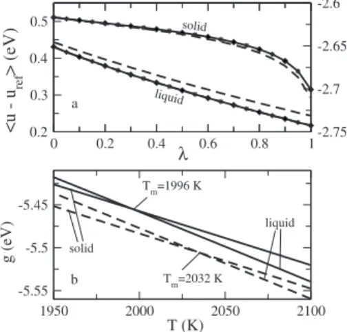
points. As we can see in Fig.5共a兲, no hysteresis occurs since all points are situated on a smooth curve, both for the solid and the liquid phases. Values of the various free-energy con-tributions are listed in TableIfor both systems. The intersec-tion points in Fig.5共b兲give bulk melting temperatures equal to Tm,256= 2032⫾45 K, and Tm,500= 1996⫾40 K for the
two systems. Although the results for the two systems are within the error margins, a difference of 36° is not very small. Although it can reasonably be expected that our result is converged, it might be interesting to perform a more de-tailed study of the size effects, which however is beyond the scope of the present paper. The experimental Tmbeing equal
to 1728 K, our result for Tm can be considered as a quite
reasonable performance of the TB interaction model and is considerably better than the prediction based on extrapola-tion in Sec. III B.
After thoroughly checking and verifying the thermody-namic integration calculations, also by performing them with independently developed software tools for computing the free energy of the LJ liquid according to Johnson and the Einstein crystal, we consider these results much more reli-able than those from cluster extrapolation as they are deter-mined from a rigorous method without suffering from the metastability phenomena associated with the large hysteresis as observed in the cluster simulations. Hence, we conclude that Tmis about 2010⫾35 K, which leaves us to explain the
“discrepancy” with the cluster extrapolation result.
V. ANALYSIS OF CLUSTER DATA BEYOND PAVLOV, CELESTINI MODEL
In the Celestini model the cluster is not necessarily com-pletely liquid or solid, like in the Pavlov model, but it may 0.2 0.3 0.4 0.5 a b 0 0.2 0.4 0.6 0.8 1-2.75 -2.7 -2.65 -2.6 λ < u-u ref > (eV) 1950 2000 2050 2100 -5.55 -5.5 -5.45 Tm=2032 K Tm=1996 K solid liquid solid liquid g (e V) T (K)
FIG. 5. 共a兲 Simulation results for the integrand 具u−uref典in the integration 关Eq. 共11兲兴 for the solid phase 共with labels on the left
vertical axis兲 and the liquid phase 共with labels on the right vertical axis兲, and 共b兲 the solid and liquid Gibbs free energies 共in eV per particle兲 as a function of T resulting from the integration 关Eq. 共15兲兴. The dashed and full lines are for the system with N=256 and
N = 500, respectively.
TABLE I. Values of the various free-energy contributions in the thermodynamic integration procedure where0=共kBT0兲−1, F
P,ref,0,
and FP,TB,0refer to the values at T0and I=兰10d具UP,TB− UP,ref典. Note that T0is different for the two system sizes共see text兲.
N = 256 N = 500
Liquid Solid Liquid Solid
0FP,ref,0/N −15.3197 −30.9277 −15.6898 −33.0325
0I/N −13.5784 2.2783 −14.9218 2.5276
also consist of a 共spherical兲 solid core surrounded by a 共spherical兲 liquid surface layer. It departs from the following expression for the Gibbs free energy of the cluster:
Gcl共Rsc兲 = glsVs−⌬gsVsc+␥slAsc+␥lvAcl
+⌬␥slvexp
冉
Rsc− Rs
冊
As 共16兲where␥slis the solid-liquid surface free energy and⌬␥slvis
the so-called spreading parameter defined as ⌬␥slv⬅␥sv
−␥lv−␥sl. Vcland Vsc are the spherical volumes of the total
cluster and the solid core with radii Rcland Rscand surface
areas Acland Asc, respectively, andis a length representing
the decay distance of the interaction between the sl and the lv surfaces. As and Vs are the surface area and volume of a
completely solid cluster as before, withsVs=lVl= N. It has
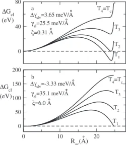
been shown that Eq. 共16兲 with positive ⌬␥slv can describe surface melting. This is illustrated in Fig. 6共a兲 where we plotted Gcl共Rsc兲−Gcl共0兲 against Rsc for a large Ni cluster
with 5635 atoms at different temperatures Ti共i=1, ...4兲,
us-ing values for␥sl andwhich are derived from a fit of the
model to the simulation data 共see below兲. For T=T1, Gcl共Rsc= Rs兲=Gcl共0兲; i.e., the completely liquid cluster and
the completely solid cluster are equally stable. However, Gcl
has a minimum at a solid core radius Rsc⬍Rs, which implies
surface melting. For the T = T2, the free energy of this coex-istence state with a solid core and a liquid layer becomes equal to that of the completely liquid cluster. For T2⬍T ⬍T4, the completely liquid cluster would be the most stable state but there is an energy barrier for melting. This barrier vanishes at T4, which we will call Tc. At Tc, dGcl/dRsc
= d2Gcl/d2Rsc= 0 and these conditions can be worked out to
Tc Tm = 1 − 2␥sl s⌬uRsc 共1 −/Rsc兲 共1 – 2/Rsc兲 共17兲 as has been presented by Celestini et al. Since we have two conditions, i.e., dGcl/dRsc= 0 and d2Gcl/d2Rsc= 0, a second
equation can be derived for Rsc, which for ⰆRsc can be
approximated by
Rsc⯝ Rs+ln
冉
2␥sl2
⌬␥Rs2
冊
. 共18兲
If we substitute Eq. 共18兲 into Eq. 共17兲, we obtain Tc as a
function of 1/Rs, allowing for a straightforward fit to obtain
values for Tm,␥sl,⌬␥, and. Since␥slis normally positive,
Eq. 共17兲 tells us that Tcshould be below Tmfor any cluster
size. Therefore, if we rely on the Tm= 2010 K from the
ther-modynamic integration method, Eq. 共17兲 can never explain
our results. From a best fit of Eq.共17兲, after substitution of
Eq. 共18兲, to the Tc’s of all clusters except the smallest with
N = 38 atoms, shown in the inset of Fig. 4, we find Tm
= 2339 K, ␥sl= 25.5 meV/Å, ⌬␥= 3.25 meV/Å, and
= 0.31 Å, which were used for Fig.6共a兲. So the predicted Tm
from this model is close to that predicted by the Pavlov model in this case. However, since the number of parameters is rather high with respect to the available simulation data, the accuracy of␥sland especially⌬␥, estimated on the basis
of just the fitting process, is not very high, with errors of about 20% and 40%, respectively. Instead, the error for Tmis
much smaller in the sense that the range of Tmvalues
allow-ing for a reasonable fit accordallow-ing to this model and positive ⌬␥is restricted to 2330⬍Tm⬍2350 K.
In the usually not considered case that⌬␥slv⬍0 the situ-ation becomes different. This is illustrated in Fig. 6共b兲. For the surface parameters indicated in the figure, at T1= 1982, below Tm, the free energy of a completely liquid cluster is
equal to that of a completely solid cluster. However, there is a large barrier for melting and there is no minimum at some Rsc⬍Rs, which means that surface melting is energetically
not favorable due to a large␥sland/or a small ␥sv−␥lv. For
the other temperatures, all well above Tm= 2010 K, the
com-pletely liquid cluster is more stable, but there is a significant barrier for melting. Finally, at T4= Tc= 2162 K, 150° 共!兲
above Tm, this barrier vanishes. Now the condition at Tc is
dGcl/dRsc兩Rcl=Rs which leads to Tc Tm = 1 − ⌬␥slv s⌬u − 2␥sl s⌬uRs . 共19兲
This equation predicts a linear dependence of Tc on 1/Rs,
similar to what the Pavlov equation does for Tmcl. However,
in the large cluster limit Tcdoes not converge to Tm, but to a
higher temperature Tm−⌬␥slvTm/共s⌬u兲. This behavior is
fully consistent with our simulations results for Tc versus
1/Rs, shown in the inset of Fig.4, where Tchas been
deter-mined as indicated in Fig.1. In fact, from the inset of Fig.4
and with taken equal to 6 Å, the surface parameters ␥sl
= 35.1 meV/Å2 and ⌬␥
slv= −3.33 meV/Å2 used in Fig.
6共b兲, are obtained by the slope and the intersection with the vertical axis at 1/Rs= 0, respectively, of a best linear fit
through the temperatures Tc. Thus, the Celestini model, but
0 40 80 a ∆γslv=3.65 meV/A γsl=25.5 meV/A ξ=0.31 A b ∆γslv=-3.33 meV/A γsl=35.1 meV/A ξ=6.0 A ∆Gcl T1 T2 T3 T4=Tc T4=Tc T3 T2 T1 (eV) ∆Gcl (eV) Rsc(A) 0 10 20 0 50 100 150 200
FIG. 6. The cluster Gibbs free-energy difference ⌬Gcl = Gcl共Rsc兲−Gcl共0兲 against the solid core Rscfor共a兲 positive and 共b兲
negative spreading parameter ⌬␥slv=␥sv−␥lv−␥sl. The tempera-tures in graph 共a兲 are T1= 2081, T2= 2100, T3= 2136, and T4= Tc
= 2172 K, whereas those in graph共b兲 are T1= 1982, T2= 2040, T3 = 2100, and T4= Tc= 2162 K.
J. H. LOS AND R. J. M. PELLENQ PHYSICAL REVIEW B 81, 064112共2010兲
with a negative⌬␥slv, can describe a cluster melting process without surface melting, i.e., a nonwetting behavior. In that case the melting can be retarded by a significant barrier, which for the larger clusters lead to melting temperatures well above Tm. In fact, in snapshot b of Fig. 2, taken at a
temperature just before complete melting, the nonwetting be-havior is confirmed by the fact that large parts of the surface are still ordered, and that some surface melting only takes place at the corners of the solid cluster, which can explain the change in the slope in the energy curves before melting. We also note that a decay length of 6 Å for the interaction between the sl and the lv surfaces seems much more realistic than the value = 0.31 Å that followed from the best fit of Eq. 共17兲 to the simulation data.
To some extent, one can argue that the observed retarda-tion of melting is a matter of time scale of the simularetarda-tion. However, we slowed down the “heating rate” until the melt-ing temperature did not change anymore共see Fig. 1兲. Thus,
in practice, this problem is difficult to control and under-mines the reliability of the determination of Tmby
extrapo-lation from the cluster melting temperatures. Note that this is also true for the case that ⌬␥slv⬎0 with surface melting.
Indeed, looking at Fig.6共a兲, the melting of the cluster could occur at any temperature between T2 and Tc. In addition,
from the cluster melting data alone, i.e., without knowing Tm
or having information about surface melting, it cannot even be decided whether⌬␥slv is positive or negative.
It is interesting to compare our values for␥sl with those
from the Turnbull expression37,38
␥sl= CTLs2/3 共20兲
where L⯝⌬u is the latent heat per atom and CT is the
so-called Turnbull coefficient, which was originally estimated to be equal to CT= 0.45 for metals. Recent efforts based on
atomistic simulation39–41have roughly confirmed the validity
of the Turnbull expression, but with somewhat larger values for CTbetween 0.47 and 0.6共Ref. 42兲 for an fcc crystal. In
our case this corresponds to 33.3⬍␥sl⬍42.6 meV/Å2, a
range which is consistent with the value based on Eq.共19兲
and larger than that from Eq.共17兲.
The nonwetting behavior we find is contrary to previous results for Ni cluster melting,43based on a bond order type of
potential.44,45 So the disagreement may come from the
dif-ference in the interaction potentials. For our TB model we can say that it reproduces reasonably well the surface ener-gies of several flat sv surfaces.19 On the other hand, the
disagreement may also be due to the fact that we started from Wulff clusters, minimizing␥sv and consequently⌬␥slv. It is
indeed more likely for a Wulff cluster to have a negative spreading parameter than for less stable clusters.
To conclude, we now give an extension of the Celestini model which includes the difference in density between liq-uid and solid phase. For a not too large density difference, the cluster surface Aclas a function of the solid core radius
Rscis very well approximated by
Acl共Rsc兲 = qAs+共1 − q兲
Rsc
Rs
Asc 共21兲
where q=共s/l兲2/3 as before. Equation 共21兲 yields Acl共Rsc
= Rs兲=As, Acl共Rsc= 0兲=qAs= Al, and Acl= As for any Rsc if
s=l, as it should be. Substitution of Eq.共21兲 into Eq. 共16兲
leads to Gcl共Rsc兲 = glsVs−⌬gsVsc+
冉
共1 − q兲 Rsc Rs ␥lv+␥sl冊
Asc + q␥lvAs+⌬␥slvexp冉
Rsc− Rs 冊
As 共22兲For Rsc= Rs and Rsc= 0 共with a vanishing exponential term
for Rsc= 0兲, Eq. 共22兲 is consistent with Eq. 共4兲. With Eq. 共22兲
and negative spreading parameter ⌬␥slv, the condition dGcl/dRsc兩Rcl=Rs= 0 at Tcnow leads to Tc Tm = 1 − ⌬␥slv s⌬u −2␥sl+ 3共1 − q兲␥lv s⌬uRs 共23兲
which gives back Eq.共19兲 for q= 1. According to Eq.共23兲,
the straight-line analysis shown in the inset of Fig. 4 still make sense, but the extraction of␥sl from the slope is much
more difficult since ␥lv and also q for a cluster are not 共accurately兲 known. However, since q⬎1 and ␥lv⬎0, the
induced correction for ␥sl is positive.
Finally, for the wetting case, i.e., for positive ⌬␥slv, the
expression for Tc/Tm including the density difference,
de-duced by imposing dGcl/dRsc= d2Gcl/d2Rsc= 0 with Gclfrom
Eq. 共22兲, becomes Tc Tm = 1 − 2␥sl s⌬uRsc 共Rsc−兲 共Rsc− 2兲 −3共1 − q兲␥lv s⌬uRs . 共24兲
In the limit of large clusters both correction terms at the right-hand side vanish, so that Tc→Tmin this limit. As in the
nonwetting case, the correction of␥sldue to the last term on
the right-hand side of Eq.共24兲 will be positive.
VI. SUMMARY, PERSPECTIVES
We have determined the bulk melting temperature Tmof
the pure Nickel component of a recent semiempirical inter-atomic interaction model,19 based on a TB framework, for
binary C-Ni systems via MC simulation. Rigorous calcula-tion of the Gibbs free energies for the liquid and solid phases by using the thermodynamic integration method leads to Tm= 2010⫾35 K, not too far from the experimental melting
temperature Tm,exp= 1726 K.
We also performed simulations of the melting of a se-quence of Wulff clusters, with sizes ranging from N = 38 to
N = 5635 atoms. Plotting the observed cluster melting tem-peratures against the inverse cluster radius gives approxi-mately a straight line, but extrapolation of this line according to the Pavlov equation suggests a Tmequal to 2335 K, 325°
higher than the Tm from thermodynamic integration. We
found an explanation for the observed “discrepancy” by ana-lyzing our cluster data in terms of the Celestini model. How-ever, contrary to the usual case, for which the Celestini model gives an appropriate correction to the Pavlov model due to the effect of surface melting, our data require a nega-tive value for the spreading parameter⌬␥=␥sv−␥lv−␥sl,
im-plying a nonwetting behavior, i.e., no surface melting occurs, or at least it does not occur at the usual relatively low tem-peratures as predicted when⌬␥ is positive. We have shown by Eq. 共19兲 关or Eq. 共23兲兴 that for negative ⌬␥ the cluster melting temperature against the inverse radius follows a straight line, which, however, does not extrapolate to Tmin
the large cluster limit but to a higher temperature. This can explain our observation of cluster melting temperatures lying above Tm for the large clusters due to a barrier for melting
which only vanishes at a Tc⬎Tm.
Usually, in literature, the Tm resulting from cluster
ex-trapolation is not compared with that from the more rigorous thermodynamic integration method, the latter method being more complicated and laborious. Here we have shown that a
straight line of the observed cluster melting temperature against the inverse cluster radius is no guarantee for a good approximation of Tmvia extrapolation.
Since our finding is remarkable, one should be careful with definitive conclusions. Theoretically it could be possible that the Johnson expression and/or parametrization36 for the LJ liquid is so inaccurate, contrary to what is claimed and what in commonly believed, that it can give rise to an error in Tmof more than 300 K. It would be very useful to have an
independent confirmation of our results, for example, by an alternative and accurate determination of the effective surface-free energies␥svand␥lv, which should be enough to
enable such confirmation. While it seems that ␥sl can be
determined rather accurately nowadays using recent simula-tion techniques,39–41,46,47 it is not so clear to which extent
these techniques and/or results can be used for or extrapo-lated to sv and especially lv surfaces. It would be very useful to find an answer to these questions and, if necessary, to develop additional techniques for the determination of ␥sv and␥lv.
ACKNOWLEDGMENT
We wish to thank PAN-H ANR共Mathysse兲 for support.
1M. W. Finnis and J. E. Sinclair, Philos. Mag. A 50, 45共1984兲. 2M. I. Baskes, Phys. Rev. Lett. 59, 2666共1987兲.
3M. I. Baskes, J. S. Nelson, and A. F. Wright, Phys. Rev. B 40, 6085共1989兲.
4J. Cai and J.-S. Wang, Phys. Rev. B 64, 035402共2001兲. 5F. H. Stillinger and T. A. Weber, Phys. Rev. B 31, 5262共1985兲. 6J. F. Justo, M. Z. Bazant, E. Kaxiras, V. V. Bulatov, and S. Yip,
Phys. Rev. B 58, 2539共1998兲.
7N. A. Marks, Phys. Rev. B 63, 035401共2000兲. 8J. Tersoff, Phys. Rev. Lett. 56, 632共1986兲. 9J. Tersoff, Phys. Rev. B 38, 9902共1988兲. 10D. W. Brenner, Phys. Rev. B 42, 9458共1990兲.
11D. W. Brenner, O. A. Shenderova, J. A. Harrison, S. J. Stuart, B. Ni, and S. B. Sinnott, J. Phys.: Condens. Matter 14, 783共2002兲. 12A. C. T. van Duin, S. Dasgupta, F. Lorant, and W. A. Goddard
III, J. Phys. Chem. A 105, 9396共2001兲.
13A. C. T. van Duin, A. Strachan, S. Stewman, Q. Zhang, X. Xu, and W. A. Goddard III, J. Phys. Chem. A 107, 3803共2003兲. 14J. H. Los and A. Fasolino, Phys. Rev. B 68, 024107共2003兲. 15J. H. Los, L. M. Ghiringhelli, E. J. Meijer, and A. Fasolino,
Phys. Rev. B 72, 214102共2005兲.
16D. G. Pettifor, Phys. Rev. Lett. 63, 2480共1989兲.
17D. G. Pettifor and I. I. Oleinik, Phys. Rev. B 59, 8487共1999兲. 18I. I. Oleinik and D. G. Pettifor, Phys. Rev. B 59, 8500共1999兲. 19H. Amara, J. M. Roussel, C. Bichara, J. P. Gaspard, and F.
Du-castelle, Phys. Rev. B 79, 014109共2009兲.
20R. Haydock, V. Heine, and M. J. Kelly, J. Phys. C 5, 2845 共1972兲.
21C. Journet, W. K. Maser, P. Bernier, A. Loiseau, M. Lamy de la Chapelle, S. Lefrant, P. Deniard, R. Lee, and J. E. Fischer,
Na-ture共London兲 388, 756 共1997兲.
22J. Gavillet, A. Loiseau, C. Journet, F. Willaime, F. Ducastelle, and J.-C. Charlier, Phys. Rev. Lett. 87, 275504共2001兲. 23J. Gavillet, J. Thibault, O. Stephan, H. Amara, A. Loiseau, C.
Bichara, J.-P. Gaspard, and F. Ducastelle, J. Nanosci. Nanotech-nol. 4, 346共2004兲.
24P. Buffat and J. P. Borel, Phys. Rev. A 13, 2287共1976兲. 25P. Pavlov, Z. Phys. Chem., Stoechiom. Verwandtschaftsl. 65, 1
共1909兲; 65, 545 共1909兲.
26F. Celestini, R. J.-M. Pellenq, P. Bordarier, and B. Rousseau, Z. Phys. D: At., Mol. Clusters 37, 49共1996兲.
27J. R. Morris and X. Song, J. Chem. Phys. 116, 9352共2002兲. 28For a review of the method, see F. D. Di Tolla, E. Tosatti, and F.
Ercolessi, in Monte Carlo and Molecular Dynamics of Con-densed Matter Systems, Conference Proceedings, edited by K. Binder and G. Ciccotti共SIF, Bologna, 1996兲, Vol. 49, Chap. 14, p. 346.
29W. K. Burton, N. Cabrera, and F. C. Frank, Philos. Trans. R. Soc. London, Ser. A 243, 299共1951兲.
30G. H. Gilmer and P. Bennema, J. Cryst. Growth 13-14, 148 共1972兲.
31A review of the method is given in: D. Frenkel and B. Smit, Understanding Molecular Simulation共Academic Press, San Di-ego, CA, 2002兲.
32E. J. Meijer and D. Frenkel, J. Chem. Phys. 94, 2269共1991兲. 33L. M. Ghiringhelli, J. H. Los, E. J. Meijer, A. Fasolino, and D.
Frenkel, Phys. Rev. Lett. 94, 145701共2005兲.
34G. Allan, M. C. Desjonqueres, and D. Spanjaard, Solid State Commun. 50, 401共1984兲.
35J. H. Los, C. Bichara, and R. J. M. Pellenq共unpublished兲.
J. H. LOS AND R. J. M. PELLENQ PHYSICAL REVIEW B 81, 064112共2010兲
36J. K. Johnson, J. A. Zollweg, and K. E. Gubbins, Mol. Phys. 78, 591共1993兲.
37D. Turnbull, J. Appl. Phys. 21, 1022共1950兲.
38D. Turnbull and R. E. Cech, J. Appl. Phys. 21, 804共1950兲. 39R. L. Davidchack and B. B. Laird, Phys. Rev. Lett. 85, 4751
共2000兲.
40J. J. Hoyt, M. Asta, and A. Karma, Phys. Rev. Lett. 86, 5530 共2001兲.
41J. R. Morris, Phys. Rev. B 66, 144104共2002兲.
42R. L. Davidchack and B. B. Laird, Phys. Rev. Lett. 94, 086102 共2005兲.
43E. J. Neyts and A. Bogaerts, J. Phys. Chem. C 113, 2771共2009兲. 44Y. Yamaguchi and S. Maruyama, Eur. Phys. J. D 9, 385共1999兲. 45Y. Shibuta and S. Maruyama, Chem. Phys. Lett. 437, 218
共2007兲.
46Q. Jiang and F. G. Shi, Mater. Lett. 37, 79共1998兲.