Development of stable operator splitting numerical algorithms for phase-field modeling and surface diffusion applications

Development of Stable Operator Splitting

Numerical Algorithms for Phase-Field Modeling

and Surface Diffusion Applications

Matthew Dane Handler

Submitted to the Department of Materials Science and Engineering

in partial fulfillment of the requirements for the degree of

Bachelor of Science

at the

MASSACHUSETTS INSTITUTE OF TECHNOLOGY

) Massachusetts Institute of Technology 2006. All rights reserved.

ARct,

Author ...

-./ ...

D amnt

of Mate'als Science and Engineering

Certifie...v..

v

.

W. Craig Carter

Lord Foundation Professor of Materials Science and Engineering

Thesis Supervisor

Accepted

by

...-...

-.-..-...

Caroline A. Ross

Chairman, Undergraduate Thesis Committee

MASSACHUSETTS INS'iTtrTE

OF TECHNOLOGY

JUN 1 5 2006

LIBRARIES

----Development of Stable Operator Splitting Numerical

Algorithms for Phase-Field Modeling and Surface Diffusion

Applications

by

Matthew Dane Handler

Submitted to the Department of Materials Science and Engineering

on May 26, 2006, in partial fulfillment of the requirements for the degree of

Bachelor of Science

Abstract

Implicit, explicit and spectral algorithms were used to create Allen-Cahn and Cahn-Hilliard phase field models. Individual terms of the conservation equations were approached by different methods using operator splitting techniques found in

pre-vious literature. In addition, dewetting of gold films due to surface diffusion was

modeled to present the extendability and efficiency of the spectral methods derived. The simulations developed are relevant to many real systems and are relatively light in computational load because they take large time steps to drive the model into equilibrium. Results were analyzed by their relevancy to real world applications and further work in this field is outlined.

Thesis Supervisor: W. Craig Carter

Acknowledgments

I wouldl like to acknowledge Professor W. Craig Carter for all his help throughout this semerster. Without his guidance I would not have been able to even attempt the

simulations in this paper. Furthermore, it was Professor Carter who taught me the

ins and outs of Mathematica during my Sophomore year. Additionally I would like

to acknowledge Amanda L. Giermann for working with me on the dewetting model and providing me with the background information and images used in this paper.

Contents

1 Introduction

2 Theoretical Background

2.1 Conservative and Nonconservative Fields ... 2.2 Operator Splitting ...

3 Modeling The Allen-Cahn Equation

3.1 The Interfacial Term ...

3.2 The Diffusive Term ...

3.3 Results. ...

4 Modeling The Cahn-Hilliard Equation

4.1 The Nonlinear Term ...

4.1.1 The LAX/Leapfrog Method ...

4.1.2 The Crank-Nicholson With Linearization Method 4.2 The Fourth Order Term ...

4.3 Results. ...

5 Modeling Dewetting Due to Surface Diffusion

5.1 Theoretical Background ... 5.2 Results. 6 Analysis 6.1 Opelator Splittilng ... 11 13 13 14 15 15 16 18 19 20 20 21 21 22 25 25 27 29 29 . . . . . . . . . . . . . . . . . . . .

6.2 Phase Fiel(d olels ... 3()

6.2.1 The Allenl-Cahn Model ... 30

6.2.2 The Cahhn-Hilliard lodel ... 31

6.3 Dewetting Model ... 32

List of Figures

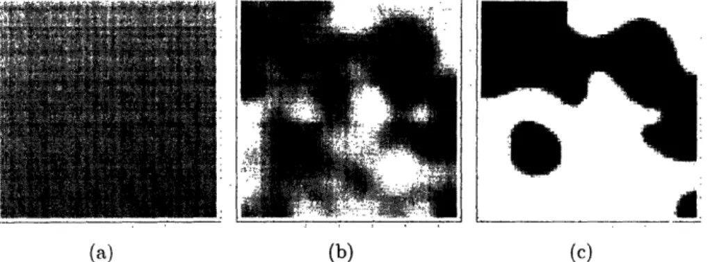
3-1 Images displaying the progress of a composition field evolving via the

Allen-Cahn equation. The grey field (a) shows the initial conditions at t = 0 in an unstable state. (b) Shows the evolution at t = 1.25 and (c) is at t = 4 where the composition has clearly decomposed into separate phases. ... 18

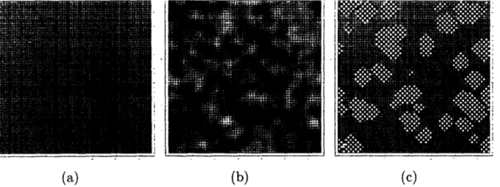
4-1 Images displaying the progress of a composition field evolving via the Cahn-Hilliard equation combined with the LAX/leapfrog differencing scheme. The grey field (a) shows the initial conditions at t = 0 in an

unstable state. (b) Shows the evolution at t = 1.4 and (c) is at t = 4 where the scheme has clearly become unstable. ... 22

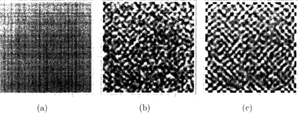
4-2 Images displaying the progress of a composition field evolving via the

Cahn-Hilliard equation combined with the Crank-Nicholson differenc-ing scheme. The grey field (a) shows the initial conditions at t = 0 in an unstable state. (b) Shows the evolution at t = 1.8 and (c) is at

t = 6.0002 where the scheme has clearly become unstable. The errors

along the edges are explained further in 6.2.2. ... 23

4-3 Image displaying the progress of a composition field evolving via the

Cahn-Hilliard equation. The data was first evolved using the LAX/leapfrog nethod until t = 1.4 and then the Crank-Nicholson method was used until t = 6.2 ... ... ... 23

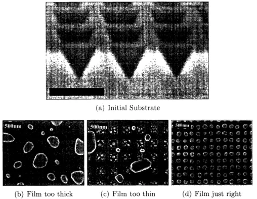
5-1 Imnages displaying the initial substrate (a) and the varying

morpholo-gies reached by the dewetting process due to initial film thickness (b),(c), and (d) (Images courtesy of Amanda L. Giermann ... 26 5-2 Images showing the height above an individual pit from a top down

view where black is 0. It can be seen that for a thick film (a) the rupture points are the four midpoint of each side of the outer box of

the pit. For a thin film (b) however, the rupture points are at the eight bulbous black spots closer to the corners of the outer box of the pit. . 27

5-3 Image of a cross section of the center of a pit. Initial film height was

thin and the secondary rupture points can be seen in the lower sections of either side of the pit ... 27 6-1 Image representing the instabilities of the Crank-Nicholson method used 30

Chapter 1

Introduction

Phase field modeling is an emergent crucial topic for the advancement of material

science research through computer simulations [1, 4, 19, 15, 13, 16, 8, 23]. The nature

of the model itself allows for the simulation of a broad range of binary phase systems such as spinodal decomposition, solid-solid phase transformations, grain boundary

motion, martensitic transformations, etc [21, 1, 4, 19, 15, 13, 16, 8, 231. When the

proper phase equations are coupled with an efficient differencing scheme, the phase

field model presents an expansive set of results which can stimulate deeper

compre-hension of the system at hand.

The choice of a differencing scheme that compliments the evolution equations and can give accurate results within a reasonable time frame is of utmost importance. What we look for is a way to treat separate terms of the phase field equations with separate numerical algorithms to produce results in the most efficient way possible. Operator splitting (sometimes called time splitting) is the method of treating

indi-vidual terms of a PDE with separate differencing schemes and is commonly used

especially when working with an equation that has both linear and nonlinear terms

[9, 14, 12].

It is our initiative to model the Allen-Cahn and Cahn-Hilliard equations (see 2.1) by treating the terms separately and combining effective differencing algorithms.

Ad(litionallv we would like to investigate the methods bv which specific algorithms ob)tain their stability properties when combined and present a friamework for which

these met hods could be replicated.

Section II covers the theoretical background of the Allen-Cahn and Ca.hn-Hilliard equations. The case of modeling the these equations separately is then developed and presellted with relevant data. This is followed by a further investigation of the fourth order spectral methods derived and its application to modeling metallic films evolving

under surface diffusion. We conclude with an overall critique of each algorithm and

Chapter 2

Theoretical Background

2.1 Conservative and Nonconservative Fields

There are two main types of phase field models which are differentiated by the

fun-damental way in which the system is driven into equilibrium. These are considered to be conservative and nonconservative fields [21].

The difference between the two is that a conservative field approaches equilibrium by diffusing material' into local energy minimums, and as such must maintain a constant overall composition at all times [5, 21, 2]. This means that long range

interactions are eventually considered by the model before it reaches equilibrium. On

the other hand, a nonconservative field drives toward equilibrium by processes that don't consider the overall spatial interactions, and can result in varying total phase

fractions as time progresses [21, 5].

In the discrete model created, an image2 was iterated through time based on generalized forms of the Allen-Cahn and Cahn-Hilliard equations

1The use of the word material is understood to mean the net amount of a material parameter in the system. In some cases this can refer to a short range order parameter or another similar ideal measurement

2_{We define an image as a two dimensional matrix of values Cj ranging from 0 to 1 where i and}

j are the indices and n is the index in time. It is convenient to think of the data set in our model as

being an image because the results presented in Chapters 3. 4 and 5 are all visual representations of the data as evolved by the algorithms introduced. Additionally, results will be represented as

grayscale images where illstal)le comll)ositions are rel)resellte( l)y levels of grey, and black and white

c

F + V2C

(2.1)

at OC'

and

DC

at= v Oc - v

C

(2.2)

F(C) = 16C2(C - 1)2 (2.3)

where C represents a composition field. In our simulations, the initial composition fields were all taken to be .5 with random thermal fluctuations on the order of 10-8.

The equations were idealized to avoid modeling any one specific system and to show

the applicability of the methods derived.

2.2 Operator Splitting

Operator splitting is the method by which an equation of the form

Ou

= Lu (2.4)

at

where L is a linear sum of operators, can be solved by independent differencing

schemes for each operator in L [20, 14]. In other words, if your initial value equation

has multiple terms, each one can be modeled by a separate method. The main benefit of this is that the stability criterion becomes that of whichever method is least stable rather than the stability of both terms combined together.

For each term in L = L1 + L2+ ... + Lm the respective differencing algorithm

only acts on the image for A. In this respect. the simulation iterates through time alternating between competing processes. It has been previously shown that this approach to modeling multi-term equations is stable for any t as long as At is the

Chapter 3

Modeling The Allen-Cahn

Equation

The two terms in equation (2.1) are treated separately and subsequently the entire model presented is accurate on first order time scales. This is due to the ability to model the second term via spectral methods which are unconditionally stable [14]. This condition makes the stability solely dependant on the method used for the first term.

3.1 The Interfacial Term

The interfacial energy term in the case of Allen-Cahn depends only on the equation for a. Looking at equation (2.1), it is apparent that the differencing of composition

in time changes based on where the composition lies along the double welled energy

curve in equation (2.3). It is clear then that the algorithm used to forward difference

this part of the equation does not need to be complex as the energy F for any

composition is already known.

With this knowledge, a first order implicit technique was chosen that involves only

cn+l

_{i. = Cj +}

AtF'(C"j)

1 + XtF"(C7ij) (3.1)

and is stable at time steps on the order of 10-1.

3.2 The Diffusive Term

It has been shown that one of the most efficient methods to model an equation of the

form

= -V 2_C

(3.2)

ot

is by the use of Fourier transforms[9, 7]. Discrete Fourier Cosine Transforms (DFCT) were chosen because they only deal with real values, they impose periodic

boundary conditions, and they lead to less overall calculations and memory usage to get an equivalent solution[22]. Essentially the benefit of solving this problem

in frequency space is that you convert a spatial derivative into multiplication by a coefficient [3]. In Fourier space, equation (3.2) is transformed into

=

DC

at

where D is a linear coefficient, and the solution takes the form

C = Cexp DAt (3.4)

To understand better why this method works so well, it is vital to understand how the Fourier transform works. The DFCT

N-I

N-1

H)CC,

I(2n +

1)k

:k

X(k)ZCicos

2N 1)k

=0,1.N-1

i--0

for = ()0,

X(k) =

(3.6)

{

for k=

1,2 ...

.. N-

1

such that k is the index in Fourier space and i is the index in time space from 0

to N - 1. Equation (3.5) reorganizes the information contained in an original image

[22]. Looking at equation (3.5) we can see that each discrete point C(k) in k space

is dependant upon the overlap of a cosine wave with every point C(n) in time space. Essentially the DFCT rearranges the information such that the data describing sharp features is placed further away from the index k = 0. That being said, it is the fact that equation (3.2) tends to drive small perturbations to zero that we can see the convenience of transforming the data [5].

The discrete form of the Laplacian operator

1

V2F ~ x(Fi+ - 2F +

Fi_

)

(3.7)

can be combined with equation (3.5) to find the coefficient D in equation (3.4).

Simplifying the result gives

D(k) = -2

(- 1) )

(3.8)

where k is the index in frequency space. It has been shown that this method is

unconditionally stable and thus it is an ideal method for the Allen-Cahn equation [9]. Additionally it is important to note that because the DFCT is separable, it is applied to an image first on its rows and then on its columns[22]. Due to the fact that it is applied twice, the algorithm that forward differences the composition field must multiply by the solution twice in Fourier space in the following manner

-k''+2' = Cklnk2 exp (D(ki)At) exp (D(kJ)At) (3.9)

(a) (b) (c)

Figure 3-1: Images displaying the progress of a composition field evolving via the

Allen-Cahn equation. The grey field (a) shows the initial conditions at t = 0 in an unstable state. (b) Shows the evolution at t = 1.25 and (c) is at t = 4 where the composition has clearly decomposed into separate phases.

3.3 Results

Due to the relative stability of both numerical algorithms, results for a system that starts at an average composition of .5 with small perturbations on the order of 10- s

can be driven into equilibrium on a timescale on the order of 10 minutes. The

ac-tual time it takes is highly dependant on the environment in which the algorithm is running. The code representing the schemes described running in Mathematica 5.2, a relatively slow environment, took about 3 minutes.

Figure 3-1 shows the evolution of the Allen-Cahn simulation. At the intermediate step the phases are trying to separate due to the interfacial energy, while they are also diffusing together. The final state is a binary phase system with a smooth interface that compares with previous work [2]. It is important to note that though our simulation is not meant to represent any one specific system, through changes in the interfacial energy 9F it is possible to produce more realistic results.

Chapter 4

Modeling The Cahn-Hilliard

Equation

The two terms in equation 2.2 are more complicated than in the Allen-Cahn equation. As such, it was necessary to try multiple differencing algorithms to find the most

efficient one. Finding a stable method to model -V 4C proved easy by following

similar steps to that of the second order case, however the first efforts to model 2_{a__}

proved to be highly unstable.

Both of the following two algorithms used to model V2_{9F use operator splitting}

as well. This is implemented because the Laplacian implies a spatial derivative, but calculation time is saved if the system is differenced in one dimension at a time. Accordingly, the following algorithms treat the Laplacian as if it only applies to rows

of the image, and then as if it only applies to columns of the image. The time step is

halved as described bv section 2.2. The next sections present the methods which did

4.1 The Nonlinear Term

4.1.1

The LAX/Leapfrog Method

As mentioned previously, our first attempts to find a stable differencing algorithm to model the first term of equation (2.2) were unsuccessful. The difficult part was that

_,9 itself is nonlinear and taking the Laplacian of it in space limits the stability. This

is generally due to the mathematical dependance on spatial information and the time it takes before any point Ciljl "knows" about any other point Ci2,j2 where ii >> i2

and j >> j2[20].

The staggered leapfrog method has been shown to be second-order accurate in space and time [20]. Essentially the algorithm involves centering the values at time t by their respective neighbors at times t + At and t - At. This method proves to be stable only for small gradients between data, which will be significant later to help understand why the algorithm fails.

The LAX method is a way to fix the instabilities in the forward time centered Euler scheme [20]. It involves replacing all occurrences of the value at time t position

i with an average of the points at positions i + 1 and i - 1. The reason this increases

stability is the reason the leapfrog scheme tends to fail; each point "knows" about other points around it sooner than it would without the method.

For the first term in equation (2.2) the LAX/leapfrog scheme in one dimension becomes

Ct+1C/n-x--

A2

-

where Ax = 1 in our model. This method can be used with At = i- on all

4.1.2 The Crank-Nicholson With Linearization Method

The Crallk-Nicholson algorithm is intendle(l to l)e second order stable in both space

an(l time while retaining stability and accuracy[20]. This is accomplished by taking

an average between a fully implicit solution and an explicit solution. For the first term. this looks like

i =

Dt F (C+

1

)

-

2F'(C"+')

+

F'( )

(4.2)

C"+1 - C = 2(Ax)2

[

(4.2)

where D is an arbitrary coefficient and Ax = 1 in this model. Using the

lineariza-tion

F'(Cn+) F'(Cn) + F"(Cn) (Cn+1 - C) (4.3)

on equation (4.2) and rearranging the terms yields an easily solveable tridiagonal matrix.

Technically this scheme should be stable for any size At[20]. The results of

simu-lations using this method turned out to be stable only up to At - 10- 4 however, and

the analysis of what went wrong is left to section 6.2.2.

4.2 The Fourth Order Term

For the fourth order term in equation (2.2) we take a similar approach as that in section 3.2. We start with the discrete form of the fourth order derivative

V4_{F Ax}2_{(Fi+2 - 4Fi+l + 6F - 4Fi_}

1 + Fi-2) (4.4)

and then apply equation (3.5) to it. In this case, the resulting coefficient is

D(k) =-16 sin (( 1) (4.5)

2(

i.g is forward diffre via. t1)t as that in section 3.2 and

(a) (b)

Figure 4-1: Images displaying the progress of a composition field evolving via the

Cahn-Hilliard equation combined with the LAX/leapfrog differencing scheme. The grey field (a) shows the initial conditions at t = 0 in an unstable state. (b) Shows the evolution at t = 1.4 and (c) is at t = 4 where the scheme has clearly become unstable.

is again unconditionally stable. This method worked so well in fact, that Chapter 5 goes on to show its application in other fields.

4.3 Results

The LAX/leapfrog method was able to drive the system into its first meta-state1 with relative ease, but quickly became unstable when the gradients became larger as predicted.

Figure 4-1 illustrates the known nature of the leapfrog method [20]. It is able to quickly drive the system accurately, but eventually it becomes unstable and the result is useless. Starting from an initial state and using the Crank-Nicholson scheme generates a similar initial result as shown in Figure 4-2, however the method turned out to be unstable as well. There are several reasons that could cause the errors in the Crank-Nicholson simulations, and they are examined in section 6.2.2.

Figure 4-3 displays the only result that compares to known images of spinodal decomposition. This image was produced by taking the data from the LAX/leapfrog mletho(l before it becomes unstable, and then switching to the Crank-Nicholson

algo-rithli. Though it appears to be an indication of a valid method, section 6.2.2 explains

(a) (b)

Figure 4-2: Images displaying the progress of a composition field evolving via the Cahn-Hilliard equation combined with the Crank-Nicholson differencing scheme. The

grey field (a) shows the initial conditions at t = 0 in an unstable state. (b) Shows the evolution at t = 1.8 and (c) is at t = 6.0002 where the scheme has clearly become

unstable. The errors along the edges are explained further in 6.2.2.

Figure 4-3: Image displaying the progress of a composition field evolving via the

Cahn-Hilliard equation. The data was first evolved using the LAX/leapfrog method until t = 1.4 and then the Crank-Nicholson method was used until t = 6.2

further.

Chapter 5

Modeling Dewetting Due to

Surface Diffusion

5.1 Theoretical Background

To show the validity of the spectral method proposed in section 4.2 a model was

con-structed to simulate the surface diffusion dewetting of a metallic film on a substrate. The problem is currently being studied as a means to create an array of monodisperse

nanoparticles [10, 11]. It has been shown that when a substrate such as in Figure

5-1(a) is coated with an ideal thickness of metallic film and subject to the right heating

conditions, surface diffusion will drive material to form a single nanoparticle in each

pit. The results vary as the initial thickness ho diverges from the ideal however, and the consequent equilibrium states are displayed in Figures 5-1(b-d).

Depending on the boundary conditions and initial geometry of the system chosen the film evolves into exceedingly dissimilar equilibrium states. It is theorized that the cause of this might be due to the point (in both time and space) at which tile substrate ruptures the surface of the film [10]. When this occurs, the dynamics are

no longer defined by surface diffusion alone, but an additional interfacial energy is

(a) Initial Substrate

(b) Film too thick (c) Film too thin (d) Film just right

Figure 5-1: Images displaying the initial substrate (a) and the varying morphologies reached by the dewetting process due to initial film thickness (b),(c), and (d) (Images courtesy of Amanda L. Giermann.

Oh

At

_V

4

h

(5.1)

at

where h is the height above the substrate.

It is clear then that using the algorithm presented in section 3.2, the construct

for this simulation is already complete. In this case the image is no longer composed of values ranging from zero to one, but from values that represent the height of the film. Defining the initial geometry as exhibited in experiments is relatively simple,

and an efficient model is created that can easily drive the system to determine both how long it takes for the substrate to rupture the surface and where it does this dleending on the initial conditions. The following section presents the approach to varying the initial conditions followed by a analysis of the results and how they

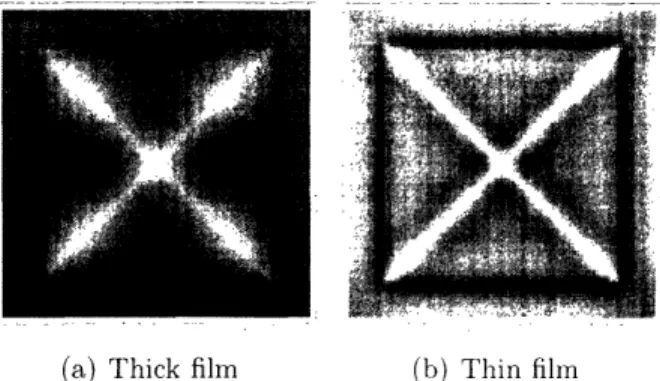
(a) Thick film (b) Thin film

Figure 5-2: Images showing the height above an individual pit from a top down view where black is 0. It can be seen that for a thick film (a) the rupture points are the four midpoint of each side of the outer box of the pit. For a thin film (b) however,

the rupture points are at the eight bulbous black spots closer to the corners of the outer box of the pit.

".::: ::: ;. ::":....: ~t t i ~~~~~~i Sll, ,,I t s ''~

~ ~~~~~.

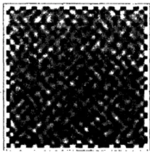
Figure 5-3: Image of a cross section of the center of a pit. Initial film height was thin

and the secondary rupture points can be seen in the lower sections of either side of the pit.

5.2 Results

The model was efficient enough that results for a wide rangfe of initial geometries could be determined in less than a minute. ost interesting was the fact that as the

film egan to get too thin, the rupture points moved as shown in Figure 5-2.

Tills implies in part an explanation of the reslts found in lab (Figure 5-1). Taking

the result of the thin film further in the simulation, Figure 5-3 shows that the next polits to rpture the surface aside from the outer rim C aae the four dark spots around the center of the ottom of the pit i Figure 5-2(). Tluis will be atnalyzed in section

6.3-.

I -1

Chapter 6

Analysis

6.1 Operator Splitting

As defined, operator splitting is a stable method when individual operator stability conditions are met [14, 20]. What is unclear however is what sort of results arise when separate operators are working against each other (such as those in Figure 4-2(c)).

The two terms in equation (2.2) are opposing processes. One tends to drive the system into binary phases as the other pushes the system into a state of an average composition. There must be some balance between the terms that is independent of the method by which they are modeled, however this balance is dependant on the relation between the fundamental processes and the math that describes them.

It is obvious from evolution of the Cahn-Hilliard model that at time t = 0 the interfacial energy term drives the system quickly into separate meta phases. It appears from the data however, that once the relative compositions are no longer in the

f"(C(xi,j)) < 0 range, they aren't changing fast enough to counteract the changes

made by the second term. 1 From here they are slowly smoothed out until an overall

ordered distribution of phases is formed. Though time was a limiting factor, the approach to the final state can be seen in Figure 6-1. Note the formation of regions of alternating phase and the distinct angular nature of what would otherwise be the

1_{Assulllilg ta.t. the imltroper behavior displayed is not cluse(l by) the decision to lineaize the}

Figure 6-1: Image representing the instabilities of the Crank-Nicholson method used spinodal. This appears to be the point at which the two terms will balance, and the system will be at equilibrium once the full image is similar to the edges. This is not

a desired feature, yet it calls for some thought as it is fundamentally possible for a

real system to have a mobility large enough to compete with the interfacial energy. The programming of the algorithm cannot be completely at fault however because the image evolves properly early on. Therefor it is likely that there is some unknown process governing the evolution of this system, and it requires further investigation. Though it was unclear what caused the Crank-Nicholson method to fail in these simulations, the result should not be treated as trivial. Additionally there must be something wrong with the periodic boundary conditions as they appear to be causing

instabilities at the edges.

6.2 Phase Field Models

6.2.1

The Allen-Cahn Model

The proposed Allen-Cahn model works efficiently for simulating non-conservative phase fields. Though it is not necessary to make the algorithm any more efficient, it is important to note that the interfacial energy term is not always ideally modeled by an implicit method. Should the interfacial energy be dependant upon some other function, the scheme may have taken on a different approach. A Runge-Kuttah method might be usefiul for particular systems, as well as a method of variable time

alteration algorithm can boost a simulations performance greatly [20]. Our sinmulation didl not require any such method, but if the image was on the order of 106 grid points

or larger, it would have been useful.

6.2.2

The Cahn-Hilliard Model

The Cahn-Hilliard model was overall unsuccessful, partially due to time constraints. It did however produce interesting results which need further investigation. Further-more, the one method that did work (using LAX/leapfrog and then Crank-Nicholson) suggests a different approach to modeling. Though operator splitting is a commonly used practice, choosing an algorithm at different times throughout the evolution of the system based on the morphology is just as useful. Especially with a scheme such

as LAX/leapfrog which is only stable for small gradients, more efficient approaches

to phase field modeling are still yet to be discovered.

As mentioned before, it is unlikely that the instabilities in the Crank-Nicholson algorithm are due to a trivial error. Perhaps this result does in fact have some potential as a useful reference. Further efforts to run this simulation at smaller time steps may prove to generate a more valid result, yet the evolution does not appear to change as the time step goes from 10-3 to 10-6. Whether or not the instabilities arise from a mathematical error, the approach to modeling non-linear terms must always be considered thoroughly. An additional effort was made to attempt to take the DFCT of equation (2.3). For the interfacial energy used, this proved to be a non-algebraic solution. When the interfacial energy was linearized and then used with the DFCT, a proper solution was still not acquired as there was a ± term without any

way to determine which solution to use in Fourier Space. There are likely forms of the interfacial energy however. that when transformed can be solved in Fourier space to provide a spectral solution to a non-linear terml.

6.3 Dewetting Model

The results of the dewetting model present extremely useful concepts. The result of having the film too thick in the simulation does not present anything that could explain what is seen in Figure 5-1(b). Rather, this process seems to be random and could possibly be modeled if the simulation were adjusted to include thermal fluctuations and the interfacial energy that occurs after the substrate breaks through. Most interesting was the realization that at small initial film heights the substrate does not break through at the centers of each pit face. Additionally, the next parts of the surface to break through are the four spots shown in Figure 5-3 and comparing this to Figure 5-2(b) it seems to explain the production of many polydisperse nanoparticles in the pits. Even more convincing that this is what actually occurs is that in Figure 5-1(c) the average amount of particles in each pit is five. If the substrate ruptures the surface of the film inside the pit evenly at the four points shown and the ruptures and subsequent interfacial energies are what cause individual particles to form, then the model appears to explain what is found in lab.

The dewetting simulation proved to be highly stable and through changes to the initial conditions new insights were discovered. This is just one application of this method to a very specific system, but further research will surely prove beneficial using the spectral techniques derived. One caveat is that the integral of the surface through time shows a slight increase in mass. Though this was not treated in these simulations, there are specific measures to prevent mass fluctuations outlined by previous work

Chapter 7

Conclusions and Further Research

This work was carried out to investigate the method of splitting operators in phase

field equations in order to model systems in an efficient and effective way. The

differencing schemes developed were used to generate data that compared well with previous attempts. Though the Cahn-Hilliard model was not completely effective, it gives rise to relevant questions about the nature in which competing processes work in a binary phase system. The Allen-Cahn model outlined is highly applicable to many phase field systems and could be employed in many future studies. Possibly even more applicable is the fourth order spectral method developed which has shown to be extremely effective in modeling surface diffusion.

More work must be done to determine the failure of the Cahn-Hilliard model presented in Chapter 4. Clearly there is a problem with the periodic boundary con-ditions as well as the fighting processes between the split operators. Furthermore, the fundamentals of operator splitting has not been heavily studied, and it certainly requires a mathematical analysis which is capable of describing the way that specific operators will interact with each other. Doing this will provide great insight into the nature of the phase field equations as well as many other systems. A formal basis

on which the terms in any equation can be conlpared as competing processes would

provide a starting point for approaching any simulation.

Further study of the usefulness of spectral methods is essential. Any system that involves a second or fourth order gradielt term could )enefit fiom the schemes

outlined in Chapters 3 and 4. Additionally, the dlewetting problem can be simulated

for nearly any initial geometry and thus presents a. method by which new uses of the

dewetting process can be derived.

An interesting study would be to use the Discrete Laplace Transform to impose asymmetric boundary conditions on an evolving system. Via a similar method as that in section 4.2, the DLT could use unit step functions to define a geometry and

forward difference a non-rectangular composition field. This could give rise to new

implications toward real lab work, and would be relatively computationally

Bibliography

[1] A. Artemev, Y. Jin, and A. G. Khachaturyan. Three-dimensional phase field

model of proper martensitic transformation. Acta Materialia, 49(7):1165--1177, 2001.

[2] Robert W. Balluffi, Samuel M. Allen, and W. Craig Carter. Kinetics of Materials.

John Wiley & Sons, Inc., 2005.

[3] R. J. Beerends, H. G. ter Morsche, J. C. van den Berg, and E. M. va de Vrie.

Fourier and Laplace Transforms. Cambridge University Press, Cambridge, 2003.

[4] J. W. Cahn, P. Fife, and 0. Penrose. A phase-field model for diffusion-induced

grain-boundary motion. Acta Materialia, 45(10):4397-441, 1997.

[5] W. Craig Carter, J. E. Taylor, and J. W. Cahn. Variational methods for mi-crostructural evolution. J. Minerals Metals Mater: Soc, 49(12):30-36, 1998. [6] C. L. Chang and John J. Nelson. Least-squares finite element method for the

stokes problem with zero residual of mass conservation. Society for Industrial

and Applied Mathematics Numerical Analysis, 34(2):480-489, 1997.

[7] L. Q. Chen and J. Shen. Applications of semi-implicit fourier-spectral method

to pha-se field equations. Computer Physics Communications, 108(2):147-158, 1998.

[8] Zhiinilg Chen and K. H. Hoffman. An error estimate for a finite-element scheme for a l)ha.se field model. IMA Journal of Numerical Analysis. 14(2):243--255,

[9] L. O. Eastgate. J. P. Sethila, i. . Rauscher. T. Cretegny. C. S. Chen. and C. R.. yIvers. Phys. Rev. E, 65(3). 2002.

[10] Amanda L. Gierrnann and Carl V. Thompson. Solid-state dlewetting for ordered arrays of crystallographically oriented metal particles. Applied Physics Letters,

86(12), 2005.

[11] Amanda L. Giermann, Carl V. Thompson, and Henry I. Smith. Templated formation of ordered metallic nano-particle arrays. Nanoparticles and Nanowire

Building BlocksSynthesis, Processing, Characterization and Theory, 818:37-42,

2004.

[12] Helge Holden, Kenneth Hvistendahl Karlsen, and Knut-Andreas Lie.

Computa-tional Geosciences, 4:287-322, 200.

[13] D. Jacqmin. Calculation of two-phase navierstokes flows using phase-field mod-eling. Journal of Computational Physics, 155(1):96-127, 1999.

[14] Kenneth Hvistendahl Karlsen and Nils Henrik Risebro. An operator splitting method for nonlinear convection-diffusion equations. Numerische Mathematik,

77(3):365-382, 1997.

[15] Alain Karma. Phase-field model of eutectic growth. Physical Review E,

49:2245-2250, 1994.

[16] Alain Karma and W. J. Rappel. Physical Review E, 57(1):4323-4349, 1998.

[17] Joachim Krug, Michael Plischke, and Martin Siegert. Surface diffusion currents

and the universality classes of growth. Physical Review Letters, 70:3271--3274, 1993.

[18] Z. W. Lai and S. Das Sarma. Kinetic growth with surface relaxation: Continuum

versus atomistic models. Physical Review Letters, 66:2348--2351, 1991.

[2()] William H. Press. Sa-ul A. Teukolsky, William T. Vetterling, and Brian P.

Flan-nery. lumerical Recipes irn C. Cambridge University Press, second edition. 1992. [21] Dierk Raabe, Franz Roters. Frdric Barlat, and Long-Qing Chen, editors.

Con-tinuum Scale Simulation of Engineering Materials. Wiley-VCH Verlag GmbH &

Co. KGaA, 2004.

[22] D. Sundararajan. The Discrete Fourier Transform Theory, Algorithms and

Ap-plications. World Scientific Publishing Co. Pte. Ltd., 2001.

[23] A. A. Wheeler, G. B. McFadden, and W. J. Boettinger. Mathematical, Physical