HAL Id: hal-00677063
https://hal.archives-ouvertes.fr/hal-00677063
Submitted on 19 Feb 2013HAL is a multi-disciplinary open access
archive for the deposit and dissemination of sci-entific research documents, whether they are pub-lished or not. The documents may come from teaching and research institutions in France or abroad, or from public or private research centers.
L’archive ouverte pluridisciplinaire HAL, est destinée au dépôt et à la diffusion de documents scientifiques de niveau recherche, publiés ou non, émanant des établissements d’enseignement et de recherche français ou étrangers, des laboratoires publics ou privés.
Analyzing the dynamic response of a rotor system under
uncertain parameters by Polynomial Chaos Expansion
Jérôme Didier, Béatrice Faverjon, Jean-Jacques Sinou
To cite this version:
Jérôme Didier, Béatrice Faverjon, Jean-Jacques Sinou. Analyzing the dynamic response of a rotor sys-tem under uncertain parameters by Polynomial Chaos Expansion. Journal of Vibration and Control, SAGE Publications, 2012, 18 (5), pp.587-607. �10.1177/1077546311404269�. �hal-00677063�
Analyzing the dynamic response of a rotor system
under uncertain parameters by Polynomial Chaos
Expansion
Jérôme Didiera, Béatrice Faverjonb and Jean-Jacques Sinoua
aLaboratoire de Tribologie et Dynamique des Systèmes UMR-CNRS 5513
Ecole Centrale de Lyon, 36 avenue Guy de Collongue 69134 Ecully Cedex, France
email: jean-jacques.sinou@ec-lyon.fr
b Laboratoire de Mécanique des Contacts et des Structures UMR-CNRS 5259
INSA-Lyon, 18-20, rue des Sciences 69621 Villeurbanne Cedex France
Abstract
In this paper, the quantification of uncertainty effects on response variability in rotor systems is investigated. To avoid the use of Monte Carlo simulation (MCS), one of the most straight-forward but computationally expensive tools, an alternative procedure is proposed. Monte Carlo Simulation builds statistics from responses obtained from sampling uncertain inputs by using a large number of runs. However, the method proposed here is based on the stochastic finite element method (SFEM) using polynomial chaos expansion (PCE).
The efficiency and robustness of the method proposed is demonstrated through different nu-merical simulations in order to analyze the random response against uncertain parameters and random excitation to assess its accuracy and calculation time.
Keywords: dynamics, rotor, uncertainties
1
Introduction
In rotordynamics, two types of uncertainty on dynamic systems are of particular interest. The first of these can derive from variations in mechanical properties (such as mass, stiffness and geometrical imperfections) due to manufacturing errors [Lalanne and Ferraris (1990); Friswell and Mottershead (1995); Erich (1992); Childs (1993); Yamamoto and Ishida (2001)]. Besides this type of structural uncertainties, external and internal forcing functions can also be random.
Numerous methods have been used to quantify physical uncertainties in a variety of computational problems like the perturbation method, the Monte Carlo Simulations and the Polynomial Chaos Ex-pansion [Ghanem and Spanos (1991)]. The perturbation method based on the exEx-pansion of random quantities into Taylor series [Nayfeh (1973)] and the Neumann method based on Neumann series
expansion [Benaroya and Rehak (1988); Yamazaki et al. (1988)] provide acceptable results for small random fluctuations, then they are not adapted here for solving a dynamic problem in the case of an excitation frequency close to a resonance frequency. The direct Monte Carlo Simulations, which is the most straightforward and frequently used approach, is adapted to include uncertainties in a determinis-tic finite element model, by generating n independent samples of the random parameter. Then it leads to solve the deterministic problem n times in order to obtain n samples of the response vector and so the statistics of the response. Due to the slow convergence rate of this method, a very high number of samples is necessary then if solving the deterministic problem is already computationally intensive, the computational costs of the method can become impractical. Particularly, rotordynamics problems are quite complex to solve in a deterministic sense. The polynomial chaos expansion associated with a Galerkin projection so-called stochastic finite element method [Ghanem and Spanos (1991)] has shown to be a successful approach to solve uncertainty quantification problems. It represents the stochastic processes and variables in a set of orthogonal bases of random variables. The polynomial chaoses are from the homogeneous chaos theory of Wiener [Wiener (1938)] and the original poly-nomial chaos expansion [Ghanem and Spanos (1991)] used a mean-square convergent expansion as multidimensional Hermite polynomials of normalized Gaussian variables. Since the Hermite poly-nomials are orthogonal with respect to the Gaussian measure, the homogeneous polynomial chaos can achieve optimal exponential convergence for Gaussian inputs [Ghanem (1999)]. This last method then seems the most adapted to study the influence of the uncertainties on the parameters of the rotor structure on the response.
The present paper is organized as follows: firstly, we present the rotor system after which a brief explanation is given of the Stochastic Finite Element Method [Ghanem and Spanos (1991)] for the solution of mechanical problems with several random characteristics. Secondly, expansions of the operator of random material properties and of the random external forcing function on the chaos ba-sis are explained and studied for application to the rotordynamics problem. The Polynomial Chaos Expansion procedure is illustrated by different numerical examples that include the most common sources of randomness in a rotordynamics problem (such as physical and geometric parameters). Thirdly, the results obtained by applying the Polynomial Chaos Expansion (PCE) procedure are com-pared with those evaluated by Monte Carlo Simulation (MCS) whose costs become prohibitive for large finite element models with large numbers of design parameters. Finally, the efficiency and ro-bustness of the method proposed is demonstrated through several numerical simulations of the effects of uncertainties and orders of polynomial chaos.
2
Rotor Model
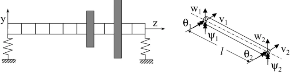
The system under study is illustrated in Figure 1. The rotor consists of a rotor shaft with two discs. The shaft is discretized into 10 Timoshenko beam finite elements with four degrees of freedom at each node [Lalanne and Ferraris (1990); Friswell and Mottershead (1995)] and a constant circular section. All the values of the parameters are given in Table 1. The beam element model is given by
[Me]{ ¨
xe} + ([Ce] + ω[Ge]){ ˙
xe} + [Ke]{xe} = {qe}
where the vector{qe} defines forces applied on the shaft and ω is the rotational speed of the shaft.
[Me] and [Ge] are the mass and gyroscopic matrices of the shaft element. [Ke] and [Ce] are the
elementary stiffness and damping matrices. These matrices are described in A. The model of the rigid discs is given by
[Md]{ ¨xd} + ω[Gd]{ ˙xd} = {qd} (2)
where[Md] and [Gd] are the mass and gyroscopic matrices of the disc. These matrices will be
de-scribed in the following part of the paper. The vector {qd} defines the unbalance forces due to an
eccentric mass. For the degree-of-freedom [v w θ ψ]T (see Figure 1), the unbalance forces are
given by qd= [medeω 2 cos(ωt + φ) medeω 2 sin(ωt + φ) 0 0]T (3)
where meand deare the mass unbalance and the eccentricity respectively. φ and ω define the initial
angular position in relation to the z-axis and the rotational speed of the rotor. Finally, discrete stiffness components are located at either end of the shaft. After assembling the shaft elements and the rigid discs, the equation of motion for the complete rotor system is defined as follows:
[M] ¨{x} + ([C] + ω[G]) ˙{x} + ([K] + [Kb]){x} = {q} (4)
where[M] and [G] are the mass and gyroscopic matrices of the shaft and the two discs. [K] and [C] are
the stiffness and damping matrices of the shaft.[Kb] is the stiffness matrix of the bearings. {q} is the
unbalance forces of the complete rotor system. Considering that the unbalance force can be written as{q} = {Q}eiωt, the response vector may be assumed to be{x} = {X}eiωt. By using Equation (4),
the system governing the equation in the frequency domain is given by
[A(ω)]{X(ω)} = {Q(ω)} (5) where
[A(ω)] = −ω2
[M] + iω([C] + ω[G]) + [K] + [Kb] (6)
In the following part of the paper, the frequency dependence will be omitted to simplify the notation and[A(ω)] will be noted as [A].
3
Stochastic model
In rotordynamics, uncertainties on dynamic responses can occur due to manufacturing inaccuracies related to mechanical properties such as mass, stiffness, damping and geometrical imperfections. Moreover, forcing functions (external and internal) also lead to considerable uncertainties, so that
they have to be taken as random quantities. Therefore, considering in this part [A], {X} and {Q} as
random processes, where argument τ denotes the random character, Equation (5) can then be rewritten in a random way such that
Figure 1: Rotor system and Shaft finite element
Material and geometrical properties are randomly modeled by [M(τ )], [G(τ )], [K(τ )], [C(τ )] and
[Kb(τ )], thus Equation (6) becomes
[A(τ )] = −ω2
[M(τ )] + iω([C(τ )] + ω[G(τ )]) + [K(τ )] + [Kb(τ )] (8)
3.1
The system equation on the Polynomial Chaos basis
The Polynomial Chaos basis is a set of orthogonal bases of random variables, represented in a mean-square convergent expansion by multidimensional Hermite polynomials of normalized Gaussian vari-ables. A rapid overview on the construction of the basis is given below and more details can be found in [Ghanem and Spanos (1991)]. In the following of the paper, the random behavior of each physical or geometrical quantity M (scalar or matrix) considered would be sufficiently modeled by using the Karhunen-Loeve expansion implemented in the Galerkin formulation of the finite element method [Ghanem and Spanos (1991)], then we can expand M such as
M= M +
L
X
l=1
ξlMl (9)
where {ξ1, ...ξL} is a set of orthonormal random variables, M is the mean of M and Ml is its lth
expansion term. The response can be expanded on the Polynomial Chaos basis such that
{X(τ )} =
∞
X
j=0
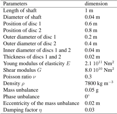
Parameters dimension
Length of shaft 1 m
Diameter of shaft 0.04 m
Position of disc 1 0.6 m
Position of disc 2 0.8 m
Outer diameter of disc 1 0.2 m
Outer diameter of disc 2 0.4 m
Inner diameter of discs 1 and 2 0.04 m
Thickness of discs 1 and 2 0.02 m
Young modulus of elasticity E 2.11011
Nm2 Shear modulus G 8.01010 Nm2 Poisson ratio ν 0.3 Density ρ 7800 kg m−3 Mass unbalance 0.05 g Phase unbalance 0◦
Eccentricity of the mass unbalance 0.02 m
Damping factor η 0.03
Table 1: Model parameters
whereΨj(ξ(τ )) refers to a rearrangement of the p-order finite dimensional orthogonal polynomials
in relation to the Gaussian function that forms a complete basis in the space of second-order random
variables ; {X}j is the unknown deterministic jth vector associated with Ψj(ξ(τ )) and ξ = {ξr}
[Ghanem and Spanos (1991)]. Finally, the system to be solved, when expanded on the polynomial chaos basis, is
∞
X
j=0
[A(τ )]{X}jΨj(ξ(τ )) = {Q(τ )} (11)
with random quantities[A(τ )] and [Q(τ )] defined by
[A(τ )] = ∞ X i=0 [A]iΨi(ξ(τ )) (12) with [A]i = −ω 2 [ ˆM]i+ iω([ ˆC]i+ ω[ ˆG]i) + [ ˆK]i+ [ ˆKb]i i= 0, 1, ..., ∞ (13) and [Q(τ )] = ∞ X k=0 { ˆQ}kΨk(ξ(τ )) (14)
where quantity ˆQ denotes the rearrangement of quantity Q in the polynomial chaos basis. Details
of the rearrangement will be given in the following section of the paper. It should be noted that each random expansion will be described in Subsection 3.2. Finally, the system to be solved to the
subspace spanned by{Ψk}∞k=0, is ∞ X i=0 [A]iΨi(ξ(τ )) ! ∞ X j=0 {X}jΨj(ξ(τ )) ! = ∞ X k=0 { ˆQ}kΨk(ξ(τ )) (15)
which, after doing a Galerkin projection on the polynomial chaos basis, can also be rewritten as
∞ X i=0 ∞ X j=0
E{ΨiΨjΨk}[A]i{X}j = { ˆQ}kE{Ψ 2
k} k = 0, 1, ..., ∞ (16)
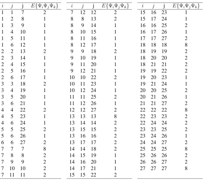
where E{} denotes the operation of mathematical expectation. It should be noted that coefficients
E{ΨiΨjΨk} and E{Ψ 2
k} only have to be calculated once. In practice, the expansion can be truncated
after the P th term where P is the total number of polynomial chaoses used in the expansion excluding the0th order term and can be determined by
P = 1 + p X s=1 1 s! s−1 Y r=0 (L + r) (17)
and in which p is the order of homogeneous chaos used.
3.2
The random quantities in the stochastic rotor
There are different sources of randomness in the rotordynamics problem studied due to geometric and material parameters. This paper deals with uncertainties modeled by Gaussian random variables that represent the random character of the parameters, such as the Young modulus of the shaft, bearing stiffness, disc diameter and density and the amplitude of the unbalance force. All these random quantities are modeled by using expansion defined in Equation (9) and, for physically strictly positive parameters, the random variables of negative values have been removed.
Stiffness of the shaft From the random character of the Young modulus modeled by one truncated
Gaussian random variable ξ1, thus, from expansion described in Equation (9), we obtain the relation
E(τ ) = E(1 + δEξ1) (18)
where E and δE are respectively the mean value and the variation coefficient of the Young modulus.
The detailed deterministic expression of the elementary stiffness matrix of the shaft[Ke] as a function
of the Young modulus is described in A. By introducing the random Young modulus defined above and after assembling the elementary stiffness matrices of the shaft, it is easy to find the random
expansion of[K]
[K] = [K]0+ ξ1[K]1 (19)
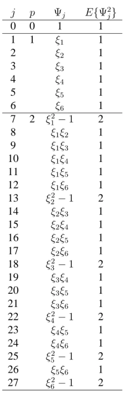
j p Ψj E{Ψ 2 j} 0 0 1 1 1 1 ξ1 1 2 ξ2 1 3 ξ3 1 4 ξ4 1 5 ξ5 1 6 ξ6 1 7 2 ξ2 1 − 1 2 8 ξ1ξ2 1 9 ξ1ξ3 1 10 ξ1ξ4 1 11 ξ1ξ5 1 12 ξ1ξ6 1 13 ξ2 2 − 1 2 14 ξ2ξ3 1 15 ξ2ξ4 1 16 ξ2ξ5 1 17 ξ2ξ6 1 18 ξ2 3 − 1 2 19 ξ3ξ4 1 20 ξ3ξ5 1 21 ξ3ξ6 1 22 ξ2 4 − 1 2 23 ξ4ξ5 1 24 ξ4ξ6 1 25 ξ2 5 − 1 2 26 ξ5ξ6 1 27 ξ2 6 − 1 2
i j j E{ΨiΨjΨk} 1 1 7 2 1 2 8 1 1 3 9 1 1 4 10 1 1 5 11 1 1 6 12 1 2 2 13 2 2 3 14 1 2 4 15 1 2 5 16 1 2 6 17 1 3 3 18 2 3 4 19 1 3 5 20 1 3 6 21 1 4 4 22 2 4 5 23 1 4 6 24 1 5 5 25 2 5 6 26 1 6 6 27 2 7 7 7 8 7 8 8 2 7 9 9 2 7 10 10 2 7 11 11 2 i j j E{ΨiΨjΨk} 7 12 12 2 8 8 13 2 8 9 14 1 8 10 15 1 8 11 16 1 8 12 17 1 9 9 18 2 9 10 19 1 9 11 20 1 9 12 21 1 10 10 22 2 10 11 23 1 10 12 24 1 11 11 25 2 11 12 26 1 12 12 27 2 13 13 13 8 13 14 14 2 13 15 15 2 13 16 16 2 13 17 17 2 14 14 18 2 14 15 19 1 14 16 20 1 14 17 21 1 15 15 22 2 i j j E{ΨiΨjΨk} 15 16 23 1 15 17 24 1 16 16 25 2 16 17 26 1 17 17 27 2 18 18 18 8 18 19 19 2 18 20 20 2 18 21 21 2 19 19 22 2 19 20 23 1 19 21 24 1 20 20 25 2 20 21 26 1 21 21 27 2 22 22 22 8 22 23 23 2 22 24 24 2 23 23 25 2 23 24 26 1 24 24 27 2 25 25 25 8 25 26 26 2 26 26 27 2 27 27 27 8
Table 3: Coefficient E{ΨiΨjΨk}, E{ΨiΨjΨk} = E{ΨjΨiΨk} = E{ΨiΨkΨj}, Six-Dimensional
Similarly, the hysteretic damping is defined by
[Ce] = η
ω[K
e] (21)
where η is the hysteretical damping factor. Assembling elementary damping matrices of the shaft yields:
[C] = [C]0+ ξ1[C]1 (22)
Bearing stiffness For the shaft corresponding to the degree-of-freedom[v w θ ψ]T, the deterministic
elementary stiffness matrix of the bearing is defined as
[Ke b] = k1x 0 0 0 k1y 0 0 0 0 sym 0 (23)
where k1x and k1y are the stiffnesses of the bearing in directions x and y. In this case, it has been
chosen to only investigate the randomness of the stiffness on the first bearing in direction x modeled
by the truncated Gaussian random variable ξ2, which yields:
k1x(τ ) = k1x(1 + δk1xξ2) (24)
in which k1x and δk1x are the mean value and the variation coefficient of the stiffness. Finally, the
expression of the assembled stiffness matrix[Kb] is written as
[Kb] = [Kb]0+ ξ2[Kb]1 (25)
Disc parameters The parameters of the discs should be random. Here, we consider the randomness
on the outer diameter D(τ ) and the density ρ(τ ) of one of the discs, which are the geometric and
material parameters of the model. Describing them by using two truncated Gaussian random variables
ξ3 and ξ4 yields
D(τ ) = D(1 + δDξ3) (26)
ρ(τ ) = ρ(1 + δρξ4) (27)
where D and ρ are the mean values, δD and δρ are the variation coefficients of the diameter and the
density of the disc respectively. These quantities appear in the definition of the mass and gyroscopic
elementary matrices[Md] and [Gd] that are expressed for the disk relative to the degree of freedom
[v w θ ψ]Tsuch that [Md] = md(τ ) 0 0 0 0 md(τ ) 0 0 0 0 Id(τ ) 0 0 0 0 Id(τ ) , [Gd] = 0 0 0 0 0 0 0 0 0 0 0 −Ip(τ ) 0 0 Ip(τ ) 0 (28)
with md(τ ) = 1 4ρ(τ )πh(D(τ ) 2 − d2 ) (29) Id(τ ) = 1 64ρ(τ )πh(D(τ ) 4 − d4 ) + 1 48ρ(τ )πh 3 (D(τ )2− d2 ) (30) Ip(τ ) = 1 32ρ(τ )πh(D(τ ) 4 − d4 ) (31)
in which h and d are the thickness and the inner diameter of the disc respectively. In addition, md is
the mass of the disk. Id and Ip are the diametral moment of inertia about any axis perpendicular to
the rotor axis and the polar moment of inertia about the rotor axis.
Substiting Equations (26-27) in Equations (29) to (31) leads to the expression of the components of the mass and gyroscopic elementary matrices such that
md(τ ) = 4 X j=0 1 X i=0 mdijξ3jξ i 4 Id(τ ) = 4 X j=0 1 X i=0 Idijξ3jξ i 4 Ip(τ ) = 4 X j=0 1 X i=0 Ipijξ3jξ i 4 (32)
where mdij, Idij and Ipij are given in B. The Polynomial Chaos Expansion for md(τ ), Id(τ ) and
Ip(τ ), constructed for two random variables ξ3 and ξ4 is given by
md(τ ) = N X j=0 mdjΨj(ξ3, ξ4) Id(τ ) = N X j=0 IdjΨj(ξ3, ξ4) Ip(τ ) = N X j=0 IpjΨj(ξ3, ξ4) (33)
in which mdij, Idij and Ipij are determined after identification between Equations (32) and (33) using
Tables 4 and 5. The number of polynomial chaoses N is deduced from Equation (17) by two random
variables: L = 2. It should be noted that this identification yields a minimum order p = 5. Then,
expressing mass and gyroscopic elementary matrices of a disc [Md e] and [Gd e] in the polynomial
chaos basis yields
[Md] = P X j=0 [Md]jΨj(ξ3, ξ4) [Gd] = P X j=0 [Gd]jΨj(ξ3, ξ4) (34) where [Md]j = mdj 0 0 0 0 mdj 0 0 0 0 Idj 0 0 0 0 Idj , [Gd]j = 0 0 0 0 0 0 0 0 0 0 0 −Ipj 0 0 Ipj 0 (35)
Finally, the assembled mass and gyroscopic matrices are given by
[M] = P X j=0 [M]jΨj(ξ3, ξ4) and [G] = P X j=0 [G]jΨj(ξ3, ξ4) (36)
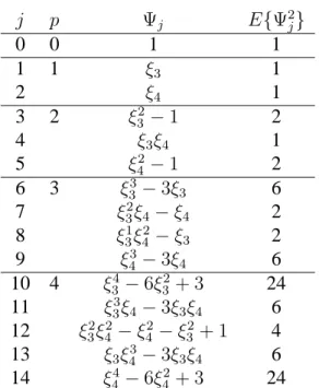
j p Ψj E{Ψ2j} 0 0 1 1 1 1 ξ3 1 2 ξ4 1 3 2 ξ2 3 − 1 2 4 ξ3ξ4 1 5 ξ2 4 − 1 2 6 3 ξ3 3− 3ξ3 6 7 ξ2 3ξ4− ξ4 2 8 ξ1 3ξ 2 4− ξ3 2 9 ξ3 4− 3ξ4 6 10 4 ξ4 3 − 6ξ 2 3 + 3 24 11 ξ3 3ξ4− 3ξ3ξ4 6 12 ξ2 3ξ 2 4 − ξ 2 4 − ξ 2 3 + 1 4 13 ξ3ξ 3 4− 3ξ3ξ4 6 14 ξ4 4 − 6ξ 2 4 + 3 24
Table 4: Two-Dimensionnal Polynomial Chaoses and their variance
1 Ψ0 ξ3 Ψ1 ξ4 Ψ2 ξ2 3 Ψ3+ Ψ0 ξ3ξ4 Ψ4 ξ2 4 Ψ5+ Ψ0 ξ3 3 Ψ6 + 3Ψ1 ξ2 3ξ4 Ψ7+ Ψ2 ξ3ξ 2 4 Ψ8+ Ψ1 ξ3 4 Ψ9 + 3Ψ2 ξ4 3 Ψ10+ 6Ψ3+ 3Ψ0 ξ3 3ξ4 Ψ11+ 3Ψ0 ξ2 3ξ 2 4 Ψ12+ Ψ5+ Ψ3+ Ψ1 ξ3ξ 3 4 Ψ13+ 3Ψ4 ξ4 4 Ψ14+ 6Ψ5+ 3Ψ0 Table 5: Identification
Excitation characteristics The unbalance force due to an eccentric mass on a disk can be written
on the degree of freedom[v w θ ψ]T
{Q} = mbrbω 2
eiφ[1 − i 0 0]T (37)
where mb and rb are the unbalance mass and the eccentricity respectively. Furthermore, φ defines the
initial angular position. Parameters mb and φ are considered as random Gaussian type quantities and
are defined as
mb(τ ) = mb(1 + δmξ5) (38)
φ(τ ) = σφξ6 (39)
with mband δmbeing the mean value and the variation coefficient of the unbalance mass, and σφthe
standard deviation of the angular position of the force. For the reader comprehension, the angular
position is illustrated in Figure 2. In addition, ξ5 and ξ6are Gaussian random variables.
Figure 2: Unbalance model
Expanding eiφsuch as
eiφ= ∞ X j=0 (iφ)j j! (40)
and substituting Equation (39) in Equation (40) leads, after truncation at a given order M, to the new
expression of eiφ eiφ = M X j=0 (iσφξ6)j j! (41)
Thus the unbalance force due to an eccentric mass on a disk can be given by
{Q} = mbrbω 2 (1 + δmξ5) M X j=0 (iσφξ6)j j! [1 − i 0 0] T (42)
Equation (42) can be rewritten as {Q} = 1 X k=0 M X j=0 {Q}kjξ5kξ j 6 (43) where {Q}kj = mbrbω 2 (δm)k (iσφ)j j! [1 − i 0 0] T (44)
Finally, the random loading {Q} can be expanded on the polynomial chaos basis as follow
{Q} =
R
X
j=0
{Q}jΨj(ξ5, ξ6) (45)
where the deterministic coefficients{Q}j are given by using the same identification process described
for the mass and gyroscopic matrices, adapted here to coefficients ξi
5ξ j
6andΨj(ξ5, ξ6). R is the number
of polynomial chaoses given by Equation (17) for L = 2 and depending on the equivalent M to the
p= M + 1 order.
Synthesis Finally, the system to be solved, given by Equation (16), is expanded on six-dimensional
polynomial chaosesΨj(ξ) with ξ = {ξ1, ..., ξ6}, j = 0 to P where P is defined by Equation (17) with
L= 6. Thus [A]i is a function of[ ˆM]i,[ ˆC]i,[ ˆG]i,[ ˆK]i and[ ˆKb]i(see Equation (13)) which refer to a
rearrangement of[M]j,[C]j,[G]j,[K]j,[Kb]j and{Q}j on a six-dimensional polynomial chaos basis.
4
Numerical results
In this section, the quantification of the uncertainty effects on the response variability of the rotor under study are presented using the Polynomial Chaos Expansion method. To show lower and higher dynamic responses of the rotor system under uncertain parameters, the stochastic response of the rotor system is proposed via the mean value and the variance of the random response, also represented graphically by an envelope. The envelope of the stochastic response is constructed by calculating the maximum and the minimum of all the responses computed by the PCE approach for samples generated by the MCS method. Then, the MCS method generates n values of Hermite polynomials and consequently n samples of the Frequency Response Functions.
Finally, the envelope is built by considering the maximum and the minimum of all the samples. In the following, the sections are organized as follows: firstly, the main dynamic characteristics are investigated in the deterministic case. The efficiency and robustness of the Polynomial Chaos Expansion method is then discussed for the dynamic response of the rotor system under uncertain parameters. Finally, the mean and the variance of the Frequency Response Function obtained via the PCE approach, and the envelope are compared with results obtained by using the Monte Carlo simulation.
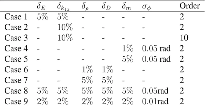
δE δk1x δρ δD δm σφ Order Case 1 5% 5% - - - - 2 Case 2 - 10% - - - - 2 Case 3 - 10% - - - - 10 Case 4 - - - - 1% 0.05 rad 2 Case 5 - - - - 5% 0.05 rad 2 Case 6 - - 1% 1% - - 2 Case 7 - - 5% 5% - - 2 Case 8 5% 5% 5% 5% 5% 0.05rad 2 Case 9 2% 2% 2% 2% 2% 0.01rad 2
Table 6: Sets of parameters
4.1
Deterministic case
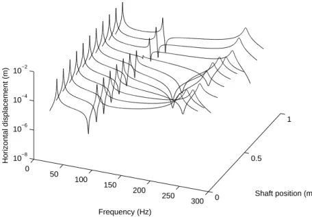
Before discussing the effects of uncertainties on the dynamic of the rotor system, a brief summary is given of the main dynamic characteristics of the deterministic rotor system. Considering the model parameters given in Table 1, Figure 3 shows the horizontal steady-state responses of the rotor for each of its transversal nodes.
It can be seen that the horizontal displacements indicate the presence of the first, second and third
forward critical speeds around 28.3 Hz, 97.2 Hz and 240 Hz, respectively. To facilitate
comprehen-sion, the first, second and third backward critical speeds do not appear on the unbalance responses due to the fact that the bearing stiffnesses are identical in the vertical and horizontal directions. Table 7 summarizes the values of the three first forward and backward critical speeds of the rotor system.
Critical speed Value (Hz)
1st backward 27.9 1st forward 28.3 2nd backward 61.8 2nd forward 97.2 3rd backward 128.1 3rd forward 240
Table 7: Critical speeds of the rotor system
4.2
Comparisons between the Polynomial Chaos Expansion approach and Monte
Carlo simulation
In this part of the paper, the results of the Monte Carlo simulation and those of the Polynomial Chaos Expansion method are compared in order to validate the efficiency of the second approach. Comparisons are given for the set of parameters defined by Case 1 in Table 6: to simulate the variation
0 50 100 150 200 250 300 0 0.5 1 10−8 10−6 10−4 10−2 Shaft position (m) Frequency (Hz) Horizontal displacement (m)
Figure 3: Frequency Response Functions for the determinism case
of mechanical properties, the Young modulus E of the shaft and the horizontal bearing stiffness k1x
on the left side of the rotor system are allowed to undergo5% variations (E ± δE and k1x± δk1x).
The Monte Carlo analysis is carried out to obtain a statistical sample of the random response. As explained previously, this method requires a large number of samples to provide a reference solution. In this study, to obtain convergence of the Monte Carlo method, 1000 samples were used. For this first case, the order of chaos equals 2. A convergence study, presented soon after, will justify the choice of this truncation.
Figures 4 and 5 show the mean and the variance of the Frequency Response Function (at the node 2 in the direction x) obtained by the two methods. The two methods yield quasi-identical results for
both quantities (a very low discrepancy can only be seen on peak around100 Hz) which validates the
PCE method.
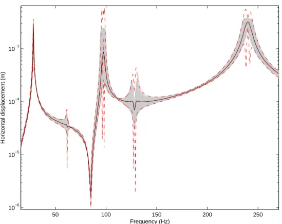
Figure 6 shows the results for both the Monte Carlo simulations and the PCE method. All the Frequency Response Functions samples obtained by using the Monte Carlo simulations can be seen at node 2 in the horizontal direction, with their mean value. We can see that the mean of the Frequency Responses Function and so the envelopes built from the Monte Carlo simulations and the Polynomial Chaos Expansion are very close one to the other. It should be noted that the same samples have been used for both direct Monte Carlo method and PCE approach. Moreover, for this example, if we compare the CPU time, it appears that PCE approach is eight times faster than the direct Monte Carlo approach.
The variations of the Young modulus E of the shaft and the horizontal bearing stiffness k1x can
be seen to cause small changes in the critical speeds. Moreover, increases (and decreases) of the maximum amplitudes when the rotor passes through the forward critical speeds are also indicated.
Finally, it can be seen that backward critical speeds (at 61.8 Hz and 128.1 Hz) can occur due to the
randomness of the bearing stiffness k1x which introduces dissymmetry in the rotor system.
A convergence study of the PCE with the order of chaos is performed through two choices of
orders : 2 and 10. Figures 7-8 and 9-10 present the results for cases 2 and 3 (10% of the variation
for the horizontal bearing stiffness k1x on the right side of the rotor system. See Table 6) for the
Frequency Response Functions at node 2 in the horizontal direction. As expected, the order of chaos improves modeling. However, the effect of this discrepancy between both expansions does not harm the quality of the model, especially when taking into account the increase of computation costs (which depends on the size of the problem as a function of the order of chaos) obtained subsequently. Even if the effect of damping is not on the scope of the study, it can be mentionned that decreasing the damping factor needs to increase the PCE order, especially close to the resonances. For more details, the reader is referred to the research of Dessombz [Dessombz (2000)].
50 100 150 200 250 10−5 10−4 10−3 Frequency (Hz) Horizontal displacement (m)
Figure 4: Mean of Frequency Response Functions (Case 1); Polynomial Chaos method (red dotted-dashed line); Monte Carlo Simulation (black line)
4.3
Effects of uncertainties in mechanical properties and external forces
In this part of the paper, the effects of uncertainties from stiffness properties of the rotor, geometric parameters of the disc and external forces are investigated. In the next paragraphs, only the mean
50 100 150 200 250 10−13 10−12 10−11 10−10 10−9 10−8 10−7 10−6 Frequency (Hz) Variance (m 2)
Figure 5: Variance of Frequency Response Functions (Case 1); Polynomial Chaos method (red dotted-dashed line); Monte Carlo Simulation (black line)
value and the envelope of the FRF are studied in order to highlight the results more clearly. It should be noted that in the following parts all the results are given at node 2 in direction x.
4.3.1 Excitation
The effects of uncertainties in the external forcing functions are now studied. Variations on the mass unbalance and the angular position are considered. Two cases are studied (cases 4 and 5): the first
and second cases deal with1% and 5% of uncertainties for both the mass unbalance and the angular
position (m± δmand φ± δφ).
Figures 11 and 12 illustrate the mean values (using the Monte Carlo simulation and the Polynomial Chaos method) and the envelope. In this particular case, the random quantities are only located at the
loading{Q}. Therefore, theoretically speaking, the mean of the response and the values of the critical
speed obtained by the Polynomial Chaos method must be identical to the reference mean response. In Figure 11, the mean of the Polynomial Chaos approach is close to the reference mean response: the error between these two results is only due to the truncated expansion of the loading expression defined in Equation (41).
It can then be seen that the variations of the maximum amplitudes due to uncertainties for all the critical speeds are not very great. The amplitudes of the first, second and third critical speeds increase
50 100 150 200 250 10−6 10−5 10−4 10−3 Frequency (Hz) Horizontal displacement (m)
Figure 6: Frequency Response Functions (Case 1); Mean of the FRF with Polynomial Chaos method (red dotted-dashed line); Lower and upper envelopes (red dashed line); Mean of the FRF with the Monte Carlo Simulation (black solid line); Monte Carlo samples (grey solid line)
from only2.814 × 10−3 m,2.803 × 10−3 m and3.76 × 10−3 m to2.954 × 10−3 m,3.534 × 10−3 m and 3.987 × 10⁻³ m respectively.
4.3.2 Uncertainties in disc properties
In this paragraph, variations for the properties of the disc located at the left side of the rotor system are considered. Two cases are investigated (cases 6 and 7): firstly, the density and the diameter of the
disc are allowed to undergo1% variations (ρ ± δρand D± δD). Secondly,5% variations on the same
set of parameters are introduced. As explained previously in Section 3.2, these random parameters affect the mass and gyroscopic matrices (see Equation (28)). The order of chaos has been chosen as equal to 2.
Figures 13 and 14 give the mean value of the Frequency Response Function and the envelope at node 2 in the horizontal direction. It appears that the mean values calculated by applying the Monte Carlo simulations and the Polynomial Chaos method are very similar. It should be noted that an order 2 gives accurate results in spite of the fact that the development given in Section 3.2 shows that an order 5 is needed to take all terms into account.
dras-50 100 150 200 250 10−5 10−4 10−3 Frequency (Hz) Horizontal displacement (m)
Figure 7: Study with chaos order2 : Mean of Frequency Response Functions (Case 2); Polynomial
Chaos method (red dotted-dashed line); Monte Carlo Simulation (black line)
tically affect the values of the critical speeds and the associated maximum amplitudes. Even if the maximum variations of amplitudes are located at the critical speed, the evolutions of the rotor response far from the critical speed are significant. When comparing Figures 6 and 14, it may be concluded that the effects of uncertainties on disc properties are greater than those on shaft properties of the rotor under study.
4.3.3 Uncertainties in both mechanical properties and external forces
In order to demonstrate the efficiency and accuracy of the Polynomial Chaos procedure described above, this last part of the paper treats the cases in which uncertain quantities come from all the parameters studied previously (i.e. stiffness properties of the rotor, geometric parameters of the disc and external forces).
Numerical simulations are given by considering the variations of mechanical properties of the shaft
(i.e. the Young modulus E and the horizontal bearing stiffness k1x), the properties of the disc (i.e.
the density ρ and the diameter D), and the excitation forces (i.e. the mass unbalance m and and the angular position φ), as indicated in Table 6 for cases 8 and 9. We recall that in this case the cost of calculation may be high since it is directly linked to the number of polynomials and consequently to the order of chaos and the number of random parameters. Figures 15-16 and 18-19 show the results
50 100 150 200 250 10−13 10−12 10−11 10−10 10−9 10−8 10−7 10−6 Frequency (Hz) Variance (m 2)
Figure 8: Study with chaos order2 : Variance of Frequency Response Functions (Case 2); Polynomial
Chaos method (red dotted-dashed line); Monte Carlo Simulation (black line)
for cases 8 and 9 through the mean and the variance obtained from the Polynomial Chaos and the Monte Carlo approaches. The results from both methods are in very good agreement for both the mean and for the variance. Figures 17 and 20 illustrate all the Frequency Response Function samples (at node 2 in the horizontal direction) obtained by using the Monte Carlo simulations, and the lower and upper envelopes built with the Polynomial Chaos method. It appears that increasing uncertainties affects the maximum amplitudes of the dynamic response and the value of the critical speeds. Then, as
explained previously in section 4.2, the dissymmetry due to the variations in the bearing stiffness k1x
leads to increases in the dynamic response of the rotor system around the backward critical speeds (at
61.8Hz and 128.1Hz). Finally, it can be seen that the Polynomial Chaos method may over-estimate
vibrational amplitude (see for example the dynamic response of the rotor around the third critical
speed, at240Hz). However, whatever the levels and different kinds of uncertainty (such as material,
geometrical and loading characteristics) presented here, the Polynomial Chaos method agrees very well with the Monte Carlo simulation, thereby demonstrating the robustness of the method.
50 100 150 200 250 10−5 10−4 10−3 Frequency (Hz) Horizontal displacement (m)
Figure 9: Study with chaos order10 : Mean of Frequency Response Functions (Case 3); Polynomial
Chaos method (red dotted-dashed line); Monte Carlo Simulation (black line)
5
Conclusion
This paper described a numerical procedure using the Chaos Polynomial approach to evaluate the stochastic response of a rotor system with uncertain mechanical parameters and uncertain external forces. It explained how this kind of problem can be solved with the Spectral Finite Element Method and how the random parameters can be modeled by random variables through a Karhunen-Loeve expansion. The results obtained by applying the Polynomial Chaos Expansion (PCE) procedure were compared with those evaluated by the Monte Carlo Simulation (MCS).
The stochastic response of the rotor system was proposed via the mean value and the variance of the random response and also represented graphically by an envelope. This envelope could be useful for designing rotor systems and predicting their lower and higher dynamic responses under uncertain parameters.
The efficiency and robustness of the Polynomial Chaos method were tested and validated through numerical simulations of the effects of uncertainties and orders of polynomial chaos.
50 100 150 200 250 10−13 10−12 10−11 10−10 10−9 10−8 10−7 10−6 Frequency (Hz) Variance (m 2)
Figure 10: Study with chaos order10 : Variance of Frequency Response Functions (Case 3);
Polyno-mial Chaos method (red dotted-dashed line); Monte Carlo Simulation (black line)
6
Acknowledgements
Jean-Jacques Sinou gratefully acknowledges the financial support of the French National Research Agency through the Young Researcher program ANR-07-JCJC-0059-01-CSD 2.
A
Model of the shaft
As illustrated in Figure 1, the nodal displacement of a beam element is defined by
δ = [v1w1θ1 ψ1 v2w2θ2 ψ2]T (46)
and for this element, the mass matrix [Me] = [Me
1] + [M e
2] (summation of the translational and
rotatory mass matrices), the stiffness matrix[Ke], the gyroscopic matrix [Ge] and the damping matrix
50 100 150 200 250 10−6 10−5 10−4 10−3 Frequency (Hz) Horizontal displacement (m)
Figure 11: FRFs with randomness on the loading (Case 4); Mean of the FRF with the Polynomial Chaos method (red dotted-dashed line); Lower and upper envelopes (red dashed line); Mean of the FRF with the Monte Carlo Simulation (black solid line)
[Me 1] = ρSl 420 156 0 0 −22l 54 0 0 13l 156 22l 0 0 54 −13l 0 4l2 0 0 13l −3l2 0 4l2 −13l 0 0 −3l2 156 0 0 22l 156 −22l 0 sym. −4l2 0 −4l2 (47)
50 100 150 200 250 10−6 10−5 10−4 10−3 Frequency (Hz) Horizontal displacement (m)
Figure 12: FRFs with randomness on the loading (Case 5); Mean of the FRF with the Polynomial Chaos method (red dotted-dashed line); Lower and upper envelopes (red dashed line); Mean of the FRF with the Monte Carlo Simulation (black solid line)
[Me 2] = ρI 30l 36 0 0 −3l −36 0 0 −3l 36 3l 0 0 −36 3l 0 4l2 0 0 −3l −l2 0 4l2 3l 0 0 −l2 36 0 0 3l 36 −3l 0 sym. 4l2 0 4l2 (48)
50 100 150 200 250 10−6 10−5 10−4 10−3 Frequency (Hz) Horizontal displacement (m)
Figure 13: FRFs with randomness on the disc parameters (Case 6); Mean of the FRF with the Poly-nomial Chaos method (red dotted-dashed line); Lower and upper envelopes (red dashed line); Mean of the FRF with the Monte Carlo Simulation (black solid line)
[Ke] = EI l3 12 0 0 6l −12 0 0 6l 12 −6l 0 0 −12 −6l 0 4l2 0 0 6l 2l2 0 4l2 −6l 0 0 2l2 12 0 0 −6l 12 6l 0 sym. 4l2 0 4l2 (49)
50 100 150 200 250 10−6 10−5 10−4 10−3 10−2 Frequency (Hz) Horizontal displacement (m)
Figure 14: FRFs with randomness on the disc parameters (Case 7); Mean of the FRF with the Poly-nomial Chaos method (red dotted-dashed line); Lower and upper envelopes (red dashed line); Mean of the FRF with the Monte Carlo Simulation (black solid line)
[Ge] = ρI 15l 0 −36 3l 0 0 36 3l 0 0 0 3l −36 0 0 3l 0 −4l2 3l 0 0 l2 0 0 3l −l2 0 0 −36 −3l 0 0 0 −3l skew− sym. 0 −4l2 0 (50)
in which ρ and E are the density and the Young modulus of the shaft. I is the second moment of the area about any axis perpendicular to the rotor axis. S is the area of the cross section.
50 100 150 200 250 10−5 10−4 10−3 Frequency (Hz) Horizontal displacement (m)
Figure 15: Mean of Frequency Response Functions (Case 8); Polynomial Chaos method (red dotted-dashed line); Monte Carlo Simulation (black line)
B
Mass and gyroscopic matrices components
md(τ ) = 1 4ρπh((D 2 − d2 ) + 2δDD 2 ξ3+ δρ(D 2 − d2 )ξ4+ D 2 δ2 Dξ 2 3 + 2δDδρD 2 ξ3ξ4+ δρδ 2 DD 2 ξ2 3ξ4) (51) = 4 X j=0 1 X i=0 mdijξ3jξ i 4 (52) Ip(τ ) = 1 32ρπh((D 4 − d4 ) + 4δDD 4 ξ3+ δρ(D 4 − d4 )ξ4+ 6D 4 δ2Dξ32+ 4δDδρD 4 ξ3ξ4+ 4δ 3 DD 4 ξ33 (53) + 6δρδ 2 DD 4 ξ23ξ4+ δ 4 DD 4 ξ34+ 4δ 3 DδρD 4 ξ33ξ4+ δρδ 4 DD 4 ξ34ξ4) = 4 X j=0 1 X i=0 Ipijξ3jξ i 4 (54)
50 100 150 200 250 10−12 10−11 10−10 10−9 10−8 10−7 10−6 Frequency (Hz) Variance (m 2)
Figure 16: Variance of Frequency Response Functions (Case 8); Polynomial Chaos method (red dotted-dashed line); Monte Carlo Simulation (black line)
Id(τ ) = 1 64ρπh((D 4 − d4 ) + 4δDD 4 ξ3+ δρ(D 4 − d4 )ξ4+ 6D 4 δD2ξ32+ 4δDδρD 4 ξ3ξ4+ 4δ 3 DD 4 ξ33 (55) + 6δρδ 2 DD 4 ξ32ξ4+ δ 4 DD 4 ξ34+ 4δ 3 DδρD 4 ξ33ξ4+ δρδ 4 DD 4 ξ34ξ4) + 1 48ρπh 3 ((D2− d2 ) + 2δDD 2 ξ3+ δρ(D 2 − d2 )ξ4+ D 2 δD2ξ32+ 2δDδρD 2 ξ3ξ4+ δρδ 2 DD 2 ξ32ξ4) = 4 X j=0 1 X i=0 Idijξ3jξ i 4 (56)
50 100 150 200 250 10−7 10−6 10−5 10−4 10−3 10−2 Frequency (Hz) Horizontal displacement (m)
Figure 17: Frequency Response Functions (Case 8); Mean of the FRF with the Polynomial Chaos method (red dotted-dashed line); Lower and upper envelopes (red dashed line); Mean of the FRF with the Monte Carlo Simulation (black solid line); Monte Carlo samples (grey solid line)
References
Benaroya, H., Rehak, M., (1988). Finite element methods in probabilistic structural analysis: A selective review. Applied Mechanics Reviews 41(5), 201–213.
Childs, D., (1993). Turbomachinery Rotordynamics: Phenomena, Modeling, and Analysis. Wiley Interscience.
Dessombz, O., (2000). Analyse dynamique de structures comportant des paramètres incertains. PhD Thesis, Ecole Centrale de Lyon.
Erich, F., (1992). Handbook of Rotordynamics. McGraw-Hill.
Friswell, M., Mottershead, J., (1995). Finite Element Model Updating in Structural Dynamics. Kluver Academic, Dordrecht.
Ghanem, R., (1999). Stochastic finite elements with multiple random non-gaussian properties. Journal of Engineering Mechanics 125, 26–40.
50 100 150 200 250 10−5 10−4 10−3 Frequency (Hz) Horizontal displacement (m)
Figure 18: Mean of Frequency Response Functions (Case 9); Polynomial Chaos method (red dotted-dashed line); Monte Carlo Simulation (black line)
Ghanem, R., Spanos, P., (1991). Stochastic Finite Elements: A Spectral Approach. Springer-Verlag.
Lalanne, M., Ferraris, G., (1990). Rotordynamics-Prediction in Engineering. John Wiley & Sons,
New York.
Nayfeh, A., (1973). Perturbation Methods. John Wiley and Sons, London.
Wiener, N., (1938). The homogeneous chaos. American Journal of Mathematics 60, 897–936. Yamamoto, T., Ishida, Y., (2001). Linear and Nonlinear Rotordynamics: A Modern Treatment with
Applications. Wiley and Sons.
Yamazaki, F., Shinozuka, M., Dasgupta, G., (1988). Neumann expansion for stochastic finite element analysis. Journal of Engineering Mechanics, ASCE 114(8), 1335–1354.
50 100 150 200 250 10−13 10−12 10−11 10−10 10−9 10−8 10−7 10−6 Frequency (Hz) Variance (m 2)
Figure 19: Variance of Frequency Response Functions (Case 9); Polynomial Chaos method (red dotted-dashed line); Monte Carlo Simulation (black line)
50 100 150 200 250 10−6 10−5 10−4 10−3 10−2 Frequency (Hz) Horizontal displacement (m)
Figure 20: Frequency Response Functions (Case 9); Mean of the FRF with the Polynomial Chaos method (red dotted-dashed line); Lower and upper envelopes (red dashed line); Mean of the FRF with the Monte Carlo Simulation (black solid line); Monte Carlo samples (grey solid line)