HAL Id: hal-00773522
https://hal.archives-ouvertes.fr/hal-00773522
Submitted on 14 Jan 2013
HAL is a multi-disciplinary open access archive for the deposit and dissemination of sci-entific research documents, whether they are pub-lished or not. The documents may come from teaching and research institutions in France or abroad, or from public or private research centers.
L’archive ouverte pluridisciplinaire HAL, est destinée au dépôt et à la diffusion de documents scientifiques de niveau recherche, publiés ou non, émanant des établissements d’enseignement et de recherche français ou étrangers, des laboratoires publics ou privés.
levels in continental waters. Toward the determination
of threshold values
J.P. Besse, Marina Coquery, C. Lopes, Arnaud Chaumot, H. Budzinski, P.
Labadie, O. Geffard
To cite this version:
J.P. Besse, Marina Coquery, C. Lopes, Arnaud Chaumot, H. Budzinski, et al.. Caged Gammarus fossarum (crustacea) as a robust tool for the characterization of bioavailable contamination levels in continental waters. Toward the determination of threshold values. Water Research, IWA Publishing, 2013, 47 (2), p. 650 - p. 660. �10.1016/j.watres.2012.10.024�. �hal-00773522�
Caged Gammarus fossarum (crustacea) as a robust tool for the
characterization of bioavailable contamination levels in continental waters.
Toward the determination of threshold values
Authors
BESSE Jean-Philippe (First author) a
COQUERY Marina a LOPES Christelle a CHAUMOT Arnaud a BUDZINSKI Hélène b LABADIE Pierre b GEFFARD Olivier a* mail: [email protected] phone number : (+33) 4 72 20 89 05
a: Irstea, UR MALY (Freshwater Systems, Ecology and Pollution), 5 rue de la Doua, CS70077, 69626 VILLEURBANNE Cedex, France
Phone : (+33) 4 72 20 87 85 Fax : (+33) 4 78 47 78 75
b: Université Bordeaux 1, Environnements et Paléoenvironnements Océaniques et
Continentaux (EPOC) - UMR 5805 CNRS, Laboratoire de Physico- et Toxico-Chimie de l'environnement (LPTC), 351 cours de la Libération, 33405 Talence, France.
Abstract
We investigated the suitability of an active biomonitoring approach, using the ecologically relevant species Gammarus fossarum, to assess trends of bioavailable contamination in continental waters. Gammarids were translocated into cages at 27 sites, in the Rhône-Alpes region (France) during early autumn 2009. Study sites were chosen to represent different physico-chemical characteristics and various anthropic pressures. Biotic factors such as sex, weight and food availability were controlled in order to provide robust and comparable results. After one week of exposure, concentrations of 11 metals/metalloids (Cd, Pb, Hg, Ni, Zn, Cr, Co, Cu, As, Se and Ag) and 38 hydrophobic organic substances including polycyclic aromatic hydrocarbons (PAHs), polychlorobiphenyles (PCBs), pentabromodiphenylethers (PBDEs) and organochlorine pesticides, were measured in gammarids. All metals except Ag, and 33 organic substances among 38 were quantified in G. fossarum, showing that this species is relevant for chemical biomonitoring. The control of biotic factors allowed a robust and direct inter-site comparison of the bioavailable contamination levels. Overall, our results show the interest and robustness of the proposed methodological approach for assessing trends of bioavailable contamination, notably for metals and hydrophobic organic contaminants, in continental waters.
Furthermore, we built threshold values of bioavailable contamination in gammarids, above which measured concentrations are expected to reveal a bioavailable contamination at the sampling site. Two ways to define such values were investigated, a statistical approach and a model fit. Threshold values were determined for almost all the substances investigated in this study and similar values were generally derived from the two approaches. Then, levels of contaminants measured in G. fossarum at the 27 study were compared to the threshold values obtained using the model fit. These threshold values could serve as a basis for further
implementation of quality grids to rank sites according to the extent of the bioavailable contamination, with regard to the applied methodology.
Keywords
Active biomonitoring; threshold values; bioaccumulation; gammarids; freshwaters, priority substances
1. Introduction
The use of biota to monitor levels and trends of chemical contamination in water (i.e.,
chemical biomonitoring) was suggested in the mid-1970s for costal waters (Goldberg, 1975), and has been thereafter used in several monitoring programmes in costal and continental waters (Besse et al., 2012). As an integrative matrix, biota enables reliable measures for trace metals and hydrophobic contaminants, as the higher levels retained by the organisms can be more easily measured. Moreover, biota reflects the bioaccumulative and bioavailable fraction of contaminants in receiving waters, which are of direct ecotoxicological relevance. Finally, biota enables time-integrated measures over the exposure period, so it can be used to establish spatial and temporal trends of a bioavailable contamination (EC, 2010; Andral et al., 2004; Rainbow 1995).
Currently, two different strategies of chemical biomonitoring can be adopted: passive and active biomonitoring. Passive approaches rely on indigenous organisms (Sudaryanto et al. 2002; Goldberg 1975), while active ones rely on transplanted (or caged) individuals from a reference site (Benedicto et al., 2011; Andral et al., 2004). Even though passive approaches have proved useful for monitoring contamination trends for metals and several organic contaminants, they are recognized as suffering from two major drawbacks: i) they depend on the effective presence of the native organism at the sampled sites; and, ii) several factors (e.g., variability in the exposure time, age and size of sampled organisms) may hinder accurate interpretation of the results (Besse et al., 2012). Active approaches, based on transplanted organisms, have been developed more recently with the aim of resolving these limitations. Indeed, active approaches can be applied even if study sites are devoid of native organisms, they allow limiting biological variability as organisms are collected from the same population, and the exposure time can be controlled (Bourgeaut et al., 2010; Bervoets et al. 2005; Andral
et al. 2004; Mersch et al. 1996). If some active biomonitoring programs have been
implemented in the marine environment (Benedicto et al., 2011; Andral et al., 2004), no such approaches have been undertaken at a large scale to monitor contamination in continental waters.
Therefore, the first objective of this study was to investigate the relevance and robustness of an active biomonitoring strategy, using the amphipod Gammarus fossarum to monitor trends of bioavailable contamination for trace metals and hydrophobic contaminants in continental waters.
The amphipod species Gammarus fossarum was selected as the test organism as gammarids are widespread and common in rivers and streams of Western Europe, where they are often present at high density. They are ecologically relevant as they represent an important reserve of food for macroinvertebrate, fish, bird and amphibian species and also play a major part in leaf litter breakdown processes (Macneil et al. 1997; Welton 1979). Moreover, G. fossarum is easy to identify down to the species level and its physiology is quite well known (Coulaud et al., 2011; Lacaze et al., 2011; Dedourge-Geffard et al., 2009). Finally, a well defined caging protocol is available for this species, allowing to control biological characteristics such as size, sex, supply of food; and it has been widely used for several studies in ecotoxicology (Coulaud et al., 2011; Lacaze et al., 2011; Dedourge-Geffard et al., 2009). As organisms are caged and as their only source of food is the one provided at the beginning of the experiment, concentrations measured in gammarids are to be regarded as mainly proceeding from the dissolved phase and not from the trophic route.
The second objective of this study was to benefit from such a caging approach to determine threshold values of bioavailable contamination, assuming that measured concentrations above the threshold values could be considered as representative of a bioavailable contamination at
the sampling site, whereas values under the threshold values would only reflect the background level of contamination.
Such threshold are expected to i) allow the identification of problematic contaminants on the basis of the bioavailable fraction, and ii) serve as a basis for any further implementation of quality grids that would allow to rank sites according to the extent of the bioavailable
contamination. For instance, in continental waters, threshold values have been determined in aquatic bryophytes (by passive monitoring) to improve the interpretation of results and to build quality grids of metal contamination (AE, 1998). Furthermore, with regard to the marine environment, the OSPAR Commission has built some statistical tools that enable testing whether the mean measured concentrations (in sediment or biota) can be considered to be near background concentrations or is representative of an effective contamination of the sampling site (ICES, 2004).
To fulfil the two objectives of this study – investigating the relevance and robustness of the caging strategy, and determining threshold values of bioavailable contamination – individuals of Gammarus fossarum were caged for 7 days at 27 sites of rivers of the Rhône-Alpes region (France) and 49 contaminants (11 metals and 38 hydrophobic organic substances) were monitored. Sites were chosen for their differences in watershed size, physico-chemical characteristics and anthropic pressures.
2. Materials and methods
2.1. Sampling and handling of tests organisms
Gammarids were collected at “La Tour du Pin”, a known unpolluted upstream part of the Bourbre River (France). This station displayed good water quality according to RNB data
records (French Watershed Biomonitoring Network), and a high density of gammarids was found. Sexually mature G. fossarum were collected using a hand-held net. Gammarids were sieved (2-2.5 mm) to separate juveniles and adults, and were stored in plastic bottles
containing ambient freshwater, then quickly brought to the laboratory. The organisms were kept during a 15 days acclimatisation period in 30 L tanks under constant aeration. A 10/14 h light/dark photoperiod was maintained and the temperature was kept at 12 (±1) °C. They were continuously supplied with groundwater mixed with osmosis water at two different constant water hardness: 112 or 223 mg L−1 of CaCO3, depending on the hardness level of the
subsequent studied site. Organisms were fed ad libitum with alder leaves (Alnus glutinosa) collected in a pristine site and previously conditioned for at least 6 (±1) days in groundwater. Twice a week freeze-dried Tubifex sp. worms were added as a dietary supplement.
2.2. Caging procedure
The caging procedure applied here is derived from the one formerly used for in situ toxicity assessment and for the development of biomarkers (Coulaud et al., 2011; Lacaze et al., 2011; Dedourge-Geffard et al., 2009).
Gammarids were caged in polypropylene cylinders (length, 10 cm; diameter, 5.5 cm) capped at their ends with pieces of net (mesh: 1 mm) to guarantee free water flow. Twenty-four hours before initiating the experiment, pools of 25 individual G. fossarum were placed in the
cylinders. Eight experimental cylinders were placed into a rigid plastic container to protect them. The containers were subsequently positioned parallel to the direction of water flow and secured to the streambed using natural rocks. To limit the influence of body length, growth and sex on contaminants accumulation, only mature and same age-ranked gammarids were exposed: male G. fossarum with an average body length of 9 ± 1 mm and an average weight
ranging from 4 to 6 mg (dry weight) were selected. To avoid the influence of starvation on survival rate and contaminants uptake, 20 alder leaf (A. glutinosa, same as in laboratory) discs (20 mm in diameter) were supplied into each cage.
After 7 days of exposure, gammarids were collected, counted (for survival rate assessment), dried, weighted, frozen in liquid nitrogen and stored at −80 °C until chemical analyses. Temperature probes were fixed to one cage at each site, so that measurements could be carried out twice a day throughout the experiment. The measure of hardness was also carried out at the laboratory from grab samples collected at the beginning and at the end of the exposure.
2.3. Study sites
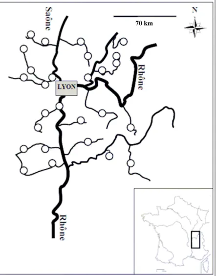
The experiment was conducted in September 2009. Twenty-seven sites were selected in the Rhône-Alpes region aiming at covering a large range of geographical locations
(approximately 20 000 km2), various types of hydrological systems and a large range of physico-chemical characteristics (Figure 1, Table S1 and S2).
For our study, the sites were also selected seeking to cover diverse anthropogenic pressures (industrial, urban and agricultural activities). Within these 27 sites, 12 sites (1-12) were chosen as non- impacted sites among the national reference network (Water Framework Directive- WFD - implementation) in collaboration with the regional public water agency (http://sierm.eaurmc.fr/eaux-superficielles). According to expert judgement based on data on land use, chemical monitoring (macropollutans and some micropollutants), and ecological diagnosis, these sites were considered to be devoid of (or to showing limited) anthropic pressure. The 15 other sites (13-27) were chosen as impacted sites among the national control network (WFD implementation) by the regional water agency
(http://sierm.eaurmc.fr/eaux-superficielles). According to the expert classification based on data on land use, degraded
water chemical quality (macropollutants and some micropollutants) and/or poor faunistic indices, these sites were considered impacted by anthropic activities. Detailed physico-chemical characteristics for all studied sites (i.e., surface water temperature, dissolved oxygen, pH and hardness), and pressure types for the 15 anthropically impacted sites are presented in supplementary data, Tables S1 and S2. For data treatment, and notably for the determination of threshold values, study sites were used together, not taking into account their
a priori contamination level.
2.4. Choice of contaminants and chemical analysis
A total of 49 contaminants were investigated in this study, including 22 chosen with reference to the list of WFD priority substances (EC, 2008). The list included 11 metals or metalloids: Cd, Pb, Hg, Ni (WFD priority substances; EC, 2008) and Ag, As, Co, Cr, Cu, Se and Zn. Also, 38 hydrophobic organic substances (log Kow > 3) were investigated including
chlorinated pesticides (among which 8 WFD priority substances): lindane, hexachlorobenzene (HCB), dichlorodiphenyltrichloroethane (DDT) isomers and metabolites (2,4' DDE; 4,4' DDE + dieldrin; 2, 4'-DDD; 4, 4'-DDD; 2, 4'-DDT; 4,4'-DDT); heptachlor and heptachlor epoxide; 7 indicator PCBs: CB n° 28, 52, 101, 118, 138, 153 and 180; 4 congeners of PBDEs (among which 3 WFD priority substances): BDE n° 47, 99, 119 and 153; and 16 PAHs (among which 7 WFD priority substances): naphthalene, anthracene, fluoranthene, benzo(a)pyrene (BaP), benzo(b,k,j)fluoranthenes, indeno(1,2,3-cd)pyrene, benzo(g,h,i)perylene (BP); and
acenaphthylene, acenaphtene, fluorene, phenanthrene, pyrene, benzo(a)anthracene, benzo(e)pyrene, triphene +chrysene, perylene and dibenzo(a)anthracene +
2.4.1. Metal analysis
Individuals of G. fossarum were pooled (5 organisms per sample) to obtain an average mass of 30 mg dry weight (about 150 mg wet weight). Three replicates of each pooled sample were subjected to analysis. All chemical analyses were conducted at the Irstea of Lyon. Metals (Cd, Pb, Hg, Ni, Ag, As, Co, Cr, Cu, Se and Zn) were analysed by inductively coupled plasma mass spectrometry (ICP-MS, Thermo X7 series II), after mineralization with nitric acid in a microwave oven. For Hg, samples were analyzed by automated atomic absorption
spectrometry (MILESTONE, Direct Mercury Analyser 80).
Blank tests were carried out systematically to detect any possible contamination along the analytical chain. The following certified reference materials (CRM) were used for quality control for metals: National Research Council Canada (NRCC) TORT-2, lobster
hepatopancreas, and International Atomic Energy Agency IAEA-407, fish. For Hg, National Institute of Standards and Technology Standard Reference Material (NIST) SRM-2976 and Institute for Reference Materials and Measurements (IRMM) CRM 278 R, mussel tissue, were used. The limits of quantification (LQ), determined according to NF XPT 90-210 (AFNOR, 1999), are detailed in Table 1. The CRM results were generally well within certified values. Relative standard deviations of triplicate pooled sample analyses (including sampling and analytical variability) were generally below 20%.
2.4.2. Organic substances analysis
All chemical analysis were carried out at the Centre de Développement et de Transfert Analytique (CDTA, Bordeaux). Individuals of G. fossarum were pooled (75 organisms per
sample) to obtain an average mass of 2300 mg wet weight (i.e., approximately 400 mg dry weight). Extraction and quantification methods for PAHs, PCBs and organochlorine
pesticides are described elsewhere in detail (Cailleaud et al., 2007; Thompson and Budzinski, 2000). Briefly, contaminants accumulated in G. fossarum were extracted using
dichloromethane by microwave-assisted extraction (Maxidigest 350 VWR, Fontenay sous Bois, France). The organic extracts were then purified. Concentrations of PCBs and organochlorine pesticides on the one hand and of PAHs on the other hand were measured, respectively, using a gas chromatography (GC)/electron capture detector (Hewlett-Packard 5890A series IIGC, Avondale, MA, USA) equipped with a 63Ni electron-capture detector) and GC/mass spectrometry (Hewlett-Packard model series 6890A GC and an Agilent Networks 5973 mass selective detector, Agilent Technologies, Santa Clara, CA, USA). The LQ are detailed in Table 2.
Procedural blanks (glass material and solvents) were regularly performed. The effectiveness of the different analytical procedures was evaluated by analyzing National Institute of
Standards and Technology Standard Reference Material (NIST) SRM-2978, mussel tissue, for PCBs and PAHs.
2.5. Determination of threshold values of contamination
To determine threshold values of bioavailable contamination, G. fossarum concentrations for each contaminant were first sorted by increasing value. From such a representation, we subsequently determined the threshold value from which the concentration measured in G.
fossarum could be considered as significant. For that, two different approaches were
investigated: the first one based on a statistical approach (normality assumption), and the second one based on a model fit (bacterial growth model).
2.5.1. Statistical approach
The first method was based on the assumption that contamination levels in organisms would be normally distributed only at sites devoid of any bioavailable anthropogenic and/or
geochemical background contamination. For each substance and values higher than the LQ, we tested if the overall data set followed a Gaussian distribution (using Shapiro test). If not, the most contaminated site was removed from the data set and the normality tested again. Such an iterative process was conducted until a data set normally distributed was obtained. The threshold value for each substance was determined from the respective Gaussian
distribution obtained by the 95th percentile, with a risk of false negative set at 5% (Figure 2). The iterative procedure was implemented using the R statistical computing program (R Development Core Team, 2007).
2.5.2. Model fit
The second method was based on the observation that contamination levels in gammarids followed the same overall pattern as bacterial growth kinetic: with a latent period
(corresponding here to the background level of contamination in organisms), and an
exponential phase (corresponding to the significative phase of accumulation). Therefore, the distribution of contamination levels, sorted by increasing values, was fitted using a bacterial growth model, the Barranyi’s model, following Equation 1 (Baranyi et al., 1993).
( )
( )
(
)
( )
( )
(
(
)
()
) + + − + + − + = − 0 max 10 * * exp * exp 1 * exp * exp 1 log log log10 10 max 10 C C lag t lag t C t C µ µ µ µ Equation 1where C(t) is the concentration at site t; Cmax is the maximal concentration; µ is the
accumulation rate; lag is the point from which the exponential phase of accumulation begins; and C0 is the minimal concentration.
The “lag” allowed separating the background level of contamination from the significant phase of accumulation, and was used as the break point from which the threshold value of contamination was estimated (Figure 3). The calculation was performed using the R statistical computing program. The parameters of the Baranyi’s model fitted to the data were estimated by nonlinear regression using the “nlstools” package
(http://cran.r-project.org/web/packages/nlstools/nlstools.pdf).
3. Results
3.1. Quantification of contaminants in Gammarus fossarum
After the 7 days of exposure, gammarids survival rate remained high, with a mean survival rate higher than 75% at all but one site (site 27, Supplementary data, Figure S1).
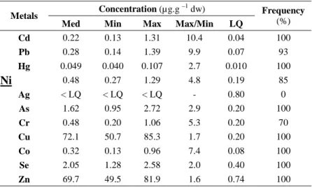
Contamination levels in G. fossarum are presented in Table 1 for metals (or metalloids) and in Table 2 for organic substances. Considering metals/metalloids, nearly all measured values were higher than the LQ. Cd, Hg, As, Cu, Co, Se and Zn were always quantified, while Pb, Ni, and Cr were quantified at all but 2, 4, and 8 sites, respectively. Only Ag was not quantified at all among the 27 sites. For organic substances, most of them were also quantified in caged G. fossarum, with only 5 substances never detected: heptachlor, heptachlor epoxide, 2,4’-DDD and BDE congeners n° 119 and 153 (Table 2). Some DDT isomers (namely 4,4’-DDE + dieldrin; 4,4’-DDT and 2,4’-DDT), BDE congeners (47 and
153), some PAHs (naphthalene, acenaphtene, pyrene, benzo(a)anthracene, and triphene + chrysene), and all PCB congeners were always quantified.
To estimate the capacity of accumulation of G. fossarum with regard to the investigated contaminants, empirical factors (ratio maximal concentration/minimal) were assessed. Except for Zn and Cu, all ratio were higher than 2, with values up to 100 for organic contaminants (phenanthrene, 2,4’-DDT).
3.2. Threshold values of contamination
Threshold values determined for contaminants investigated here are displayed in Table 3. The statistical approach provided a threshold value for all studied substances with concentrations higher than the LQ (i.e., 43 substances), whereas the model fit could not provide threshold values for 8 contaminants: 5 metals (As, Cr, Cu, As, Se and Zn), and 3 organic substances (naphthalene, DaA-DaC, and BDE 47).
For a single substance, threshold values calculated using the two approaches were very close to each other (Table 3): the maximum interval observed between two values was of 0.1 µg.g-1 for metals (observed for Ni) and 3.1 ng.g-1 for organics (observed for phenanthrene).
4. Discussion
4.1. Suitability G. fossarum as a biomonitor of chemical contamination in continental waters.
Contrary to other freshwater invertebrates, such as the invasive bivalve Dreissena
polymorpha, gammarids have not been much used to monitor chemical contamination in
1996) and active biomonitoring (Lacaze et al., 2011; Dedourge-Geffard et al., 2009; Khan et al., 2011) are available. Mean and median values reported in these latter studies (for Cd, Ni, Pb, As, Co, Cr, and Zn) for rivers are in the same range as values observed here. For organic substances investigated here, and for continental waters, no data from active biomonitoring were found in the scientific literature and only very few data from passive biomonitoring are available (Blais et al., 2003). Heptachlor was measured in G. lacustris, at around 0.1 ng.g-1 wet weight (about 0.5 ng.g-1 dry weight, assuming 80% moisture). These results suggest that, even if uptake rates may differ between the two species, the absence of quantification of this substance in our study was not linked to a low accumulation in G. fossarum, but rather to an absence of contamination of the study sites by this contaminant. Our results show that almost all investigated substances accumulated well and could be quantified in G. fossarum, on a relatively short exposure period (Tables 1 and 2). Moreover, the high Max/Min ratios measured for most of the organic contaminants studied suggest that G. fossarum is a good accumulator and a suitable species for monitoring chemical contamination in continental waters. Indeed, as stated by Rainbow (2002), the fact that the sampled organism is a strong accumulator increases the power of resolution between sites. Nonetheless, the suitability of G.
fossarum for chemical monitoring is limited in the specific case of Cu: indeed, gammarids are
known to be poor indicators for this metal, as Cu is involved in haemocyanin synthesis, and is therefore highly regulated in all gammarid species (Dedourge-Geffard et al., 2009; Taylor and Anstiss, 1999).
Finally, considering the analytical methodologies used in this study, only a limited amount of tissue matrix was necessary to quantify the contaminants investigated here: about 5 organisms (approximatively 150 mg wet weight) for all metals but Hg, 5 organisms for Hg, and 75 organisms (approximatively 2300 mg wet weight) for all organic substances.
4.2. Robustness of the active methodology for chemical monitoring
During this study, we focused on showing the robustness of the methodology and the comparability of the results. The methodology proposed here (organisms of same sex, same weight and supplemented with food) allowed obviating any influence of biotic factors on tissue levels of contaminants. At the end of the exposure, only minor variations of weight were observed (mean of 5.8 mg dry weight per organism, with a standard deviation of 0.7 mg). Selecting mature organisms with the same weight allowed avoiding any confounding effect of this parameter, which is considered by several authors as one of the main factor that can influence tissue levels of contaminants (Geffard et al., 2007; Mubiana et al., 2006; Andral et al., 2004; Boyden, 1974).
Supplementing gammarids with food ensures an optimal survival rates and prevents from any growth variation linked with food availability, which is a clear advantage over bivalves. In fact, the accumulation of contaminants depends on the organism growth (Andral et al., 2004). Hence, as shown for bivalves, caged organisms exposed in sites of different trophic potential may exhibit different growth rates, which prevent a direct comparison of tissue
concentrations. In such cases, there is a need to correct raw data to account for various growth rates (Bourgeault et al., 2010; Andral et al. 2004; Mersch et al., 1996).
Contrary to biotic factors, the influence of abiotic factors cannot be controlled in our methodology. Such factors can be suspected to perturb the physiology of organisms and therefore to influence levels of contamination in G. fossarum. As an example, the role of temperature on bivalves’ physiology and on bioaccumulation is commonly emphasised (Minier et al., 2006; Gossiaux et al., 1996). Considering the conditions of this study, no influence of temperaturewas observed. This could be linked to the fact that the observed temperatures during the exposure (minimum of 8.6°C, maximum of 19.7°C; Supplementary
data, Table S3) were all within the tolerance range for G. fossarum, which is estimated to be from 0°C to 25°C, with an optimum temperature of 12°C (Wijnhoven et al., 2003).
Furthermore, for gammarids, results of a laboratory experiment indicated that temperature has only a weak effect on metals accumulation (Pellet et al., 2009). Moreover, results of a field study on the accumulation of organic pesticides and PCBs in gammarids suggested that temperature has a negligible influence on tissue levels of contaminants when compared to the growth rate of organisms (Blais et al., 2003).
Although the impact of hardness on metal speciation and bioavailability is well known (Lebrun et al., 2011; Peters et al., 2011; Heijerick et al., 2003; Wright & Frain, 1981), its influence on the physiology of organisms, in particular on the density of sites of action of metal transporters, and subsequently on the accumulation of metals in organisms, has been poorly studied to date. Ma et al. (1999) showed that Cu uptake in Ceriodaphnia dubia did not change when organisms were grown in water with high or low Ca2+ concentration levels. In contrast, Pellet et al. (2009) showed that Cd influx in G. pulex decreased as Ca2+ concentrations increased due to the decrease of Cd bioavailability resulting from the competition between Ca2+ and Cd. In the study sites, hardness ranged from 15 to 290 mg.L-1 of CaCO3 ((Supplementary data, Table S1, S2); no influence of hardness on contamination
levels of organisms was observed. To suppress the effect of hardness, G. fossarum was acclimated to appropriate level of hardness (see section 2.1.) prior to the biomonitoring. Thus, the effects of hardness on the physiology of gammarids are expected to be negligible.
4.3. Threshold values of bioavailable contamination
This is the first study dealing with the determination of threshold values of bioavailable contamination in biota for metals and hydrophobic substances. Consequently, it is only possible to propose preliminary statements on the validity of the calculated threshold values. As a first approach, threshold values were considered to be valid for a given substance when i) a threshold value could be calculated via the two different approaches and ii) the values given by the two approaches were close to each other. To verify the second statement, we compared the difference between the two values to the maximum concentration measured in gammarids, using Equation 2 (”Reliability ratio”). We consider that the lower the ratio, the more reliable the threshold value.
Reliability ratio = − ×100 ion concentrat measured Maximum Threshold Threshold stat fit
Equation 2
Results are displayed in Table 3. For the 35 contaminants for which the two methodologies provided a threshold value, reliability ratios were very low (<0.1) for all but 5 contaminants, and the highest ratio (0.3) was observed for Hg and BDE 99. Therefore, we consider these threshold values as valid.
4.3.2. Unvalid threshold values
Threshold value for Cu, obtained using the statistical approach only, was expected to be unvalid. In fact, as discussed in section 4.1., gammarids are poor indicators for this metal as they are able to regulate it. Thus, contrary to other contaminants, distribution of the measured concentrations of Cu showed a specific profile (i.e., not gaussian, or without an exponential phase; Supplementary data, Figure S2).
For 7 other contaminants (As, Cr, Se, Zn, naphthalene, DaA-DaC and BDE 47), only the statistical approach provided a threshold value (Table 3, Figure S2 of supplementary data) so
their validity is questionnable. Unvalidity may stem from the overall absence of
contamination, or conversely, from the presence of a significant bioavailable contamination at all study sites. In fact, for these 7 contaminants, the whole datasets followed a normal
distribution. Hence, if we assume that contamination levels in organisms are normally distributed only at sites devoid of any anthropogenic pressure, such results suggest that measured concentrations at the 27 sites were only representative of the “background” impregnation. This is also in agreement with the fact that no threshold value could be
determined using the model fit (i.e., measured concentrations only representative of the latent phase of bioaccumulation).
Such an hypothesis could be verified in the case of Zn. We included additional
bioaccumulation data obtained from a previous study on metal impacted sites, based on the same gammarus species and a similar exposure protocol, and showing concentrations in gammarids up to 237 µg.g-1 dw (Lacaze et al., 2011). We obtained threshold values using both calculation methods, slightly above maximum concentrations measured in the present study. Such results underline the need to obtain bioaccumulation data representative of contaminated areas to determine valid thresholds.
Overall, our results support the relevance of the two methodologies (i.e., statistical approach or model fit) to determine threshold values of bioavailable contamination in caged G.
fossarum.
4.3.3. Application of the threshold values
As a preliminary application of our defined threshold values, we classified the study sites according to valid thresholds obtained with the model fit (Table 4).
For organic contaminants, this classification showed that 15 sites (#1 to 11, 13, 16, 18 and 26) displayed less than 5 substances exceeding thresholds. For these 15 sites - except sites 16, 18 and 26 - these results support the expertise of water agency (Supplementary data, Table S1 and S2), as these sites did not show a bioavailable contamination for most of the investigated substances. For sites 16, 18 and 26, observed discrepancies with the expertise of water agency may stem from one of the following reasons : i) conclusions obtained from experts did not take into account the physico-chemical parameters of study sites, whereas they play a key role in the bioavailability of pollutants, ii) contamination levels were determined in caged
organisms for a duration exposure of 1 week, and therefore, do not integrate contamination variability that may exist in aquatic systems, and iii) sites may be contaminated by other organic substances than the ones investigated here.
Conversely, 7 other sites (# 12, 14, 19, 22, 23, 24 and 27) had concentrations in gammarids higher than the threshold values for several organic substances and displayed distinguishable profiles of contamination. For instance, sites 12, 23, 24 and 27 showed a clear contamination of PAHs and PCBs, and site 19 displayed a specific contamination of pesticides and PCBs. Hence, these results show that threshold values are valuable tools to identify sites showing a bioavailable contamination, to identify problematic contaminants and to draw typologies of contamination. This is of value for river basin authorities for establishing strategic framework for the management of waterbodies.
For metals, the threshold classification showed that only 10 sites among the 27 did not display any concentration higher than the threshold values, while most of the sites showed a
contamination by Cd and Pb, and site 18 had a specific contamination profile with Hg, Ni and Co. With regard to the expert classification of the Water Agency, numerous discrepancies were observed. Indeed, sites 1 to 12 were expected to be devoid of any anthropic pressure (Section 2.3.). Such discrepancies may stem from the presence of i) an anthropogenic source
of contamination not pre-identified, or ii) a local geochemical background. Currently, available information is too scarce to draw any definitive conclusion, but we note that these sites are localized in the Western part of the Rhône-Alpes region, near the “Massif Central” mountain range, known to present elevated geochemical backgrounds for As, Cd and Pb (Cf. FOREGS Geochemical Baseline Mapping Programme; http://www.gsf.fi/publ/foregsatlas).
5. Conclusion
Results of this study showed that caged Gammarus fossarum is a robust and useful tool to monitor bioavailable contamination trends of metals and hydrophobic organic substances in continental waters. The two most important advantages of this methodology are i) that it can be applied even is the study site is devoid from native organisms and ii) that it provides results that enable a direct comparison of bioavailable contamination trends among different sites.
Moreover, using two simple calculation approaches, we were able to determine valid threshold values of bioavailable contamination in G. fossarum. These threshold values allowed discriminating background levels of contamination from any significant
bioaccumulation in gammarids, thus indicating a bioavailable contamination at the sampling site. Such threshold values could further serve as a basis for the implementation of a quality grid that would allow ranking sites according to the extent of the bioavailable contamination, and with regard to the applied methodology. To our knowledge, this was the first study to investigate the implementation of such threshold values in the context of active
biomonitoring.
Next step in our work will focus on the following objectives: investigating the
validating the threshold values by conducting additional studies at national scale in France, taking into account various river systems and different anthropic pressures. Such an effort is necessary to clearly establish if the defined threshold values are dependent or not of
hydrogeochemical characteristics and if they need some adjustment. Finally, investigating longer duration of exposure will allow assessing whether threshold values also depend on the exposure time.
Acknowledgments
Authors thank ONEMA (the French National Agency for Water and Aquatic Ecosystems) for its financial support. Authors also thank technical staff of Irstea for their assistance in the field experiments and for analyses of trace elements.
References
AE (1998) Les bryophytes aquatiques comme outil de surveillance de la contamination des eaux courantes par les micropolluants métalliques. Concept, méthodologie et interprétation des données. Etude inter-agences n° 55.
AFNOR, Norme NF XPT 90-210, Protocole d’évaluation d’une méthode alternative d’analyse physico-chimique par rapport à une méthode de référence, 1999, 58 pp.
(www.boutique.afnor.org/).
Amyot, M., Pinel-Alloul, B., Campbell, P.G.C., Désy, J.C. (1996) Total metal burdens in the freshwater amphipod Gammarus fasciatus: Contribution of various body parts and influence of gut contents. Freshwater Biology 35(2), 363-373.
Andral, B., Stanisiere, J.Y., Sauzade, D., Damier, E., Thebault, H., Galgani, F. and Boissery, P. (2004) Monitoring chemical contamination levels in the Mediterranean based on the use of mussel caging. Marine Pollution Bulletin 49(9-10), 704-712.
Baranyi, J., Roberts, T.A., McClure, P. (1993) A non-autonomous differential equation to model bacterial growth. Food Microbiology 10 (1) 43-59.
Benedicto, J., Andral, B., Martínez-Gómez, C., Guitart, C., Deudero, S., Cento, A., Scarpato, A., Caixach, J., Benbrahim, S., Chouba, L., Boulahdid, M. and Galgani, F. (2011) A large scale survey of trace metal levels in coastal waters of the Western Mediterranean basin using
caged mussels (Mytilus galloprovincialis). Journal of Environmental Monitoring 13(5), 1495-1505.
Bervoets, L., Voets, J., Covaci, A., Chu, S., Qadah, D., Smolders, R., Schepens, P. and Blust, R. (2005) Use of transplanted zebra mussels (Dreissena polymorpha) to assess the
bioavailability of microcontaminants in flemish surface waters. Environmental Science and Technology 39(6), 1492-1505.
Besse, J.P., Geffard, O., Coquery, M. (2012) Relevance and applicability of active biomonitoring in continental waters under the Water Framework Directive. Trends in Analytical Chemistry. 6, 113-127.
Blais, J.M., Wilhelm, F., Kidd, K.A., Muir, D.C.G., Donald, D.B. and Schindler, D.W. (2003) Concentrations of organochlorine pesticides and polychlorinated biphenyls in amphipods (Gammarus lacustris) along an elevation gradient in mountain lakes of western Canada. Environmental Toxicology and Chemistry 22(11), 2605-2613.
Bourgeault, A., Gourlay-Francé, C., Vincent-Hubert, F., Palais, F., Geffard, A., Biagianti-Risbourg, S., Pain-Devin, S. and Tusseau-Vuillemin, M.H. (2010) Lessons from a
transplantation of zebra mussels into a small urban river: An integrated ecotoxicological assessment. Environmental Toxicology 25(5), 468-478.
Boyden, C.R. (1974) Trace element content and body size in molluscs. Nature 251(5473), 311-314.
Cailleaud, K., Forget-Leray, J., Souissi, S., Hilde, D., LeMenach, K., Budzinski, H. (2007) Seasonal variations of hydrophobic organic contaminant concentrations in the water-column of the Seine Estuary and their transfer to a planktonic species Eurytemora affinis (Calanöida, copepoda). Part 1: PCBs and PAHs. Chemosphere 70, 270–280.
Coulaud, R., Geffard, O., Xuereb, B., Lacaze, E., Quéau, H., Garric, J., Charles, S., Chaumot, A. (2011) In situ feeding assay with Gammarus fossarum (Crustacea): Modelling the
influence of confounding factors to improve water quality biomonitoring. Water Research 45(19), 6417-6429.
Dedourge-Geffard, O., Palais, F., Biagianti-Risbourg, S., Geffard, O., Geffard, A. (2009) Effects of metals on feeding rate and digestive enzymes in Gammarus fossarum: an in situ experiment. Chemosphere 11, 1569-1576.
European Commission (EC) (2008) Directive 2008/105/EC of the European Parliament and of the Council of 16 December 2008 on environmental quality standards in the field of water policy, amending and subsequently repealing Council Directives 82/176/799 EEC,
83/513/EEC, 84/156/EEC, 84/491/EEC, 86/280/EEC and 800 amending Directive 2000/60/EC of the European Parliament and of the Council, Official Journal of European Commission L 348 (2008) 84.
European Commission (EC) (2010) CMA. Guidance on surface water chemical monitoring under the Water Framework Directive. Guidance document no 25. Technical report 210.3991. Common Implementation Strategy for the Water Framework Directive, EC, Brussels,
Geffard, A., Quéau, H., Dedourge, O., Biagianti-Risboug, S. and Geffard, O. (2007) Influence of biotic and abiotic factors on metallothionein level in Gammarus pulex. Comparative
Biochemistry and Physiology - C Toxicology and Pharmacology 145(4), 632-640.
Goldberg, E.D. (1975) The mussel watch. A first step in global marine monitoring. Marine Pollution Bulletin 6(7), 111.
Gossiaux, D.C., Landrum, P.F. and Fisher, S.W. (1996) Effect of temperature on the
accumulation kinetics of PAHs and PCBs in the zebra mussel, Dreissena polymorpha. Journal of Great Lakes Research 22(2), 379-388.
Heijerick, D.G., Janssen, C.R., De Coen, W.M. (2003) The combined effects of hardness, pH, and dissolved organic carbon on the chronic toxicity of Zn to D. magna: Development of a surface responses model. Archives of Environmental Contamination and Toxicology 44, 210-217.
ICES (2004). OSPAR/ICES Workshop on the evaluation and update of background reference concentrations (B/RCs) and ecotoxicological assessment criteria (EACs) and how these assessment tools should be used in assessing contaminants in water, sediment and biota. 9 – 13 February, La Hague. Final report. Available at www.ospar.org.
Khan, F.R., Irving, J.R., Bury, N.R., Hogstrand, C. (2011) Differential tolerance of two Gammarus pulex populations transplanted from different metallogenic regions to a polymetal gradient. Aquatic Toxicology 102(1-2), 95-103.
Lacaze, E., Devaux, A., Mons, R., Bony S., Garric, J., Geffard, A., Geffard, O. (2011) DNA damage in caged Gammarus fossarum amphipods : A tool for freshwater genotoxicity assessment. Environmental Pollution 159 (6), 1682-1691.
Lebrun, J.D., Perret, M., Uher, E., Tusseau-Vuillemin, MH., Gourlay-Francé, C. (2011) Waterborne nickel bioaccumulation in Gammarus pulex : Comparison of mechanistic models and influence of water cationic composition. Aquatic Toxicology 104, 161-167.
Macneil, C., Dick, J.T.A. and Elwood, R.W. (1997) The trophic ecology of freshwater Gammarus spp. (Crustacea: Amphipoda): Problems and perspectives concerning the functional feeding group concept. Biological Reviews of the Cambridge Philosophical Society 72(3), 349-364.
Ma, H., Kim, S.D., Cha, D.K., Allen, H.E. (1999) Effect of kinetics of complexation by humic acid on toxicity of copper to Ceriodaphnia dubia. Environmental Toxicology and Chemistry 18 (5), 828-837.
Mersch, J., Wagner, P. and Pihan, J.C. (1996) Copper in indigenous and transplanted zebra mussels in relation to changing water concentrations and body weight. Environmental Toxicology and Chemistry 15(6), 886-893.
Minier, C., Abarnou, A., Jaouen-Madoulet, A., Le Guellec, A.M., Tutundjian, R., Bocquené, G. and Leboulenger, F. (2006) A pollution-monitoring pilot study involving contaminant and
biomarker measurements in the Seine Estuary, France, using zebra mussels (Dreissena polymorpha). Environmental Toxicology and Chemistry 25(1), 112-119.
Mubiana, V.K., Vercauteren, K. and Blust, R. (2006) The influence of body size, condition index and tidal exposure on the variability in metal bioaccumulation in Mytilus edulis. Environmental Pollution 144(1), 272-279.
Pellet, B., Geffard, O., Lacour, C., Kermoal, T., Gourlay-FrancÉ, C. and Tusseau-Vuillemin, M.H. (2009) A model predicting waterborne cadmium bioaccumulation in gammarus pulex: the effects of dissolved organic ligands, calcium, and temperature. Environmental Toxicology and Chemistry 28(11), 2434-2442.
Peters, A., Lofts, S., Merrington, G., Brown, B., Stubblefield, W., Harlow, K. (2011) Development of biotic lignad models for chronic manganese toxicity to fish, invertebrates, and algae. Environmental Toxicology and Chemistry 30(11), 2407-2415.
R Development Core Team. 2007. R: A Language and Environment for Statistical Computing. R Foundation for Statistical Computing, Vienna, Austria. http://cran.r-project.org/.
Rainbow, P.S. (2002) Trace metal concentrations in aquatic invertebrates: Why and so what? Environmental Pollution 120 (3) , pp. 497-507.
Rainbow, P.S. (1995) Biomonitoring of heavy metal availability in the marine environment. Marine Pollution Bulletin 31(4-12), 183-192.
Schaller, J., Dharamshi, J., Dudel, E.G. (2011) Enhanced metal and metalloid concentrations in the gut system comparing to remaining tissues of Gammarus pulex L. Chemosphere 83 (4), 627-631.
Sudaryanto, A., Takahashi, S., Monirith, I., Ismail, A., Muchtar, M., Zheng, J., Richardson, B.J., Subramanian, A., Prudente, M., Hue, N.D. and Tanabe, S. (2002) Asia-Pacific mussel watch: Monitoring of butyltin contamination in coastal waters of Asian developing countries. Environmental Toxicology and Chemistry 21(10), 2119-2130.
Taylor, H.H., Anstiss, J.M. (1999) Copper and haemocyanin dynamics in aquatic invertebrates. Marine and Freshwater Research 50 (8), 907-931.
Thompson, S., Budzinski, H. (2000) Determination of polychlorinated biphenyls and
chlorinated pesticides in environmental biological samples using focused microwave-assisted extraction. International Journal of Environmental Analytical Chemistry 76 (1), pp. 49-60.
Welton, J.S. (1979) Life-history and production of the amphipod Gammarus pulex in a Dorset chalk stream. Freshwater Biology 9, 12.
Wijnhoven, S., Van Riel, M.C. and Van Der Velde, G. (2003) Exotic and indigenous
freshwater gammarid species: Physiological tolerance to water temperature in relation to ionic content of the water. Aquatic Ecology 37(2), 151-158.
Wright, D.A. and Frain, J.W. (1981) The effects of calcium on cadmium toxicity in the freshwater amphipod, Gammarus pulex (L.). Archives of Environmental Contamination and Toxicology 10, 321-328.
Figure 1. Location of study sites (n=27) along the Rhône-Alpes region (France).
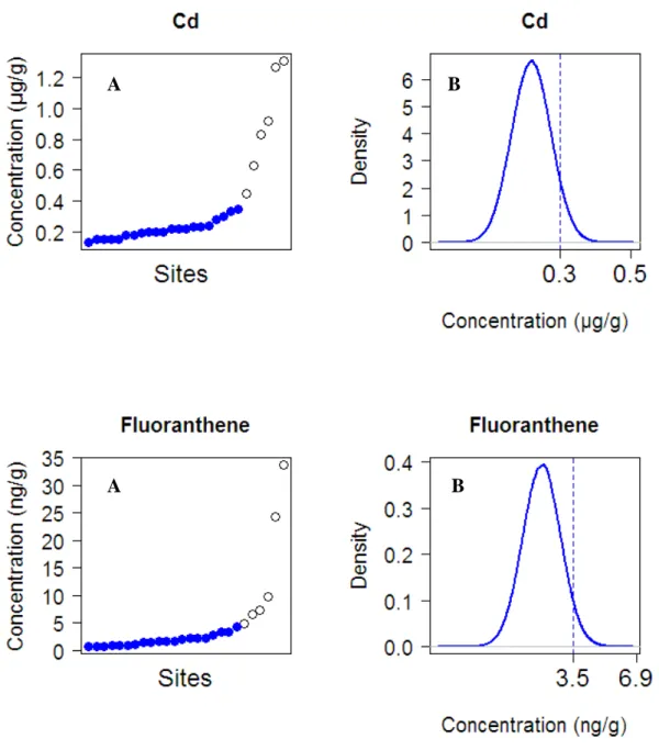
Figure 2. Example of the threshold value calculation for cadmium and fluoranthene, using the
proposed statistical approach (see section 2.5.1.for details). A: cadmium / fluoranthene concentrations measured in G. fossarum at each site, sorted by increasing values. B:
Distribution of the full circles of graph A constituting the larger data set following a Gaussian distribution; the threshold value derived with this method for cadmium and fluoranthene is indicated with the dotted line (percentile 95%).
A B
B A
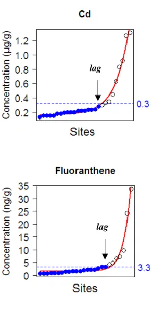
Figure 3. Example of the threshold value calculation for cadmium and fluoranthene,
determined using the model fit (Baranyi’s model). Concentrations measured at each site are sorted by increasing values. Fit of the Baryani’s model is showed in plain line. The lag is the break point where the accumulation enters an exponential phase; the concentration
corresponding to the lag is defined as the threshold value. The full circles are the sites below the lag, representing the background contamination in organisms.
lag lag
Table 1. Metal concentrations, limits of quantification (LQ) and frequency of quantification
(% data ≥ LQ) in caged Gammarus fossarum after 7 days of exposure for the 27 studied sites. Concentrations are expressed in µg.g-1 dw (dry weight). Med, Min and Max are the median, minimal and maximal of the measured concentrations, respectively.
Concentration (µg.g –1 dw)
Metals
Med Min Max Max/Min LQ
Frequency (%) Cd 0.22 0.13 1.31 10.4 0.04 100 Pb 0.28 0.14 1.39 9.9 0.07 93 Hg 0.049 0.040 0.107 2.7 0.010 100 Ni 0.48 0.27 1.29 4.8 0.19 85 Ag < LQ < LQ < LQ - 0.80 0 As 1.62 0.95 2.72 2.9 0.20 100 Cr 0.48 0.20 1.06 5.3 0.20 70 Cu 72.1 50.7 85.3 1.7 0.20 100 Co 0.32 0.13 0.96 7.4 0.08 100 Se 2.05 1.28 2.58 2.0 0.40 100 Zn 69.7 49.5 81.9 1.6 0.74 100
Table 2. Concentrations of organic substances, limits of quantification (LQ) and frequency of
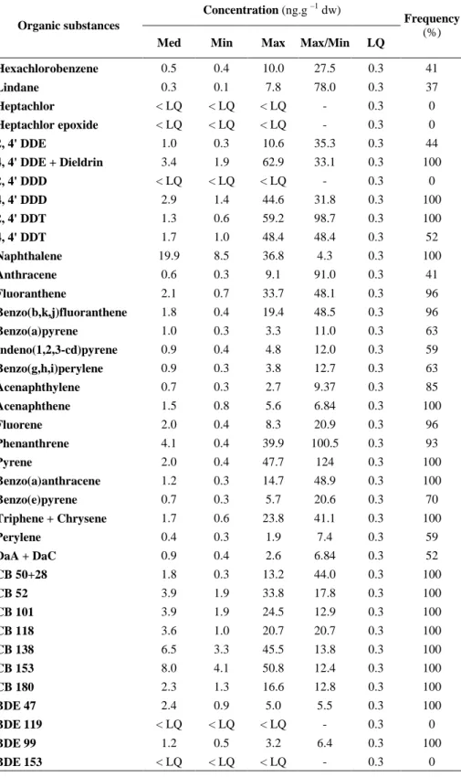
quantification (% data ≥ LQ) in caged Gammarus fossarum after 7 days of exposure for the 27 study sites. Concentrations are expressed in ng.g-1 dw. Med, Min and Max are respectively the median, minimal and maximal of the measured concentrations.
Concentration (ng.g –1 dw)
Organic substances
Med Min Max Max/Min LQ
Frequency (%) Hexachlorobenzene 0.5 0.4 10.0 27.5 0.3 41 Lindane 0.3 0.1 7.8 78.0 0.3 37 Heptachlor < LQ < LQ < LQ - 0.3 0 Heptachlor epoxide < LQ < LQ < LQ - 0.3 0 2, 4' DDE 1.0 0.3 10.6 35.3 0.3 44 4, 4' DDE + Dieldrin 3.4 1.9 62.9 33.1 0.3 100 2, 4' DDD < LQ < LQ < LQ - 0.3 0 4, 4' DDD 2.9 1.4 44.6 31.8 0.3 100 2, 4' DDT 1.3 0.6 59.2 98.7 0.3 100 4, 4' DDT 1.7 1.0 48.4 48.4 0.3 52 Naphthalene 19.9 8.5 36.8 4.3 0.3 100 Anthracene 0.6 0.3 9.1 91.0 0.3 41 Fluoranthene 2.1 0.7 33.7 48.1 0.3 96 Benzo(b,k,j)fluoranthene 1.8 0.4 19.4 48.5 0.3 96 Benzo(a)pyrene 1.0 0.3 3.3 11.0 0.3 63 Indeno(1,2,3-cd)pyrene 0.9 0.4 4.8 12.0 0.3 59 Benzo(g,h,i)perylene 0.9 0.3 3.8 12.7 0.3 63 Acenaphthylene 0.7 0.3 2.7 9.37 0.3 85 Acenaphthene 1.5 0.8 5.6 6.84 0.3 100 Fluorene 2.0 0.4 8.3 20.9 0.3 96 Phenanthrene 4.1 0.4 39.9 100.5 0.3 93 Pyrene 2.0 0.4 47.7 124 0.3 100 Benzo(a)anthracene 1.2 0.3 14.7 48.9 0.3 100 Benzo(e)pyrene 0.7 0.3 5.7 20.6 0.3 70 Triphene + Chrysene 1.7 0.6 23.8 41.1 0.3 100 Perylene 0.4 0.3 1.9 7.4 0.3 59 DaA + DaC 0.9 0.4 2.6 6.84 0.3 52 CB 50+28 1.8 0.3 13.2 44.0 0.3 100 CB 52 3.9 1.9 33.8 17.8 0.3 100 CB 101 3.9 1.9 24.5 12.9 0.3 100 CB 118 3.6 1.0 20.7 20.7 0.3 100 CB 138 6.5 3.3 45.5 13.8 0.3 100 CB 153 8.0 4.1 50.8 12.4 0.3 100 CB 180 2.3 1.3 16.6 12.8 0.3 100 BDE 47 2.4 0.9 5.0 5.5 0.3 100 BDE 119 < LQ < LQ < LQ - 0.3 0 BDE 99 1.2 0.5 3.2 6.4 0.3 100 BDE 153 < LQ < LQ < LQ - 0.3 0
37
Table 3. Calculated threshold values of bioavailable contamination determined by two
1
different approaches, a statistical approach and a model fit (see section 2.5); and threshold 2
validity (see section 4.3.). Threshold values are expressed in µg.g–1 dw for metals and in ng.g– 3
1
dw for organic substances. 4
38 5 6 7 8 9 10 11 12 13 14 15 16 17 18 19 20 21 22 23 24 25 26 27 28 29 30 31 32 33 34 35 36 nd: not determined. 37
Treshold values Threshold validity
Investigated substances Statistical
approach Model fit
Reliability ratio Validity Cd 0.3 0.3 0.00 valid Pb 0.4 0.3 0.07 valid Hg 0.06 0.09 0.30 valid Ni 0.7 0.7 0.00 valid As 2.5 nd nd not valid Co 0.5 0.5 0.00 valid Cr 0.9 nd nd not valid Cu 73.9 nd nd not valid Se 2.5 nd nd not valid Metals (µg.g–1 dw) Zn 84.7 nd nd not valid Hexachlorobenzene 0.6 1.0 0.04 valid Pesticides (ng.g–1 dw) Lindane 0.4 0.7 0.04 valid 2,4' DDE 1.9 1.6 0.03 valid
4, 4' DDE + Dieldrine 4.8 6.0 0.02 valid
4, 4' DDD 3.9 5.0 0.02 valid
2, 4' DDT 1.6 3.1 0.03 valid
DDTs
(ng.g–1 dw)
4, 4' DDT 2.8 3.2 0.01 valid
Naphthalene 32.7 nd nd not valid
Anthracene 1.5 1.3 0.02 valid
Fluoranthene 3.5 3.3 0.01 valid
Benzo (b,k,j) fluoranthène 3.8 3.1 0.04 valid
Benzo(a)pyrène 1.3 0.9 0.12 valid
Indeno (1,2,3-cd) pyrene 1.7 1.6 0.02 valid Benzo (g,h,i) perylene 1.3 1.1 0.05 valid
Acenaphtene 2.6 2.7 0.02 valid Acenaphtylene 1.3 0.9 0.15 valid Fluorene 2.9 1.6 0.16 valid Phenanthrene 6.8 3.7 0.08 valid Pyrene 3.3 3.1 0.00 valid Benzo(a)anthracene 2.2 1.8 0.03 valid Benzo(e)pyrene 1.3 1.1 0.04 valid Triphene+chrysene 2.6 2.9 0.01 valid
DaA-DaC 1.6 nd nd not valid
HAPs (ng.g–1 dw) Perylene 0.3 0.6 0.16 valid 50 + 28 3.5 2.9 0.05 valid 52 4.9 7.9 0.01 valid 101 5.8 6.6 0.03 valid 118 5.5 4.3 0.06 valid 138 8.3 10.9 0.06 valid 153 11.5 13.3 0.04 valid PCBs (ng.g–1 dw) 180 3.3 3.8 0.03 valid 47 4.3 nd nd not valid PBDEs (ng.g–1 dw) 99 2.1 1.1 0.30 valid
39
Table 4. Classification of study sites using the threshold values defined with the model fit approach. Grey squares indicate concentrations in
gammarids higher than the threshold value (values are given in µ g.g-1 dw for metals and in ng.g-1 dw for organics). Sites numbered from 1 to 12 are those considered as non subjected to anthropic activities with reference to the expert classification made by the Water Agency. Sites
numbered from 13 to 27 are those considered as subjected to anthropic activities with reference to the expert classification made by Water Agency (see section 2.3).
40 Cd 0.83 1.31 1.27 0.18 0.15 0.15 0.17 0.23 0.23 0.22 0.63 0.2 0.45 0.33 0.21 0.19 0.12 0.15 0.28 0.24 0.3 0.91 0.21 0.14 0.2 0.2 0.35 Pb < LQ 0.17 0.31 0.22 0.16 0.14 0.14 0.43 0.19 0.27 0.46 0.85 < LQ 0.4 0.27 0.2 0.24 0.17 0.28 1.39 0.82 0.89 0.95 0.29 0.46 0.18 0.92 Hg 0.05 0.05 0.05 0.04 0.04 0.04 0.04 0.05 0.06 0.05 0.05 0.04 0.06 0.05 0.05 0.05 0.04 0.05 0.11 0.05 0.05 0.05 0.05 0.05 0.05 0.05 0.05 Ni 0.53 1.28 0.43 0.6 0.68 0.33 0.26 <LQ <LQ 0.5 0.35 0.45 0.48 1.27 0.37 0.37 0.34 0.59 0.88 0.45 <LQ <LQ 1.01 0.69 0.58 0.4 0.36 Co 0.33 0.23 0.27 0.33 0.13 0.14 0.14 0.47 0.27 0.31 0.33 0.39 0.46 0.32 0.28 0.27 0.29 0.26 0.96 0.24 0.43 0.44 0.5 0.39 0.36 0.23 0.34 Hexachlorobenzene 0.4 <LQ <LQ <LQ 0.4 0.5 <LQ <LQ <LQ 0.4 <LQ 0.9 < LQ < LQ < LQ < LQ < LQ < LQ 10.0 < LQ < LQ < LQ < LQ 0.6 < LQ 0.6 0.5 Lindane 0.3 <LQ <LQ <LQ <LQ <LQ <LQ <LQ 0.4 <LQ <LQ <LQ 0.3 0.4 0.4 < LQ 0.4 < LQ 7.8 0.4 <LQ 0.4 1.4 <LQ 0.6 < LQ < LQ 2, 4' DDE <LQ <LQ <LQ <LQ <LQ <LQ <LQ <LQ <LQ <LQ <LQ 1.7 0.3 1.1 1.5 < LQ 0.6 0.3 10.6 < LQ < LQ 0.4 2.1 0.9 1.0 < LQ 0.7 4, 4' DDE+Dieldrin 2.4 2.9 2.6 2.5 3.2 2.3 2.4 1.9 2.3 2.3 3.9 3.4 4.2 4.2 3.3 3.1 3.6 3.5 37.0 3.9 3.9 6.9 5.5 5.1 3.4 10.4 62.9 4, 4' DDD 2.0 1.9 1.9 1.9 1.9 2.0 2.3 1.6 2.4 2.1 3.6 3.7 1.4 3.5 2.3 3.0 1.8 3.3 44.6 3.4 2.9 4.3 6.3 5.2 3.3 5.9 24.3 2, 4' DDT 1.0 1.0 1.0 1.0 1.1 0.8 0.9 0.6 0.8 0.7 0.9 1.3 2.2 1.3 3.1 2.9 2.3 2.6 59.2 2.3 2.3 2.4 2.3 1.9 1.5 1.2 2.8 4, 4' DDT <LQ <LQ <LQ <LQ <LQ <LQ <LQ <LQ <LQ <LQ <LQ <LQ 1.2 1.3 1.7 1.9 1.7 1.7 48.4 2.8 2.3 2.1 2.9 1.4 1.0 <LQ 12.5 Anthracene <LQ <LQ 0.7 <LQ 0.4 <LQ <LQ <LQ <LQ <LQ <LQ 1.7 <LQ <LQ 0.5 1.0 <LQ 0.3 <LQ 0.9 <LQ 0.7 3.7 9.1 0.4 0.3 1.2 Fluoranthene 0.9 0.7 1.4 1.7 1.6 1.0 0.8 1.2 <LQ 1.0 1.7 7.3 0.7 2.0 3.4 2.3 3.4 2.9 1.5 6.5 2.3 4.8 33.7 24.2 4.3 2.3 9.8 Benzo(b,k,j)fluoranthene 0.4 0.6 1.0 1.2 1.7 <LQ 0.6 1.4 0.6 1.6 1.5 5.6 0.8 1.7 3.2 2.1 2.8 2.0 1.0 4.7 3.2 3.7 19.4 7.8 3.1 1.9 8.7 Benzo(a)pyrene <LQ <LQ <LQ 0.5 <LQ <LQ <LQ 0.5 <LQ <LQ 0.3 0.6 <LQ 1.1 1.0 0.9 1.1 0.7 <LQ 1.2 1.1 1.2 3.0 3.3 0.3 0.6 2.8 Indeno(1,2,3-cd)pyrene <LQ <LQ <LQ 0.5 0.4 <LQ <LQ <LQ <LQ <LQ <LQ 1.4 <LQ 0.5 0.9 0.9 1.0 0.7 <LQ 0.9 1.3 1.1 4.8 1.7 0.7 0.6 1.8 Benzo(g,h,i)perylene <LQ <LQ <LQ 0.3 0.4 <LQ <LQ 0.6 <LQ <LQ <LQ 1.6 <LQ 0.5 0.9 0.6 0.7 0.6 0.1 0.9 1.0 1.1 3.8 2.2 0.9 0.9 2.1 Acenaphthylene 0.4 0.5 0.3 <LQ 0.7 0.4 0.3 <LQ <LQ 0.3 0.3 0.9 0.6 0.6 0.9 <LQ 1.0 0.7 1.1 1.4 0.9 1.1 1.2 2.7 1.0 0.5 0.8 Acenaphthene 1.5 1.5 1.9 0.8 1.7 1.4 1.3 1.0 0.9 1.3 0.9 5.6 1.7 1.3 1.9 1.2 1.5 1.5 2.2 2.5 1.4 1.6 3.1 2.9 1.9 1.5 2.2 Fluorene 1.2 1.2 2.7 0.7 1.9 1.4 0.7 0.7 <LQ 0.5 0.6 6.1 2.6 1.8 2.2 1.5 2.0 2.1 2.6 2.7 1.4 2.4 8.3 6.5 4.8 0.4 5.1 Phenanthrene 2.2 2.0 8.7 2.1 4.4 3.5 0.6 2.1 <LQ 1.6 0.7 17.2 4.2 3.0 6.3 2.6 4.1 5.5 4.8 3.3 0.4 5.3 39.9 37.8 12.5 <LQ 26.6 Pyrene 0.7 0.5 2.1 1.1 1.3 0.5 0.8 1.1 0.4 1.2 1.5 6.0 0.8 2.1 2.4 1.9 2.6 3.0 2.0 8.0 2.0 4.1 40.7 47.7 5.4 2.9 10.8 Benzo(a)anthracene 0.6 0.3 0.6 0.9 0.8 0.5 0.6 1.0 0.3 0.6 0.8 2.2 0.6 1.3 1.8 1.3 1.5 1.2 1.1 4.8 1.9 2.2 14.7 11.4 2.4 1.3 3.9 Benzo(e)pyrene <LQ <LQ <LQ 0.3 0.4 <LQ <LQ 0.3 <LQ 0.4 0.4 1.5 <LQ 0.4 0.7 0.6 0.8 0.5 <LQ 1.2 0.9 1.1 5.7 2.6 0.9 0.7 2.3 Triphene + Chrysene 0.6 0.6 1.1 1.5 1.5 0.7 0.6 1.2 0.6 1.5 1.6 4.1 0.7 1.7 2.4 1.8 2.1 2.0 1.4 6.0 2.4 4.0 23.8 13.4 4.6 2.8 9.1 Perylene <LQ <LQ <LQ 0.3 0.4 <LQ <LQ 0.3 <LQ 0.4 0.4 1.5 <LQ 0.3 0.3 0.7 0.5 0.3 <LQ <LQ 0.3 0.5 1.2 0.8 0.4 0.3 1.9 PCB 50+28 2.0 1.6 1.6 1.5 3.8 1.8 0.6 0.3 1.0 1.6 0.6 5.9 1.2 2.2 2.1 1.1 2.9 1.8 13.2 1.2 0.7 1.5 4.7 3.2 5.3 2.6 2.3 PCB 52 3.9 2.6 3.5 3.5 4.2 2.7 2.5 2.7 2.7 3.9 2.4 8.6 4.1 7.7 9.8 2.2 4.3 3.8 33.8 3.2 1.9 2.7 8.3 4.6 9.4 3.9 5.6 PCB 101 3.9 4.7 3.6 3.8 3.9 2.3 2.9 1.9 2.6 3.6 3.3 9.3 3.7 9.8 13.5 2.7 4.0 3.7 24.5 5.0 3.6 7.3 14.9 7.6 8.7 4.8 4.8 PCB 118 2.9 3.4 2.7 3.5 2.7 1.4 1.2 <LQ 1.0 2.7 2.8 13.5 3.7 11.0 16.3 3.9 4.0 3.8 20.7 1.8 2.0 5.7 8.7 3.6 7.1 2.9 4.0 PCB 138 5.3 6.1 6.6 7.4 6.6 3.4 4.1 3.3 3.4 4.9 5.8 10.6 6.0 14.0 16.6 5.3 6.1 5.8 45.5 9.9 5.1 23.5 31.8 12.9 12.0 10.8 6.5 PCB 153 6.8 8.4 8.2 8.9 8.0 4.6 5.4 4.1 4.9 6.9 7.5 10.6 7.6 16.7 16.5 6.5 7.4 6.8 50.8 12.1 5.7 30.8 36.6 16.7 13.7 16.7 7.6 PCB 180 1.6 1.6 2.3 2.6 2.5 2.0 1.9 1.7 2.0 2.2 2.8 2.4 1.6 3.8 4.1 1.8 1.4 1.3 16.6 3.0 1.4 9.1 14.2 4.9 3.8 3.5 2.1 BDE 99 1.3 1.9 1.0 1.1 1.8 0.9 1.0 0.5 1.0 0.7 1.7 1.4 0.8 1.4 1.4 0.6 0.6 0.9 1.5 1.3 0.5 0.6 3.2 1.7 2.7 1.2 2.2
41 LQ: Limit of quantification
42
Table S1.Location and water physico-chemical characteristics for the 12 study sites selected among the national reference network (WFD
implementation). According to the expert classification of the Water Agency (i.e., no known anthropic pressure and overall good quality indices) these sites were considered not subjected by anthropic pressures.
For physicochemical characteristics, 2 values are given for each site. Except for temperature,these values correspond to measurements performed at the beginning and at the end of the exposure (i.e., at 7 days). Contrary to other parameters, temperature was measured every hour during the 7 days of exposure.
Site information Physicochemical characteristics
GPS coordinates Site
(river / location) E N Site code
Water temperature
(°C)
min – max [med]
Dissolved oxygen (%) pH Hardness (mg.L-1 of CaCO3) Doux Labatie d'Andaure 04°29′ 41.5" 45°01′ 23.6" 1 11.2 - 16.1 [14.0] 98 100 7.1 7.2 14.2 15.3 Cance
Saint Julien Vocance 04°30′ 11.9" 45°10′ 39.5" 2
9.8 - 15.2 [12.5] 100 100 7.0 6.6 16.1 17.2 Gier La Valla en Gier 04°30′ 36.4" 45°26′ 36.3" 3 9.9 - 14.2 [12.2] 100 100 7.2 6.5 16.5 16.9 Ain
Saint Maurice de Gourdans 05°11′ 20.0" 45°48′ 27.5" 4
12.2 - 16.1 [14.0] 99 100 8.0 8.3 173.4 164.9 Albarine Chaley 05°32′ 31.8" 45°57′ 22.8" 5 9.7 - 12.5 [11.0] 100 100 8.2 8.3 208.3 206.2 Mandorne Oncieux 05°28′ 23.7" 45°58′ 36.1" 6 8.7 - 13.0 [10.9] 100 99 8.2 8.3 157.6 157.5 Vareze Cours et Buis 04°58′ 52.0" 45°26′ 15.3" 7 10.4 - 15.3 [12.7] 100 100 7.9 7.9 180.9 168.1 Galaveyson
Saint Clair sur Galaure 05°07′ 50.3" 45°15′ 26.5" 8
10.2 – 14.7 [12.4] 100 100 7.8 7.5 163.7 173.1 Drevenne Rovon 05°27′ 55.5" 45°12′ 11.6" 9 10.6 - 14.7 [12.8] 100 100 8.2 8.3 175.1 176.6 Guiers Mort
Saint Laurent du Pont 05°45′ 17.4" 45°21′ 42.2" 10
8.6 - 10.7 [9.6] 100 100 8.4 8.5 172.3 175.7 Ardières Les Ardillats 04°31′ 15.9" 46°11′ 11.8" 11 8.9 - 14.5 [12.0] 100 100 7.9 8.2 43.7 39.7 Ergues
Poule les Echarmeaux 04°26′ 45.5" 46°08′ 21.2" 12
8.0 - 14.7 [11.6] 100 100 7.7 7.8 55.0 48.6
43 According to the expert classification of the Water Agency (i.e., degraded water chemical quality and/or degraded faunistic indices) these sites were considered subjected to anthropic pressures.
Site information Impact type Physicochemical characteristics
Site
(river / location) GPS coordinates Site code
Pressure type
and intensity Metals Pesticides
Other organic contami nants Water temperature (°C)
min – max [med]
Dissolved oxygen (%) pH Hardness (mg.L-1 of CaCO3) Doux
Saint Jean de Muzols
04°49′ 39.5" E 45°04′ 40.2" N 13 Industrial Agricultural Urban + + + 15.3 – 19.5 [17.0] 100 100 7.2 7.1 34.9 38.9 Cance Sarras 04°47′ 47.6" E 45°11′ 30.9" N 14 Industrial Urban + + + 12.0 – 17.6 [14.9] 100 100 7.7 7.6 118.7 126.5 Albarine Saint Rambert 05°26′ 01.8" E 45°56′ 32.1" N 15 Industrial 1 Urban 2 + 10.4 – 15.1 [12.7] 100 100 8.0 8.5 161.4 161 Veyle Lent 05°11′ 48.4" E 46°06′ 58.7" N 16 Agricultural 3 ++ 11.1 – 14.1 [12.7] 100 98 8.0 7.8 231.1 244.4 Veyle Servas 05°10′ 31.3" E 46°07′ 37.9" N 17 Agricultural 3 +++ 11.0 – 16.4 [13.9] 100 86 8.3 7.9 228.7 227.9 Ange Brion 05°33′ 05.3" E 46°10′ 12.3" N 18 Industrial 3 Urban 2 ++ +++ 9.8 - 15.8 [12.8] 100 89 8.3 7.9 200.4 289.6 Drac Fontaine 05°42′ 04.3" E 45°11′ 36.6" N 19 Industrial 3 +++ +++ +++ 13.1 - 16.9 [15.4] 100 100 7.9 7.9 130.5 164.6 Turdine Arbresle 04°36′ 09.1" E 45°50′ 15.5" N 20 Industrial 3 Urban + + 10.0 - 17.0 [13.6] 100 100 8.4 8.2 174.1 165.6 Azergues Legny 04°34′ 21.4" E 45°54′ 24.6" N 21 Agricultural 2 Industrial 2 Urban +++ + 11.5 - 15.4 [12.9] 100 100 8.1 8.1 133.2 133.2 Azergues Lucenay 04°43′ 33.1" E 45°54′ 41.5" N 22 Agricultural 3 Industrial 2 +++ +++ + 13.3 - 18.2 [15.8] 100 100 8.1 8.1 256.2 268.5 Gier Givors 04°45′ 42.3" E 45°35′ 15.4" N 23 Urban ++ + ++ 11.8 - 19.2 [16.7] 100 100 7.2 7.6 204.0 143.5 Rhône Givors 04°47′ 03.4" E 45°35′ 36.4" N 24 Urban Industrial ++ + ++ 18.0 - 19.8 [19.2] 100 100 7.7 7.6 188.6 190.0 Bourbre Pont de Cheruy 05°10′ 29.9" E 45°04′ 00.3" N 25 Urban 2 Industrial 2 + + + n.a. 100 100 7.7 7.4 230.4 260.6 Saône Ile Barbe 04°49′ 57.3" E 45°47′ 49.4" N 26 Urban Industrial ++ +++ + 18.5 - 19.8 [18.8] 100 100 7.9 7.7 110.2 235.4 Ardières
Saint Jean d’Ardières
04°44′ 00.9" E 46°07′ 18.4" N 27 Agricultural 3 Industrial 2 Urban +++ +++ ++ 12.7 - 15.6 [14.3] 100 100 8.2 8.9 n.a. 106.1
44 Impact type: + indicate the pressure’s intensity (+: low; ++: moderate; +++: strong).
Values displayed in the column “pressure type and intensity” indicate, when available, the impact level of the selected contaminants on the receiving environment (1: moderate; 2: moderate to strong; 3: strong). These values were defined regarding data on land use, chemical monitoring and ecological diagnosis (http://www.rhone-mediterranee.eaufrance.fr/gestion/dce/documents-locaux.php)
For physicochemical characteristics, 2 values are given for each site. Except for temperature,these values correspond to measurements performed at the beginning and at the end of the exposure (i.e., at 7 days). Contrary to other parameters, temperature was measured every hour during the 7 days of exposure.
45
Figure S1. Survival rate (mean ± standard deviation of 4 replicates) of caged G. fossarum
after 7 days of exposure for all studied sites (n=27)
0 10 20 30 40 50 60 70 80 90 100 1 2 3 4 5 6 7 8 9 10 11 12 13 14 15 16 17 18 19 20 21 22 23 24 25 26 27 Study sites S ur v iv a l ra te ( % )
47
Figure S2. Threshold values determined for investigated metals and organic substances. For
each substance, the top figure gives the threshold value determined with the model fit (Baranyi’s bacterial growth model), and the bottom figure, the threshold value determined with the statistical approach (normality assumption).
Threshold values are given in µg.g-1 (dry weight) for metals and in ng.g-1 (dry weight) for organic substances.
53
II. ORGANOCHLORINE PESTICIDES
55 opDDE: 2,4’-DDE