HAL Id: hal-01187745
https://hal.archives-ouvertes.fr/hal-01187745
Submitted on 27 Aug 2015
HAL is a multi-disciplinary open access
archive for the deposit and dissemination of
sci-entific research documents, whether they are
pub-lished or not. The documents may come from
teaching and research institutions in France or
abroad, or from public or private research centers.
L’archive ouverte pluridisciplinaire HAL, est
destinée au dépôt et à la diffusion de documents
scientifiques de niveau recherche, publiés ou non,
émanant des établissements d’enseignement et de
recherche français ou étrangers, des laboratoires
publics ou privés.
Nicolas Berthier, Xin An, Hervé Marchand
To cite this version:
Nicolas Berthier, Xin An, Hervé Marchand. Towards Applying Logico-numerical Control to
Dy-namically Partially Reconfigurable Architectures. 5th IFAC International Workshop On Dependable
Control of Discrete Systems - DCDS’15, May 2015, Cancun, Mexico. pp.132-138. �hal-01187745�
Towards Applying Logico-numerical
Control to Dynamically Partially
Reconfigurable Architectures
Nicolas Berthier∗ Xin An∗∗ Herv´e Marchand∗
∗INRIA Rennes - Bretagne Atlantique, Rennes, France ∗∗Hefei University of Technology, Hefei, China
Abstract: We investigate the opportunities given by recent developments in the context of Discrete Controller Synthesis algorithms for infinite, logico-numerical systems. To this end, we focus on models employed in previous work for the management of dynamically partially reconfigurable hardware architectures. We extend these models with logico-numerical features to illustrate new modeling possibilities, and carry out some benchmarks to evaluate the feasibility of the approach on such models.
Keywords: Discrete Controller Synthesis, Infinite Systems, Control of Computing, Synchronous Languages, Hardware Architectures, Dynamically Partially Reconfigurable FPGA
1. INTRODUCTION
Recent proposals by Berthier and Marchand (2014) in the domain of symbolic Discrete Controller Synthesis (DCS) techniques have led to the development of a tool capable of handling logico-numerical systems and properties, i.e., involving state variables defined on infinite domains. The handling of such infinite systems opens the way to new opportunities for modeling and control, that still need to be investigated.
We extend real-life models proposed by An et al. (2013a,b) for the management of Dynamically Partially Reconfig-urable (DPR) hardware architectures to: (i) assess the feasibility of the proposal on bigger systems, (ii) perform some performance evaluations of the new tool ReaX on realistic models, including for control objectives newly im-plemented in this tool; and (iii) introduce logico-numerical features in the model to assess that the approach can still be applied using models involving quantitative aspects.
DPR Hardware Architectures DPR hardware
architec-tures, typically Field Programmable Gate Arrays (FPGAs) (Lysaght et al., 2006), have been identified as a promising solution for the design of energy-efficient embedded systems (Hinkelmann et al., 2009). However, such solutions have not been extensively exploited in practice for two main reasons: i) the design effort is extremely high and strongly depends on the available chip and tool versions, and ii) the simulation process, which is already complex for non-reconfigurable systems, is prohibitively large for reconfig-urable architectures. Therefore, new adequate methods to deal with their correct dynamical reconfiguration are required to fully exploit their potential.
Dynamical reconfiguration management requires choosing new configurations depending on the history of events occur-ring in the system and predictive knowledge about possible outcomes of reconfigurations. Such decision-making compo-nent is difficult to design because of the combinatorics of
possible choices, the transversal constraints between them, and even more, the history aspects. The work we present advocates the application of DCS techniques to fulfill this control problem.
Related Works The reconfiguration management in DPR
technologies is usually addressed by using manual encoding and analysis techniques that are tedious and error-prone according to G¨ohringer et al. (2008). Other existing approaches dedicated to self-management of adaptive or reconfigurable systems use heuristics and machine learning techniques (Sironi et al., 2010; Paulsson et al., 2006; Jovanovi´c et al., 2008) for instance. Maggio et al. (2012) discuss some approaches applying standard control
techniques such as Proportional Integral and Derivative (PID) controller or Petri nets-based control. The same kind of control has also been used for processor and bandwidth allocation in servers (Lu et al., 2002). Eustache and Diguet (2008) applied close-loop control to select hardware/software configurations on an FPGA with a configuration control based on a data-flow model and diffusion mechanisms. We note that such a solution relies on heuristics and empirical laws that prevent instability and select the suitable configurations.
Compared to the above reconfiguration control techniques, major advantages of the discrete control approach consid-ered by An et al. (2013a,b) are the enabled formal correct-ness and guarantees on run-time performance, as well as the possibility to synthesize the controller automatically. Outline We first present in Section 2 the modeling for-malism we use for expressing the reconfiguration problem, as well as the tools involved in our work. Sections 3 detail the problem of reconfiguration control for FPGA-based DPR systems. We expose the modeling and formulation as a DCS problem, as well as an illustrative logico-numerical extension of the model in Section 4, and we report on our performance evaluation experiments in Section 5.
2. MODELING FORMALISM AND TOOLS 2.1 Arithmetic Symbolic Transition Systems
The model of Arithmetic Symbolic Transition Systems (ASTSs) is a transition system with (internal or input) variables whose domain can be infinite, and composed of a finite set of symbolic transitions. Each transition is guarded on the system variables, and has an update function indicating the variable changes when a transition is fired. This model allows the representation of infinite systems whenever the variables take their values in an infinite domain, while it has a finite structure and offers a compact way to specify systems handling data.
Let V = hv1, . . . , vni be a tuple of variables and Dv the
(infinite) domain of v. We note DV = Qi∈[1,n]Dvi the
(infinite) domain of V . vi(V ) gives the value of variable vi
in vector V .
Definition 1. (Arithmetic Symbolic Transition System). An ASTS is a tuple S = hX, I, T, A, Θ0i where:
• X = hx1, . . . , xni is a vector of state variables ranging
over DX = Qj∈[1,n]Dxj and encoding the memory
necessary for describing the system behavior;
• I = hi1, . . . , imi is a vector of variables that ranges
over DI =Qj∈[1,m]Dij, called input variables;
• T is of the form (x0
i:= Txi)xi∈X, such that, for each
xi ∈ X, the right-hand side Txi of the assignment
x0i := Txi is an expression on X ∪ I. T is called the
transition function of S, and encodes the evolution of the state variable xi. It characterizes the dynamic of
the system between the current state and the next state when receiving an input vector.
• A is a predicate with variables in X ∪ I encoding an assertion on the possible values of the inputs depending on the current state;
• Θ0 is a predicate with variables in X encoding the set
of initial states.
For technical reasons, we shall assume that A is expressed in a theory that is closed under quantifier elimination as for example the Presburger arithmetic.
ASTSs can conveniently be represented as parallel compo-sitions of Mealy automata with numerical variables and explicit locations or in its symbolic form.
Let us consider the following example ASTS where X = hξ, x, oi, I = ha, ii with DX= {F, G} × Z × B, DI = B × Z
T = ξ0:= G if (ξ = F ∧ a ∧ x ≥ 0), F if (ξ = G ∧ i > 42), ξ otherwise x0 := 2x + 1 if (ξ = F ∧ a ∧ x ≥ 0), i if (ξ = G ∧ i ≤ 42), x otherwise o0 := (ξ = F ∧ a ∧ x ≥ 0) ∨ (ξ = G ∧ i > 42) A(hξ, x, o, a, ii) = (ξ = G ∧ 3x + 2i ≤ 41 ∧ a) Θ0(hξ, x, oi) = (ξ = F ∧ x = 0)
The corresponding Mealy automaton with explicit locations (leaving A aside) can be represented as in Figure 1.
Remark 1. Observe that the variable o is actually an output of the system, although it belongs to the vector of state variables. Indeed, we do not distinguish between those two kinds of variables to keep the ASTS models simple. We
F G
a ∧ x > 0/o, x := 2x + 1
¬a ∨ x < 0 i > 42/o
i 6 42/x := i x := 0
Fig. 1. Example ASTS as a Mealy automaton.
can characterize output variables as the ones that never appear in the right hand side of the assignments in T . Remark 2. We qualify as logico-numerical an ASTS whose state (and non-output) and input variables are Boolean variables (B) or numerical variables (typically, R or Z), i.e., such that X = Bk∪ Rk0 ∪ Zk00 with k + k0+ k00= n
(and similarly for the input variables). ASTSs with only Boolean non-output state variables are called finite. To each ASTS, one can make correspond an Infinite Transition System (ITS) defined as follows:
Given an ASTS S = hX, I, T, A, Θ0i, we make correspond
an ITS [S] = hX , I, TS, AS, X0i where:
• X = DX is the state space of [S];
• I = DI is the input space of [S];
• TS ⊆ X × I → X is such that
TS(x, ν) = (x0j)j∈[1,n]⇔ ∀j ∈ [1, n], x0j:= Txj(x, ν);
• AS ⊆ X × I is such that
AS = {(x, ν) ∈ X × I|A(x, ν) = true};
• X0⊆ X is the set of initial states, and is such that
X0= {x ∈ X |Θ0(x) = true}.
The behavior of such a system is as follows. [S] starts in a state x0 ∈ X0. Assuming that [S] is in a state
x ∈ X , then upon the reception of an input ν ∈ I such that (x, ν) ∈ AS, [S] evolves in the state x0 = TS(x, ν).
We denote XTrace([S]) the set of states that can be reached in [S]. Given an ASTS S and a predicate Φ over X, we say that S satisfies Φ (noted S |= Φ) whenever XTrace([S]) ⊆ {x ∈ X |Φ(x) = true}.
Control of an ASTS Assume given a system S and a
predicate Φ on S. Our aim is to restrict the behavior of S by means of control in order to fulfill Φ. We distinguish between the uncontrollable input variables U which are defined by the environment, and the controllable input variables C which are defined/restricted by the controller of the system. For technical reason, we assume that the controllable variables are Boolean. Note that the partitioning of the input variables in S induces a “partitioning” of the input space in [S], so we have I = DU×
DC. A controller is then given by a predicate AΦ over
X ∪ U ∪ C that constrains the set of admissible (Boolean) controllable inputs so that the traces of the controlled system always satisfy Φ.
Definition 2. (Discrete Controller Synthesis Problem). Given an ASTS S = hX, U ∪ C, T, A, Θ0i and a predicate Φ
over X, solving the discrete controller synthesis problem is to compute a predicate AΦ such that
S0 = hX, U ∪ C, T, AΦ, Θ0i |= Φ
and ∀v ∈ X ∪ U ∪ C, AΦ(v) ⇒ A(v).
The general control problem that we want to solve is undecidable. In (Berthier and Marchand, 2014), we then used abstract interpretation techniques to ensure, at the price of some over-approximations, that the computation
of the controller terminates (see e.g., (Cousot and Cousot, 1977)). This over-approximation ensures that the forbidden states are not reachable in the controlled system. Thus, the synthesized controller remains correct, yet may not be maximally permissive w.r.t the invariant. For the details on how the controller is computed, one can refer to (Berthier and Marchand, 2014).
2.2 ReaX & BZR
ReaX Berthier and Marchand (2014) introduced the tool ReaX implementing the above symbolic algorithms for the synthesis of controllers ensuring safety properties of infinite state systems modeled by ASTSs. Compared with what is reported in this previous work, in addition to the invariance of a predicate, one can also request the controlled system to be deadlock-free. Adapting techniques from Marchand and Samaan (2000), ReaX also implements classical algorithms of invariance and reachability enforcement for finite sys-tems, as well as one-step optimization of numerical variables for general ASTSs.
BZR An et al. (2013a,b) used the reactive data-flow
language BZR (Delaval et al., 2010) to describe their solution. BZR programs are built as parallel compositions of data-flow nodes, each having input and output flows. The body of the node describes how input flows are transformed into output flows, in the form of a set of equations and/or automata. They are evaluated, all together at each step of a reactive system (hence the composition is called synchronous), by taking all inputs, computing the transitions and equations, and producing the outputs. An invariant and controllable variables can be specified, and the BZR compiler involves DCS to automatically produce a controller guarantying that the resulting controlled system satisfies the invariance property by constraining the values of the controllable variables. To do so, BZR involves a compilation phase using either Sigali (Marchand et al., 2000) or ReaX (Berthier and Marchand, 2014) DCS tools. Remark 3. As Sigali supports the handling of cost functions for optimization purposes (functions from the finite state space and input space of the systems to integers) (Marchand et al., 2000), the Sigali BZR backend is able to make use of this device to translate programs involving nodes with Integer output flows (Delaval et al., 2013). It is however unable to translate programs with Integer state variables, like the one of Figure 1.
3. FPGA CONTROL PROBLEM
We consider applications made of tasks executing according to dependency constraints on an FPGA platform. The latter may provide various computation resources having different characteristics or specializations for the tasks to execute, and each task may be implemented in several ways using dissimilar sets of resources.
An et al. (2013a,b) provided a solution for the problem of choosing a scheduling satisfying both the execution depen-dencies between the tasks and the utilization constraints on the resources of the FPGA platform. This proposal consists in the model-based generation of a run-time manager whose role is to start tasks and detect their termination, and allocate appropriate computation resources for them
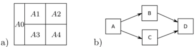
a) A0 A1 A2 A3 A4 b) B A C D
Fig. 2. a) Architecture; b) Application DAG specification. to execute. The run-time manager is designed by first modeling the platform and the task dependency graph using a synchronous language, and then solving a DCS problem to enforce the correct behavior of the whole system. We recall in this section the modeling principles employed in the previous work (An et al., 2013a,b) for the design of the run-time manager, and introduce the basis for the extension of the model with logico-numerical features. 3.1 Describing the System
Hardware We consider a multiprocessor architecture
implemented on a reconfigurable device (e.g., Xilinx Zynq) comprising a general purpose processor A0 (e.g., ARM core) executing the run-time manager. The device also includes a reconfigurable area (e.g., FPGA-like with power management capabilities) divided into reconfigurable tiles. Figure 2-a) shows an illustrative example comprising four tiles A1–A4. The communications between architecture components are achieved by means of a Network-on-Chip (NoC). Each processor and tile implements a NoC Interface (NI). Tiles can be combined and configured to implement
and execute tasks by loading predefined bitstreams. The FPGA platform is equipped with a battery supplying it with energy; this battery may be setup to enable harvesting. We also assume that the hardware platform provides means for the programs executing on the processor to measure its remaining capacity, either directly in the case of a smart battery (SBS Implementers Forum, 1998) if the platform is equipped with the appropriate devices, or indirectly, e.g., by interpretation of output voltage measurements. Regarding power management of the FPGA, any unused tile Ai can be put into sleep mode with a clock gating mechanism such that it consumes a minimum static power.
Application Software We consider that the application software is described as a directed acyclic graph (DAG), where nodes represent individual tasks to be executed, and directed edges depict dependency constraints between tasks: e.g., an edge between nodes A and B indicates that the task A must have terminated its execution before B can execute. Figure 2-b) shows an illustrative example consisting of four tasks A, B, C and D. Note that we do not restrict the abstraction level of tasks: they can denote atomic operations or coarse fragments of system functionality. The run-time manager is in charge of scheduling the tasks so that their execution dependencies are satisfied.
Given a hardware architecture, a task can be implemented in various ways, each having specific characteristics in terms of: (i) the set of tiles used for its execution; (ii) its wort case execution time; and (iii) peak power consumption. Before executing a task on a reconfigurable architecture, the task implementation must be loaded to reconfigure the corresponding tiles if required. This reconfiguration
task A or task B task C task B task C 1) 2) 3)
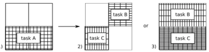
Fig. 3. Configurations and reconfigurations.
operation inevitably involves some overheads regarding, e.g., time and energy. For simplicity, we assume that the worst case execution time of each task implementation encompasses the time required to reconfigure the tiles it uses (as in the worst case, a task implementation must always be loaded before being executed).
Reconfiguration Figure 3 exemplifies three system con-figurations. In 1), task A is running on tiles A3 and A4 (see Figure 2-a)) while tiles A1 and A2 are in sleep mode.
Configurations 2) and 3) show two scenarios where tasks B and C run in parallel. Assume tasks B and C have two implementations so that the system can go to either 2) or 3) once task A finishes its execution (according to the graph of Figure 2-b)). If the current state of the battery level is low, the system would choose 2) as 3) requires the complete circuit surface and therefore consumes more power. On the contrary, when the battery level is high, 3) would be chosen if the user expects a better performance. 3.2 System-level Objectives
The run-time manager can decide to delay the execution of a task and determines which implementation of it to trigger. These choices are made according to system objectives that define the system functional and non-functional requirements. The objectives considered in this work, are either logical control or optimization objectives. Generally speaking, logical objectives express properties about discrete states of the system (e.g., mutual exclusions), whereas optimal ones concern weights and costs.
The logical control objectives we consider are: (i) exclusive uses of tiles A1–A4 by the executing tasks; (ii) switch tiles into active or sleep mode depending on whether a task executes on them or not to save energy; (iii) avoid power consumption peaks of the hardware platform w.r.t the electrical charge of the battery; and (iv) once started, the application can always finish. Optimization objectives notably encompass the minimization of the power peaks of the platform to augment the lifespan of the battery. 4. MODELING RECONFIGURATION CONTROL AS A
DCS PROBLEM
We focus on the management of computations on the tiles and dedicate the processor area A0 exclusively to the execution of the resulting run-time manager. So, we build a global system model as an ASTS representing the behavior of the reconfigurable computing system; system objectives are then specified using predicates expressed on variables of the model.
We recall, and reformulate in terms of ASTSs, the models proposed by An et al. (2013a,b). At the same time, we introduce a new, logico-numerical model for the battery, to demonstrate the added expressiveness allowed by the ASTSs handled by ReaX.
a) Acti Slei acti = true acti = false c_ai not c_ai c_ai acti RMi b) H M L down up up down down st=h st=m st=l st up BM
Fig. 4. Models RMifor a tile Ai, and BM for a battery.
4.1 System Model
Modeling the Tiles Figure 4-a) depicts the model describ-ing the behavior of a tile Ai: it features two states (Sle and Act) as a tile may or may not be active at a given instant. The model switches from a state to another depending on the value of its Boolean controllable variable c ai. The
output actirepresents its current mode.
Discrete Battery Model Figure 4-b) represents a discrete model for a battery proposed by An et al. (2013a,b). It is characterized with three states/levels: H (high), M (medium) and L (low). This model is assumed to take its inputs from a dedicated software executing on processor A0, that interprets capacity measurements and drives the state of this model by emitting up and down events depending on the current electrical charge of the battery. The output st ∈ {H, M, L} reflects the internal state of the model.
Logico-numerical Battery Model We now present a new
model for a smooth representation of the state of the battery in the system model. This model aims at illustrating the expressiveness of logico-numerical ASTSs handled by ReaX. This new model receives as input a rough measure cm of
the actual electrical charge (e.g., in Coulombs) provided by a dedicated sensor, and an estimation ceof the capacity
spent since the last reaction of the model. The state of the battery in this model consists in a numerical variable c providing an estimation of the remaining capacity of the battery. The domain of c can be the domain of reals (arbitrary-precision rationals actually).
At each reaction of the model, the value of c is estimated by using some sort of exponentially weighted moving average: it is computed by using cmwhen the input measurement
from the sensor is determined as valid by bounding its absolute difference with the estimated capacity c; the model tries to estimate this value by other means otherwise. The model is further parameterized with a constant smoothing factor α ∈ [0, 1] that specifies the impact of the variations of cm on the state variable c. The constant β serves as a
bound to determine the validity of the measured input. Although the value of c could be used directly in the definition of logical control predicates (and possibly op-timization objectives), e.g., to decide whether a given power consumption peak is admissible by the battery, for illustrative purposes we use it directly to compute a value for the finite output st based on additional constant threshold electrical charges λ and µ. In this way, this new battery model is interchangeable with the discrete one, and system control and optimization objectives can be reused whatever the chosen battery model.
The assignment of state variable c and output st ∈ {H, M, L} can be expressed as
I req/rA A eA/rB,rC B,C D eD/end T eA,eB,eC,eD rA,rB,rC,rD C eB and eC/rD eB eC eC/rD B eB/rD req Sdl end
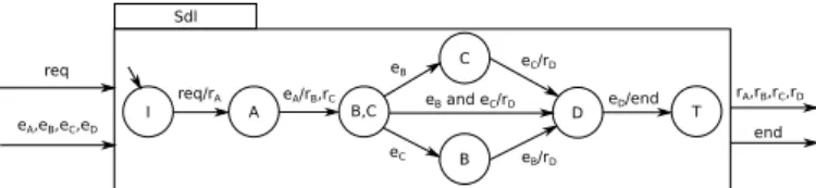
Fig. 5. Application DAG execution behaviors.
WA IA XA1 XA2 rA, c1 rA, c2 rA, not c c2 eA eA c1 ({A1}, 200,180) ({A3,A4}, 100,250) ({},0,0) ({},0,0) TMA rA eA c1,c2 esA esA=XA1 esA=W esA=XA2 esA=I rsA,wtA,ppA
Fig. 6. Model TMA of task A.
c0:= (c − ce)(1 − α) + cmα if |c − cm| < β (c − ce) otherwise st0 := L if c06 λ, M if λ < c0 6 µ, H otherwise and c can be initialized using a predefined constant value or with the first input measure cm, assuming it is valid
(in the latter case, the model would become slightly more complex). c is indeed a state variable of the model, as it appears in its own assignment expression.
Note that cemay be an input of the whole system model,
or even be computed by using another numerical variable keeping track of estimated power consumption peaks, plus a measure of the time elapsed since the last reaction. Encoding the Task Graph The software application is de-scribed by its task graph, i.e., as a DAG specifying the tasks to be executed, as well as their execution dependencies. This DAG is encoded as a scheduler automaton representing all possible execution scenarios. It does so by keeping track of application execution states and emitting appropriate start requests in reaction to tasks’ finish notifications. Figure 5 shows the scheduler automaton of the application DAG in Figure 2-b). When in idle state I and upon receipt of application request event req, it requests the start-up of task A by emitting event rA. Upon receipt of eA notifying
the termination of A’s execution, events rB and rC are
emitted together to request start-up of tasks B and C (that will then potentially execute in parallel). Task D is not requested until the execution of both B and C is finished, respectively denoted by events eB and eC. The scheduler
then reaches the final state T and emits event end, implying the end of the application’s execution, upon receipt of eD.
Remark 4. Note that several scheduler automata like the one of Figure 5 can be composed in a hierarchical way to describe complex task graphs. Using a sub-scheduler X, this composition operation only requires to bind a task start request (say, rX) with X’s req input, and conversely its
termination notification (end) to the corresponding task termination request (eX).
Task Model One can distinguish several stages during a tasks’ lifetime (see Section 3.1): not scheduled for execution; scheduled but not executing; and having the tiles configured with one of its implementation and executing.
We consequently model tasks with automata, such as the one of Figure 6 for A: it features idle and waiting states IA and WA, plus as many execution states as available
implementations of A (X1A and X2A). Controllable variables c1and c2are integrated in the model to encode the choices
given to the run-time manager; e.g., from the idle state, it can then choose to delay the execution of a task, or to select and start the execution of one of its implementation. The output esA reflects the execution state of the task.
Three observations of interest are considered for each task. For a task t, we capture them by associating a tuple (rst, wtt, ppt) to the states of task models, where: rst∈ 2RA
(RA being the set of architecture resources — i.e., the tiles in our case), wtt ∈ N and ppt ∈ N are the WCET
and the peak power consumption for the task’s state. The observations associated with executing states are the values associated with their corresponding implementations. For idle and wait states, rst= ∅, wtt= 0, ppt= 0.
Remark 5. Task observation variables defined in this sec-tion are outputs of the model, and hence belong to the vector of state variables X in the corresponding ASTS model (see Remark 1): the fact that the domain of some of them is infinite does not make the ASTS’s state space infinite. Global System Model The whole system model represents all the possible system execution behaviors in the absence of control (i.e., if a run-time manager is not yet integrated). In our example case of four tiles and set Tasks = {A, B, C, D} of tasks, it comprises the parallel composition of the sub-models for tiles RM1–RM4, battery BM and tasks TMA–
TMD, plus a scheduler Sdl encoding the task graph:
S = RM1|| . . . ||RM4||BM||TMA|| . . . ||TMD||Sdl.
In terms of ASTSs, and assuming variable names do not clash between the various sub-models of the system, this parallel composition essentially boils down to con-catenate together, for each sub-model m: the vectors of state variables Xm’s, controllable (resp. non-controllable)
inputs Cm’s and Um’s, and assignments Tm’s. The global
assumption A made about the environment is the con-junction of all assumptions of the sub-models Am’s. As
for the initial state, the predicate Θ0 is defined so that
X0= {hSle1, . . . , Sle4, H, IA, . . . , ID, Ii}.
Global Observations The observations output locally by each sub-model (e.g., task models) need to be combined into a set of global values in order to account for the resource consumption of the whole system. These values constitute the global observations of the model based on which logical control and optimization objectives can be expressed. In our case, the global observations available for a particular operating state of the system is the tuple of variables (rs, wt, pp) whose values are computed based on the indi-vidual tasks’ observations at the current reaction (denoted rs0t, wt0tand pp0t). Global observation variables are added to the vector of state variables as any other outputs, and are computed by adding corresponding assignments in T as follows: rs0 :=[ t∈Tasksrs 0 t wt0 := min t∈Tasks{wt 0 t| wt 0 t6= 0} if defined, 0 otherwise pp0 :=X t∈Taskspp 0 t
Note that in the assignments above, primed versions of tasks’ observations are actually substituted in the ASTS model by the expression they are respectively assigned to. Remark 6. By construction, global observation values are outputs of the system and can be computed as functions defined on its state only.
4.2 System Objectives
Based on the model described above, we can formalize the objectives of Section 3.2 in terms of the states and observations defined on the states.
The logical control objectives to be enforced on the system by the run-time manager can be expressed by using two predicates Φ : DX → B and χ : DX → B, respectively
encoding invariance and reachability requirements, and expressed on state variables. Φ can be expressed as a conjunction, each of its conjuncts encoding one aspect of the logical control needs:
• exclusive use of tiles: Φx(X) = ∀(s, t) ∈ Tasks2, s 6=
t, rss(X) ∩ rst(X) = ∅;
• shut-down and start-up of tiles depending on whether they are used or not by an executing tasks’ imple-mentation: Φa(X) = (∀a ∈ rs(X), acta = true) ∧
(∀a ∈ Drs\ rs(X), acta = false);
• given a mapping ppthr : {L, M, H} → N from discrete battery levels to threshold peak power values, con-straining the total power peak depending on the level of the battery: Φp(X) = pp(X) 6 ppthr (st(X)).
In turn, the reachability predicate χ specifies that a state must be reachable where the value of the output end of Sdl is true (meaning that the application has finished its execution): χ(X) = (end(X) = true).
One-step optimal objectives aim at minimizing or maximiz-ing numerical state variables in a smaximiz-ingle step. Optimization objective of Section 3.2 belongs to this type, by requesting to select successor states minimizing power peaks pp. 4.3 Solving the DCS Problem and Using the Result All the ASTS models above except the logico-numerical battery model are finite ASTSs as their non-output state space is finite (i.e., numerical state variables are outputs, and can thus be represented a cost functions associating numerical values to discrete states — see Remarks 1, 5 and 6). Thus, one can write these models in BZR, use either the Sigali or the ReaX backend of the compiler, solve the resulting DCS problem, and then automatically obtain a controller satisfying the system objectives. Associated with the model, this controller can be used by the run-time manager to dynamically reconfigure the system.
5. EVALUATION & EXPERIMENTAL RESULTS We report in this section our experiments to evaluate the efficiency of ReaX to solve DCS problems on models as described above. All executions were performed on a 3.2GHz Intel® Xeon®multi-core1 processor with about 6GB of main memory. We first show comparisons of Sigali w.r.t ReaX in the case of finite models, and then present performance results of ReaX on logico-numerical ASTSs.
1 Note however that both Sigali and ReaX are single-threaded.
50ms ¼s 1s 5s 15s 60s 5m ¼h 1h 2 3 4 5 6 7 8 9 10 11 Syn thesi s Time Number of Tasks Sigali ReaX
Fig. 7. Synthesis times for generated benchmarks.
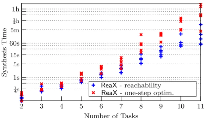
¼s 1s 5s 15s 60s 5m ¼h 1h 2 3 4 5 6 7 8 9 10 11 Syn the sis Time Number of Tasks ReaX - reachability ReaX - one-step optim.
Fig. 8. Synthesis times of ReaX for invariance and either reachability enforcement or one-step optimization. Logical Control: Efficiency of ReaX w.r.t Sigali A per-formance evaluation of Sigali for solving reconfiguration control problems similar to the ones considered in this paper has already been presented by An et al. (2013a). In order to compare the benefits of using ReaX w.r.t Sigali for the same kind of problems, we conducted extensive experiments based on multiple instances of the reconfiguration control problem. Each one of these models is built based on a randomly generated hierarchical task graph constructed recursively by exploiting the idea mentioned in Remark 4. Every system model comprises a discrete battery model, plus four tile models. The task models involved represent either one or two execution modes, each associated to one or two tiles chosen randomly, as well as with random peak power consumption and WCET.
In order to get an idea of the variability of the performance results of each tool w.r.t the complexity of the models (the number of Boolean state variables, increasing linearly w.r.t the number of tasks in the model), we randomly generated 10 samples (from 2 to 11 tasks) of 5 task graphs each. Figure 7 shows the measured synthesis times w.r.t the number of tasks in the generated task graph: one generated task graph results in two dots in the plot, representing one execution time for each tool. Although Sigali performs better for small problems (less than 5 tasks), ReaX scales much better when this number grows, and still takes 30 seconds to up to 15 minutes for complex applications of 11 tasks for which Sigali would execute for days.
We executed ReaX on the same samples to evaluate its performances for invariance and either reachability or one-step optimization objectives; we plot resulting synthesis times in Figure 8. Comparison with performance results
5s 15s 60s 5m ¼h ½h 2 3 4 5 6 7 8 9 10 11 Syn thesi s Time Number of Tasks ReaX
Fig. 9. Synthesis times of ReaX for invariance on logico-numerical programs with one real state variable. reported by An et al. (2013a) for Sigali on similar models shows that ReaX compares favorably for both objectives. All these results show that recent developments in DCS tools can make the modeling approach advocated by An et al. (2013a,b) and used as models for benchmarking in this paper, applicable in practice to medium-sized problems for which a solution would be very difficult, if even possible, to program by hand.
Towards Logico-numerical Control To evaluate the feasi-bility of applying the same method on models involving nu-merical aspects, hence comprising nunu-merical state variables, we took the same set of system models as for the previous benchmarks, and replaced their model of discrete battery with the logico-numerical one described in Section 4.1. We chose the set of reals as domain of every numerical variable. We report the times taken by ReaX to solve each one of these synthesis problems in Figure 9 — using the power abstract domain with convex polyhedra; see (Berthier and Marchand, 2014). Comparing with the results of Figure 7, we conclude that our addition of one numerical state variable in the model still allows an efficient controller synthesis for invariance enforcement by ReaX.
6. CONCLUSION
We have adapted and extended some previous work by An et al. (2013a,b) tackling the run-time management of DPR architectures. We exploited the models to carry out some performance comparisons between Sigali and ReaX on finite systems, and whoed that ReaX allows to handle systems more efficiently than Sigali. Additionally, the introduction of ASTS models allowed us to propose an illustrative example of battery model to demonstrate the capability of ReaX to effectively compute controllers for such systems.
The performance evaluation of ReaX on the “simple” logico-numerical models showed promising results towards the handling of more complex models and properties, expressed using variables defined on infinite domains notably. We plan to pursue our investigations to get a better assessment about the potential of ReaX for models involving more of such numerical state variables. Although one can compute controllers ensuring one-step optimization of numerical outputs, new algorithms are needed for infinite systems to perform k-step or path optimization, i.e., to take into account, not only costs of successor states, but on paths as done by Dumitrescu et al. (2010) in the case of finite
systems. At last, our models would also constitute an interesting basis to investigate modular control techniques.
REFERENCES
An, X., Rutten, E., Diguet, J.P., Le Griguer, N., and Gamati´e, A. (2013a). Autonomic Management of Reconfigurable Embedded Systems using Discrete Control: Application to FPGA. Technical Report RR-8308, INRIA.
An, X., Rutten, E., Diguet, J., Le Griguer, N., and Gamati´e, A. (2013b). Discrete Control for Reconfigurable FPGA-based Embedded Systems. In 4th IFAC Workshop on Dependable Control of Discrete Systems, DCDS ’13.
Berthier, N. and Marchand, H. (2014). Discrete Controller Synthesis for Infinite State Systems with ReaX. In 12th Int. Workshop on Discrete Event Systems, WODES ’14.
Cousot, P. and Cousot, R. (1977). Abstract interpretation: a unified lattice model for static analysis of programs by construction or approximation of fixpoints. In 4th ACM Symposium on Principles of Programming Languages, POPL ’77, 238–252.
Delaval, G., Marchand, H., and Rutten, E. (2010). Contracts for modular discrete controller synthesis. In Languages, Compilers, and Tools for Embedded Systems, LCTES ’10, 57–66.
Delaval, G., Rutten, E., and Marchand, H. (2013). Integrating discrete controller synthesis into a reactive programming language compiler. Discrete Event Dynamic Systems, 23(4), 385–418.
Dumitrescu, E., Girault, A., Marchand, H., and Rutten, E. (2010). Multicriteria optimal discrete controller synthesis for fault-tolerant tasks. In Workshop on Discrete Event Systems, WODES ’10, 356–363.
Eustache, Y. and Diguet, J.P. (2008). Specification and os-based implementation of self-adaptive, hardware/software embedded systems. In Conf. on Hardware/Software Codesign and System Synthesis, 67–72.
G¨ohringer, D., M.H¨ubner, V.Schatz, and J.Becker (2008). Runtime adaptive multi-processor system-on-chip: RAMPSoC. In Symp. on Parallel & Distributed Processing.
Hinkelmann, H., Zipf, P., and Glesner, M. (2009). Design and evalua-tion of an energy-efficient dynamically reconfigurable architecture for wireless sensor nodes. In Conf. on Field Programmable Logic and Applications, 359–366.
Jovanovi´c, S., Tanougast, C., and Weber, S. (2008). A New Self-managing Hardware Design Approach for FPGA-based Reconfig-urable Systems. In ReconfigReconfig-urable Computing: Architectures, Tools and Applications, volume 4943, 160–171. Springer.
Lu, C., Stankovic, J., Son, S., and Tao, G. (2002). Feedback control real-time scheduling: Framework, modeling and algorithms. Real-Time Systems Journal, Special Issue on Control-Theoretical Approaches to Real-Time Computing, 23(1/2), 85–126.
Lysaght, P., Blodget, B., Mason, J., Young, J., and Bridgford, B. (2006). Invited Paper: Enhanced Architectures, Design Method-ologies and CAD Tools for Dynamic Reconfiguration of Xilinx FPGAs. In Conf. Field Programmable Logic and Applications. Maggio, M., Hoffmann, H., Papadopoulos, A.V., Panerati, J.,
San-tambrogio, M.D., Agarwal, A., and Leva, A. (2012). Comparison of decision-making strategies for self-optimization in autonomic computing systems. ACM Trans. Auton. Adapt. Syst., 7(4), 36:1– 36:32.
Marchand, H. and Samaan, M. (2000). Incremental design of a power transformer station controller using a controller synthesis methodology. IEEE Trans. on Soft. Eng., 26(8), 729–741. Marchand, H., Bournai, P., Le Borgne, M., and Le Guernic, P.
(2000). Synthesis of discrete-event controllers based on the Signal environment. Discrete Event Dynamic System: Theory and Applications, 10(4).
Paulsson, K., Hubner, M., and Becker, J. (2006). Strategies to on- line failure recovery in self- adaptive systems based on dynamic and partial reconfiguration. In First NASA/ESA Conf. on Adaptive Hardware and Systems.
SBS Implementers Forum (1998). Smart Battery Data Specification. Sironi, F., Triverio, M., Hoffmann, H., Maggio, M., and Santambrogio, M. (2010). Self-aware adaptation in FPGA-based systems. In Conf. on Field Programmable Logic and Applications.