LGS tomography and spot truncation: tips and tricks

HAL Id: hal-02614170

https://hal.archives-ouvertes.fr/hal-02614170

Submitted on 20 May 2020

HAL is a multi-disciplinary open access

archive for the deposit and dissemination of

sci-entific research documents, whether they are

pub-lished or not. The documents may come from

teaching and research institutions in France or

abroad, or from public or private research centers.

L’archive ouverte pluridisciplinaire HAL, est

destinée au dépôt et à la diffusion de documents

scientifiques de niveau recherche, publiés ou non,

émanant des établissements d’enseignement et de

recherche français ou étrangers, des laboratoires

publics ou privés.

LGS tomography and spot truncation: tips and tricks

Sylvain Oberti, Christophe Vérinaud, Miska Le Louarn, Pierre-Yves Madec,

Guido Agapito, Cédric Plantet, Lorenzo Busoni, Simone Esposito, Leonardo

Blanco, Thierry Fusco, et al.

To cite this version:

Sylvain Oberti, Christophe Vérinaud, Miska Le Louarn, Pierre-Yves Madec, Guido Agapito, et al..

LGS tomography and spot truncation: tips and tricks. 6th International Conference on Adaptive

Optics for Extremely Large Telescopes, AO4ELT 2019, Jun 2019, Québec, Canada. �hal-02614170�

* soberti@eso.org

LGS tomography and spot truncation: tips and tricks

S. Oberti

_{, C. Vérinaud}

_{, M. Le Louarn}

_{, P.Y. Madec}

_{, G. Agapito}

_{, C. Plantet}

_{, L. Busoni}

_,

S. Esposito

_{, L. Blanco}

_{, T. Fusco}

_{, B. Neichel}

a

_{: European Southern Observatory, Karl-Schwarzschild-str-2, 85748 Garching, Germany}

_{: INAF - Osservatorio Astrofisico di Arcetri Largo E. Fermi 5, 50125 Firenze, Italy}

_{: Aix Marseille Univ, CNRS, CNES, LAM, Marseille, France}

d

_{: ONERA, DOTA, Unitée HRA, 29 avenue de la division Leclerc, 92322 Chatillon, France}

ABSTRACT

MAORY is the Laser Guide Star (LGS) assisted Multi Conjugated Adaptive Optics (MCAO) module of ESO’s ELT where MAORY will provide a corrected field of view of 1 arcminute to its first client instrument MICADO. In the framework of the design phase B, the dimensioning of the LGS Shack-Hartmann Wave Front Sensor (WFS) has been investigated. On an ELT scale, the LGS spot truncation is severe and may lead to a potential loss of performance due to measurement noise as well as non-linearity and truncation induced bias.

In this paper, we review the already known design options allowing to cope with LGS spot elongation and truncation problem. Then, we focus on MAORY and the design trade-off of a classical Shack-Hartmann WFS, addressing in particular the choice of the pixel scale and in turn the subaperture field of view. A larger field of view allows mitigating the truncation effects as long as the spot remains properly sampled, by means of extending it. Furthermore, we recall that in the case of a multi LGS WFS system, a large part of the problem can be solved thanks to the redundancy of pupil and metapupil sampling. The key lies in the proper tuning of the wavefront reconstruction, using as priors both the 3D turbulence covariance and well-tuned measurement noise and model errors. The number of reconstructed layers and the definition of their prior altitude and strength have been optimized. The WFS measurement errors are modelled by including the non-uniformity of LGS elongation across the pupil plane. The MCAO performance is evaluated both in terms of pure closed loop residuals and quasi static bias.

Keywords: LGS WFS, LGS spot elongation, Tomography reconstruction, Regularization

1. INTRODUCTION

This work on the management of LGS spot elongation has been carried out in the framework of the MAORY ([1]) preliminary design phase. The objective of this study is to specify the MAORY LGS WFS and the relevant algorithm exploiting its signals, e.g. the centroiding and reconstruction algorithms.

2. LGS SPOT ELONGATION: CONTEXT ON THE ELT

2.1 The LGS spot elongation issue

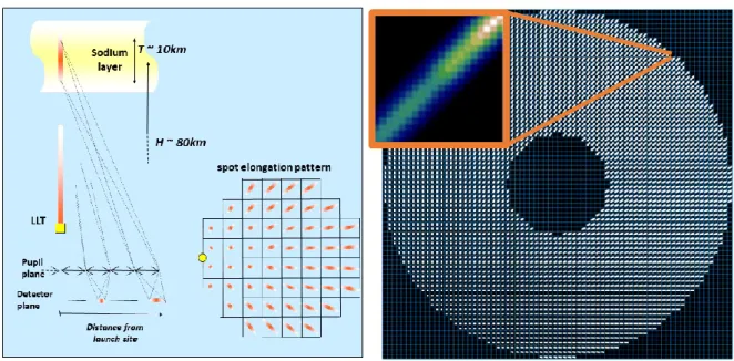
LGSs are needed to maximize the sky coverage offered by AO systems in order to enable observing most targets anywhere on the sky. LGSs provide a higher Signal to Noise Ratio (SNR) than most Natural Guide Star (NGS) but induce some well-known drawbacks such as the Tip/Tilt indetermination, the cone effect and the spot extension in 3D. The laser beam illuminates the Sodium layer located at about 80 to 90 km above the ground. The excited sodium atoms emit light in return. We can therefore consider the patch of illuminated Sodium atoms as a secondary object. This object is extended in the transversal plane due to the size of the laser waist (~ 50 cm) and also along the longitudinal axis as the sodium layer typical width is about 10 km. The Z extension of the 3D object is imaged at the focal plane as an extended spot through a subaperture located at a pupil position that is not collocated with the laser launch telescope. This effect is magnified with a side launch scheme as used at the VLT (AOF at UT4 [3] [4]) and planned for the ELT (see Figure 1). In the ELT case, the worst case corresponds to an elongation ratio of around 24 between the long axis and the short axis of the spot imaged through the furthest subaperture from the laser launch telescope. This means that for this subaperture the photon noise variance is ~ 600 times larger along the large axis. In other words, the small axis component of the

measurements is worth several hundreds of long axis measurements in terms of SNR. Moreover, beyond a degraded SNR, the spot elongation yields a bias on the reconstructed wavefront when the spots are truncated and/or not properly sampled. We will explore these effects in the next sections.

Figure 1: Illustration of LGS spot elongation on a Shack-Hartmann focal plane at the ELT 2.2 Assumed LGS return flux

Figure 2: Statistics of LGS return flux based on VLT/AOF/4LGSF experience – averaged through the year, median conditions, seeing=0.67” Flux levels (colors) in Millions photons/second/m2

To properly evaluate the WFS measurement SNR, one needs to consider a realistic operating point in terms of flux per subaperture per frame. Considering an estimated MAORY throughput of 23% at 589 nm, we expect to get 960 photons per subaperture per frame at 500Hz framerate based on the average return flux observed at the VLT with 4LGSF (see Figure 2 and [2]). The ICD with the telescope is slightly more conservative with 820 photons per subaperture per frame under median conditions while more than 470 photons per subaperture per frame will be collected in 90% of the cases.

We will use the latter flux value to dimension our LGS WFS in order to provide a robust performance, as can be expected from a workhorse instrument.

2.3 One problem, many solutions

Many solutions have already been proposed to deal with the issue of LGS spot elongation and spot truncation. Here is a non-exhaustive list of possible mitigations:

• Laser range gating and dynamic refocusing removing the LGS extension but leading to a loss of useful photons • Custom detector geometry such as the radial CCD combined with LGS central launch for TMT/NFIRAOS • Focal plane shaping: optimized lenslet array and optical shrinkage of the focal plane spots pattern [5] [6] [7] • Advanced centroiding algorithm: correlation, matched filter [8], requiring Sodium profile knowledge • Pupil plane WFS: Pyramid WFS, INGOT [9]

• Shack-Hartmann with many pixels → CMORE [12] [20]

• Reference WFS to deal with propagated bias. For MAORY, we have simulated that such truth sensing loop must be slow (cut-off <0.01 Hz) to avoid hindering the compensation of atmospheric turbulence

In this paper, we will focus on the following mitigation avenues: • Optimized tomographic reconstruction with side launched LGS

• WFS design: Pixel scale/Subaperture FoV as well as an optimized centroiding algorithm to reject RON

In this framework, we will perform a trade-off analysis between sensitivity and linearity, between a good sampling of the PSF, with many pixels and a low propagation of the Read-out noise (RON), with less pixels. This analysis is performed under technological constraints. In particular, the number of pixels is limited to 800x800 per WFS, that is 10x10 pixels for each of the 80x80 subapertures. Our trade-off philosophy is driven by robustness considerations. We will prefer a solution that is less sensitive to a wrong tuning or a change of the environment at the potential cost of a marginal loss of performance. Finally, we will avoid when possible the necessity for calibration or prior knowledge. We will also favor the design cases for which a static tuning is sufficient and no online optimization is needed.

3. THE MAORY CASE

3.1 Main input parameters

In this study, the main AO parameters are in line with the current MAORY baseline case [10]: • 6 LGS WFS @ 45” radius on sky with

o 80x80 subapertures across a diameter of 39 m – lenslet array rotated by 45° to align the subaperture’s diagonal with the worst elongation direction

o 10x10 pixels per subaperture o Read-out noise: 3e- rms • 35 layers Cn2 _{profile with r}

0=0.157m at zenith and L0=25 m

• A tomographic reconstruction based on POLC/MMSE [11]

• The numerical simulations are powered by OCTOPUS/FRIM3D [15] [16] and realistically address the following terms of the error budget:

o Tomographic error o Generalized fitting o Aliasing

o Temporal error

o TT temporal error but no noise and low anisoplanatism: bright TT star, good asterism

3.2 Spot sampling considerations

It is well known that the linear number of pixels per spot full width at half maximum (fwhm) shall be greater than 1 to keep the noise variance under control [10].Indeed, an undersampled spot will give rise to non-linearities and sensitivity to spot size changes (seeing variation especially). In the MAORY case, when investigating large subaperture FoV to reduce spot truncation, the pixel scale becomes so large that we enter the severely undersampled regime. For example, in Figure 3 a FoV of 20” hence a pixel scale of 2” leads to a strong non-linearity of the slope response with an LGS spot of 1.1” fwhm which is typical under good seeing condition. Thus, for such large subaperture FoV cases, under the constraint of 10x10 pixels per subaperture, the LGS fwhm must be increased to keep one pixel per fwhm. This can for example be achieved by defocusing the LGS beam either at the level of the launch telescope or at the level of the WFS lenslet array. The penalty in terms of photon noise is acceptable thanks to the comfortable amount of flux collected at our typical working point as mentioned in section 2.2.

Figure 3: Slope response [Right] When sampling a spot of 1.1” fwhm [Left] with a pixel scale of 2”

Figure 4: [Top] High resolution elongated LGS spot [Bottom] Low resolution LGS spot 3 with 10x10 pixels [Left] FoV=10”, pixel scale=1”, LGS fwhm= 1.1” [Middle] FoV=15”, pixel scale=1.5”, LGS fwhm= 1.5” [Right]

FoV=20”, pixel scale=2”, LGS fwhm= 12”

In the following study , we will consider 3 dimensioning cases: FoV=10, 15 and 20”. For each of them the spot is enlarged so that its fwhm is equal or larger to the pixel scale, respectively 1”, 1.5” and 2” as seen on Figure 4.

3.3 Evaluation of the quasi-static bias by single channel open loop reconstruction

A non-uniform truncation across the pupil plane leads to a bias of the reconstructed wavefront. A simple way to evaluate this bias is to simulate the WFS slopes generated by a flat wavefront, to reconstruct the slopes in the phase space and

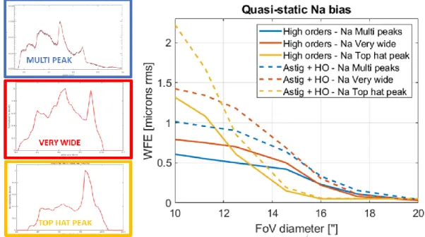
project the bias onto optical modes. We perform this simulation in a pessimistic case that magnifies the phenomenon in order to highlight this effect. Indeed, we perform a phase reconstruction based on a single wavefront sensor measurement, not benefiting from the multiplicity of measurements provided by a MAORY like system, nor from any sort of regularization. Instead, we use a classical Shack-Hartmann with no noise and a classical center of gravity. The sodium profile is centered in terms of Tip/tilt and defocus. Anyway, untruncated spot can only generate bias along Tip/Tilt and defocus. We will not consider these three modes as they are managed by the jitter loop and the Sodium altitude tracking loop or focusing loop. In Figure 5, the generated bias is plotted against FoV for 3 cases of Sodium profile from the most gentle to the most pathological: multi-peak, very wide and top hat with peak at the edge.

As expected, the bias projects strongly along the two astigmatisms. The total bias amplitude is dramatic for a FoV of 10” where the spot truncation is severe. Then, the amplitudes decreases with the FoV and becomes small for a FoV of 20”. This analysis confirms that our cases of interest are well chosen, with a FoV spanning a range from 10” to 20”. It is also worth noting that even with such pessimistic assumptions, the case with a FoV of 20” is almost immune to quasi-static bias.

Figure 5: Bias expressed in WFE (microns rms) as a function of subaperture FoV for 3 different sodium profiles multi-peak (blue), very wide (red) and top hat with peak at the edge (yellow). [Solid lines] high order modes

[Dashed lines] All modes: high order modes and astigmatisms

4. DEALING WITH SPOT ELONGATION WITH TOMOGRAPHIC RECONSTRUCTION

4.1 Side launched LGS

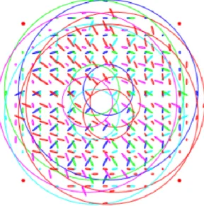
In the previous section we have analyzed the bias generated by the non-uniform spot truncation in the case of a single WFS. However, MAORY is a tomographic AO system and the purpose of implementing multiple WFSs is to sense the 3D turbulence. The WFS asterism geometry is optimized to sample each significant turbulence layer by combining the signals from all WFSs. Some areas of the altitude metapupils are only sampled by one LGS beam while others where the beams overlap are sampled by several WFSs. Figure 6 shows an illustration of one metapupil sampled by four LGS beams whose subapertures’ spot are projected onto the altitude layer. It is interesting to note that the side launch configuration helps create diversity in the measurements from several WFSs. Other outstanding features can be highlighted:

• The redundancy of the metapupil sampling offers in each subaperture several measurements across the small axes of the overlaid spots, hence the signal with highest SNR

• In the non-overlapping areas the spot is least elongated, we are lucky !

Figure 6: Illustration of 4 LGS beam footprints overlap and overlaid spot pattern in an altitude metapupil in the case of side launch scheme

The geometry of the spot elongation is a key parameter to be taken into account in the tomographic reconstructor. We will see in the next section that three tomographic reconstruction model parameters are to be optimized:

• The regularization term: turbulence phase covariance

• The spot geometry across the pupil of each WFS, including the elongation • The model of WFS measurement errors

4.2 Regularization with OCTOPUS/FRIM3D

The complete recipe to deal with spot truncation with a tomographic AO system has been formalized by M. Tallon et al. between 2008 to 2010 ([13][14]). In OCTOPUS/FRIM3D ([15] [16]), the POLC-MMSE reconstructor uses as priors the covariance of the phase and the WFS measurements covariance Cn whose inverse writes as shown in Figure 7 with the

following input parameters:

1. σn the noise variance, uniform across the pupil, in nm rms. σn is computed with roundgaussian spots.

2. β the width of the sodium layer in km that yields an noise term which is non-uniform across the pupil.

3. tG the threshold level used to determine, in each subaperture, whether truncation occurs or not. For each subaperture, the following test is performed.

o When β is smaller than the sigma of a gaussian function whose amplitude is equal to tG at the edge of the field of view, the spot is considered not truncated and the inverse of the measurement covariance writes in its usual form (see Figure 7)

o When β is larger than the sigma of a gaussian function whose amplitude is equal to tG at the edge of the field of view, the spot is considered truncated and the slopes from this subaperture are filtered in order to conserve only the component that does not project on the elongated axis. This corresponds to filtering one of the two eigenvectors from this 2x2 matrix. In this case, the 2x2 covariance block corresponding to this subaperture is modified as shown on Figure 7.

As one can see in Figure 7, playing with tG allows determining whether a subaperture lies in the upper case (not truncated) or the lower case (truncated) where the slopes long axis component gets discarded. It is easy to understand by multiplying the lower 2x2 inverse covariance by the coordinates of the vector β . The result is 0 which shows that the

long axis component has been filtered out. Moreover, it is interesting to highlight that when β is significantly larger than

σ, the upper equation tends towards the lower one. This is what happens when the β prior is set to a value that is

voluntarily too large. This approach is called over-regularization [12]. Its effect is to reduce the weight of the long axis component in the reconstruction, but in this case across the whole pupil plane.

Figure 7: [Left] Elongated spot of coordinates [β1 β2] with short axis of fwhm σ and long axis of fwhm β. [Right] Truncation management by writing the measurement covariance matrix block for each subaperture depending whether or not truncation occurs, according to tG and β.

In our study, over-regularization is not used. We set Beta to a realistic value of 10 km and the threshold value tG is tuned to select the eigenvectors to be discarded.

5. END-TO-END SIMULATIONS

The end-to-end simulations are run with Octopus [15] that simulates the physical model of the atmosphere and the system. The FRIM3D [16] module acts as a real time computer that collects the measurements and generates the deformable mirrors’ commands. The main simulation characteristics are the following:

• Low Tip/Tilt error: bright NGS, good asterism • We deal only with “realistically” elongated spots

• LGS Tip/Tilt and defocus are removed when the focal plane spots are generated

• Bias management: reference slopes with flat wavefront are computed for each Sodium profile

5.1 Initial verification

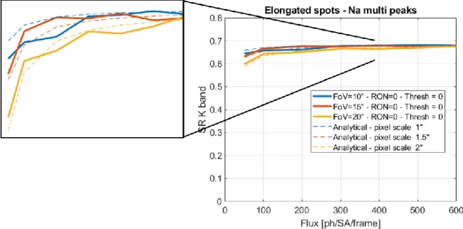
We first check that the simulation behaves as predicted by analytical formulae in a simple case with RON=0. As expected, one can notice that the larger the FoV, the lower the performance at low flux, even though the difference is small (see Figure 8)

5.2 Tuning the regularization without bias

Then, the RON is set to a more realistic value of 3e- rms. This additional noise is managed by tuning the centroiding algorithm. It is based on a windowing approach with a binary window whose shape is following the spot elongation in each subaperture. This window is computed such that it leaves sufficient field of view for all sodium layer profile cases and residual jitter. The window shape must be centro-symmetric to avoid introducing centroid bias. This smart window rejects the noise nicely as one can notice on Figure 9. It obviously corresponds to a particular case of weighted center of gravity. When the tomographic reconstructor is tuned with proper physical parameters (β=10km, σn=80 nm rms) and

when all measurements are kept (no eigenvector is discarded), the largest FoV case performs well. Nevertheless, the 10”FoV case suffers because too many subapertures are truncated.

Figure 8: Verification of the simulated performance against analytical formulae in a simple case with RON=0

Figure 9: On axis performance as a function of flux - no eigen vector is discarded - FoV=10"(blue) FoV=15"(red) FoV=20"(yellow) Reference with no elongation (dash black) Flux level at 90th _{and 50}th _{percentile (dash blue)}

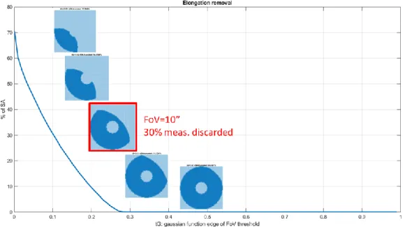
The next step is to tune the parameter tG to maximize the performance in the 10”FoV case. The gaussian function of amplitude tG at the edge of the FoV is narrow when tG is small: many subapertures meet the discard criterion. We then reject the measurement component projecting on the long axis for the subapertures where β is larger than the sigma of the gaussian function. A minimum of one eigenvectors per subaperture is kept. Figure 10 shows that the optimal tG setting for FoV=10”is 0.1, which corresponds to discarding 30% of the elongated components. After tuning the noise prior (σn=160 nm rms) for best performance at low flux, FoV=10” becomes the most sensitive case (Figure 11 blue

diamond curve). However, the performance in the high flux regime is not improved. Tuning the noise prior (σn=50 nm

rms) allows getting the best performance in our flux regime of interest case (Figure 11 blue circle curve). Finally, we obtain very similar performance for the three FoV cases. As expected, the case FoV=20”slightly underperforms because of a higher photon noise.

Figure 10: Tuning of the parameter to maximize the performance in the case fOV=10"

Figure 11: On axis performance as a function of flux - FoV=10"(blue) FoV=10” - 30% discard 160nm rms (blue diamonds) FoV=10” - 30% discard 50nm rms (blue circles) FoV=15"(red) FoV=20"(yellow) Reference with no

elongation (dash black) Flux level at 90th _{and 50}th _{percentile (dash blue)} 5.3 Dealing with bias

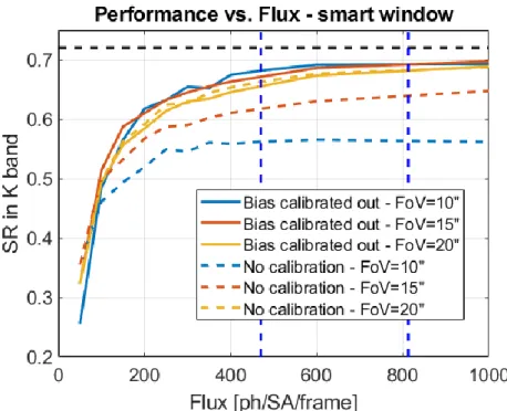
Let us now investigate the impact of uncalibrated bias. Figure 12 shows that the case FoV=20”is insensitive to uncalibrated bias, which makes sense because almost no truncation occurs in this case. Nevertheless, 100 nm rms are

added in the FoV=15”case and 150nm in the FoV=10” case. Thus, for the smaller FoV cases, the bias will need to be calibrated out either by knowing the Sodium profile and using this knowledge in the centroiding process or by means of a natural guide star based truth sensor, managing the bias propagated through the loop. But how about tuning tG in presence of bias ? In this case, it is optimal to discard 65% of the elongated components (Figure 13). Doing this allows to fully recover the performance loss for the cases FoV=10”and 15”. It is interesting to note that the performance does not drop with lower tG values which means that all elongated components could be discarded without performance loss. So, are all these subapertures really necessary ? The question is even more valid because we still have a margin for performance improvement in terms of photon noise. In other words, increasing the level of flux per subaperture above 470 photons per subaperture per frame would improve the strehl ratio.

Figure 12 On axis performance as a function of flux – with calibrated bias: FoV=10"(blue) FoV=15"(red) FoV=20"(yellow) with calibrated bias (dash blue, red and yellow) Reference with no elongation (dash black) Flux

level at 90th _{and 50}th _{percentile (dash blue)}

6. POSSIBLE WFS DIMENSIONING

6.1 Super-resolution

To decrease the number of subapertures without compromising the performance, the concept of WFSing super-resolution has been proposed by S. Oberti [17]. It relies on the fact that the subaperture grids of multiple WFSs are shifted by a fraction of subaperture with respect to one another, which leads to an increased spatial resolution where the grids overlap. This new concept was introduced at AO4ELT5. Meanwhile, its benefit has been successfully simulated for the GMT by Marcos Van Dam (private communication). Super-resolution WFSing has also been empirically proven for the flattening of the NAOMI DM [18]. Finally, its merit has recently been simulated for MAORY, that benefits from the fact that M4 is conjugated at 600 m. This yields a shift of 26% of a subaperture between the WFS lenslet grids projected onto the M4 plane, which provides super-resolution WFSing “for free”. Super-resolution allows reducing aliasing and controlling many more modes than the number of subapertures per individual WFS. Figure 14 shows that going from 80x80 subapertures to 60x60 subapertures induces a very marginal performance loss while gaining a factor 1.8 of additional flux per subaperture. Even dropping to 48x48 subapertures would be acceptable. Indeed, the 75 nm of additional WFE can be fully compensated by the factor 2.8 of increased flux. Finally, such option opens the door to other dimensioning cases. Indeed, less subapertures means more available pixels per subaperture.

Figure 14: Super-resolution concept applied to MAORY [Left] Modal PSD of residual WFE with 80x80 subapertures (red) and 60x60 subapertures (green) [Right] Strehl ratio as a funtion of field radius for 80x80 (red), 60x60 (green), 48x48 (blue) and 40x40 (orange) subapertures

6.2 Design cases

Assuming a desired FoV of 20” where no particular tuning is required to mitigate spot truncation and two detector options (LISA [19] with 800x800 pixels and C-MORE [20] with 1100x1100 pixels), the following design options can be listed:

• LISA – 80x80 SA → FoV = 20” – 10x10 pixels – Pixel scale 2” • LISA – 57x57 SA → FoV = 20” – 14x14 pixels – Pixel scale 1.4” • LISA – 50x50 SA → FoV = 20” – 16x16 pixels – Pixel scale 1.25” • C-MORE – 78x78 SA → FoV = 20” – 14x14 pixels – Pixel scale 1.4” • C-MORE – 60x60 SA → FoV = 20” – 18x18 pixels – Pixel scale 1.1”

7. CONCLUSIONS

• Main trick to keep truncation bias under control: side-launched LGS + proper system model + tomography reconstruction tuning.

• This optimization allows adapting to any dimensioning case that we have studied.

• The larger FoV case (20” diameter) allows avoiding any calibration effort and specific reconstructor tuning. • However, any FoV case is suitable provided the necessary tuning and calibration effort is carried out. • Several hardware solutions:

o Many pixels → CMORE 1100x1100

o Enlarged spot + bigger pixel scale → LISA 800x800 with marginal performance loss o Super-resolution → LISA 800x800

• Next steps:

o Sensitivity study to Sodium profile and Cn2 _profile

o Verification of performance across the FoV

REFERENCES

[1] Diolaiti, E., et al. “MAORY: adaptive optics module for the E-ELT" in [Adaptive Optics Systems V], Proc. SPIE 9909, 99092D (July 2016).

[2] Holzlöhner R., “Lessons learned from 4LGSF”, AO4ELT5 Laser workshop

[3] Kolb, J. et al., “The AOF in operation - challenges and lessons learned” , Proc. AO4ELT6

[4] Oberti, S., Kolb, J., Madec, P.Y., Haguenauer, P., Le Louarn, M., Pettazzi, L., Guesalaga, A., Donaldson, R., Soenke, C., “The AO in AOF”, Proc. SPIE 10703, Adaptive Optics Systems VI, 107031G (10 July 2018) [5] Gendron, E. et al, “Optical solutions for accommodating ELT LGS wave-front sensing to small format

detectors” in [Adaptive Optics Systems V], Proc. SPIE 9909, 99092D (July 2016). [6] Rigaut, F. et al., “SPOOF: Spot Packing Optimisation on Optical Frames", Proc. AO4ELT6

[7] Jahn, Wilfried, “Laser guide star spot shrinkage for affordable wavefront sensors” in [Adaptive Optics Systems V], Proc. SPIE 9909, 99092D (July 2016).

[8] Gilles, L., “Shack-Hartmann wavefront sensing with elongated sodium laser beacons: centroiding versus matched filtering”, Applied optics 45 6568-76 2006

[9] Ragazzoni, R. et al., “Pupil plane wavefront sensing for extended & 3D sources”, Proc. AO4ELT6

[10] Thomas, S., Fusco, T., Tokovinin, A., Nicolle, M., Michau, V., Rousset, G. “Comparison of centroid computation algorithms in a Shack-Hartmann sensor” MNRAS2006 - Monthly Notices of the Royal Astronomical Society, Volume 371, Issue 1, pp. 323-336.

[11] Busoni, L. et al., ”Adaptive optics design status of MAORY, the MCAO system of European ELT”, Proc. AO4ELT6

[12] Gilles, L. et al., “Closed-loop stability and performance analysis of least-squares and minimum-variance control algorithms for multiconjugate adaptive optics”, Applied Optics Vol 44, issue 6, p 993-1002

[13] Fusco, T. et al., “A story of errors and bias: the optimisation of the LGS WFS for HARMONI”, Proc. AO4ELT6

[14] Tallon, M., Tallon-Bosc I., Bechet C. and Thiebaut E., “Wavefront reconstruction for SCAO and GLAO with elongated laser guide stars”, ELT-INS-TRE-09600-0014 FP6 report 2008

[15] Tallon, M. and Tallon-Bosc I., “Wavefront reconstruction with truncated elongated spots on small detectors”, ELT-INS-TRE-09600-0024 FP6 report 2009

[16] Le Louarn, M. et al., “Simulations of Adaptive Optics Systems for the E-ELT”, Proc SPIE 8447, 2012

[17] Tallon, M. et al., “Fractal iterative method for fast atmospheric tomography on extremely large telescopes”, Proc SPIE 7736, 2010

[18] Oberti, S., Guiraud, P., Verinaud, C., Agapito, G., & Plantet, C. “Super-resolution WFSing” forthcoming [19] Woillez, J. et al., “NAOMI: The Adaptive Optics System of the Auxiliary Telescopes of the VLTI”, Astronomy

and astrophysics 2019

[20] Jorden, P. “The Teledyne e2v CIS124 LVSM sensor for large telescopes- design and prototype tests” , Proc. AO4ELT6