Genetic particle filter application to land surface temperature downscaling

HAL Id: hal-03212359

https://hal.archives-ouvertes.fr/hal-03212359

Submitted on 30 Apr 2021

HAL is a multi-disciplinary open access

archive for the deposit and dissemination of

sci-entific research documents, whether they are

pub-lished or not. The documents may come from

teaching and research institutions in France or

abroad, or from public or private research centers.

L’archive ouverte pluridisciplinaire HAL, est

destinée au dépôt et à la diffusion de documents

scientifiques de niveau recherche, publiés ou non,

émanant des établissements d’enseignement et de

recherche français ou étrangers, des laboratoires

publics ou privés.

Rihab Mechri, Catherine Ottlé, Olivier Pannekoucke, Abdelaziz Kallel

To cite this version:

Rihab Mechri, Catherine Ottlé, Olivier Pannekoucke, Abdelaziz Kallel. Genetic particle filter

ap-plication to land surface temperature downscaling. Journal of Geophysical Research: Atmospheres,

American Geophysical Union, 2014, 119 (5), pp.2131-2146. �10.1002/2013JD020354�. �hal-03212359�

RESEARCH ARTICLE

10.1002/2013JD020354

Key Points:

• The use of genetic particle filter to downscale land surface temperature • Good performances of particle

filter downscaling method for a synthetic case

• Application to actual data showed promising performances

Correspondence to:

R. Mechri,

rihab.mechri@lsce.ipsl.fr

Citation:

Mechri, R., C. Ottlé, O. Pannekoucke, and A. Kallel (2014), Genetic par-ticle filter application to land sur-face temperature downscaling,

J. Geophys. Res. Atmos., 119, 2131–2146,

doi:10.1002/2013JD020354.

Received 11 JUN 2013 Accepted 5 FEB 2014

Accepted article online 9 FEB 2014 Published online 6 MAR 2014

Genetic particle filter application to land surface

temperature downscaling

Rihab Mechri1_{, Catherine Ottlé}1_{, Olivier Pannekoucke}2_{, and Abdelaziz Kallel}3

1_{LSCE, UMR 8212, CNRS-CEA, Gif-sur-Yvette, France,}2_{CNRM-GAME, UMR 3589, Météo-France-CNRS, Toulouse, France,} 3_{ENET’Com, ATMS, Cite Ons, Sfax, Tunisia}

Abstract

Thermal infrared data are widely used for surface flux estimation giving the possibility to assess water and energy budgets through land surface temperature (LST). Many applications require both high spatial resolution (HSR) and high temporal resolution (HTR), which are not presently available from space. It is therefore necessary to develop methodologies to use the coarse spatial/high temporal resolutions LST remote-sensing products for a better monitoring of fluxes at appropriate scales. For that purpose, a data assimilation method was developed to downscale LST based on particle filtering. The basic tenet of our approach is to constrain LST dynamics simulated at both HSR and HTR, through the optimization of aggregated temperatures at the coarse observation scale. Thus, a genetic particle filter (GPF) data assimilation scheme was implemented and applied to a land surface model which simulates prior subpixel temperatures. First, the GPF downscaling scheme was tested on pseudoobservations generated in the framework of the study area landscape (Crau-Camargue, France) and climate for the year 2006. The GPF performances were evaluated against observation errors and temporal sampling. Results show that GPF outperforms prior model estimations. Finally, the GPF method was applied on Spinning Enhanced Visible and InfraRed Imager time series and evaluated against HSR data provided by an Advanced Spaceborne Thermal Emission and Reflection Radiometer image acquired on 26 July 2006. The temperatures of seven land cover classes present in the study area were estimated with root-mean-square errors less than 2.4 K which is a very promising result for downscaling LST satellite products.

1. Introduction

Land surface temperature (LST) is one of the most important variable giving access to surface water and energy states. For many applications—agrometeorology, urban climatology, water balance studies, to cite but a few—LST high-resolution monitoring in space and time is required because of its high spatiotempo-ral variability. Nevertheless, despite the growing availability of LST satellite products, the available satellite sensors offer either a high spatial resolution (HSR) or a high temporal one. For instance, the Advanced Space-borne Thermal Emission and Reflection Radiometer (ASTER) has a spatial resolution of 90 m in the thermal infrared (TIR) spectral domain but a bimonthly sampling frequency. The Spinning Enhanced Visible and InfraRed Imager (SEVIRI) radiometer onboard Meteosat Second Generation (MSG) satellite has a sampling frequency of 15 min with a spatial kilometric resolution ranging from 3 km to 5 km. Such coarse spatial resolution (CSR) is not sufficient to monitor surface fluxes and variables on heterogeneous landscapes. Thus, the development of methods to overcome these limitations becomes essential in order to track LST evolution at high spatiotemporal resolutions (HSTR). Different approaches have been so far developed to downscale LST, ranging from linear regression schemes to data assimilation ones; see Zhan et al. [2013] for a review.

The most common approach is based on linear regressions [Kustas et al., 2003; Agam et al., 2007a, 2007b;

Liu and Pu, 2008], which exploit the negative relationship between LST and vegetation density, generally

assessed with the Normalized Difference Vegetation Index (NDVI) (or the vegetation cover fraction fcover),

both increasing with the amount of biomass. In satisfactory soil moisture conditions, the canopy evapo-transpiration is generally higher than the bare soil evaporation (because the root system allows access to deeper water content, combined to the higher surface roughness. For more details, see Olioso et al. [2002];

Douville et al. [2012]). Consequently, vegetated surfaces present generally lower temperatures than

this empirical covariation of LST and NDVI to develop sharpening schemes known as TsHARP (the clas-sical sharpening approach/model) [see Kustas et al., 2003; Agam et al., 2007a, 2007b; Liu and Pu, 2008]. TsHARP approach assumes that LST has a unique relationship to photosynthetically active biomass which can be approached with shortwave reflected radiation (NDVI /f_cover) across a given satellite image scene. To enhance CSR LST, TsHARP uses an inverse linear covariation between NDVI/f_covermaps acquired at HSR and CSR LST maps. This assumption is valid for homogeneous vegetated areas, and good results have been found over rainfed agricultural areas in Agam et al. [2007b]. Yet the validity of LST-NDVI/f_cover rela-tionship remains questionable when working on complex heterogeneous landscapes. Jeganathan et al. [2011] investigated four TsHARP variants over a mixed agricultural landscape in India and concluded that TsHARP is efficient only when locally applied over relatively homogeneous fields and not for regional scales. To address this issue, Inamdar et al. [2008] and Inamdar and French [2009] introduced emissivity data to enhance Geostationary Operational Environmental Satellite LST over the U.S. Southwest region and bet-ter results have been found compared to the classical TsHARP. Merlin et al. [2010] proposed to extend the validity domain of the classical TsHARP by introducing the temperature difference between photosyntheti-cally active and nonphotosynthetiphotosyntheti-cally active vegetation. Statistical results showed improvements in terms of robustness and accuracy, for the disaggregated LST, and better agreement with validation data, com-pared to the classical model. Furthermore, Merlin et al. [2012] introduced a new approach by integrating the main surface parameters involved in the surface energy budget which are open water and soil evapo-rative efficiency in addition to the senescent/green fcover. The method uses a linearized radiative transfer to

relate four satellite products inverted from different shortwave bands at different resolutions to CSR LST. The introduction of open water and soil evaporative efficiency fractions improved the disaggregation results, but the operational application of the method is still not possible because soil evaporative efficiency data are currently not available at fine resolution over large areas. In the case of artificial surfaces, Dominguez et

al. [2011] found that the LST-NDVI relationship is not consistent for urban areas like the city of PuertoRico

and proposed a bivariational model including albedo in addition to NDVI variable in their high-resolution urban thermal sharpener model. This yielded to smaller mean absolute error (MAE) and higher correlation coefficient compared to the classical TsHARP. To extend the validity of sharpening schemes over more com-plex areas and at regional scales a data mining sharpener (DMS) has been introduced by Gao et al. [2012]. The DMS technique builds regression trees between TIR brightness temperatures and shortwave spectral reflectances based on intrinsic characteristics. A comparison between TsHARP and DMS showed that DMS outperforms TsHARP in all the cases (homogeneous areas as well as complex heterogeneous areas). All these semiempirical schemes suppose that the LST relationship to the different observed variables could be reproduced with a linear combination or a polynomial decomposition. However, the relationship between LST and shortwave band signals is much more complicated because of the complexity of the interacting biophysical processes.

Other statistical approaches were proposed to solve the downscaling problem based on data assimila-tion strategies. For example, Ottlé et al. [2008] proposed the inversion of subpixel variables by multilinear regressions constrained by prior temperatures provided by a physical land surface model (LSM). Two spatial stationary assumptions were considered to solve the ill-posed problem. First, the mixed pixels are assumed to be composed of a few fundamental components called end-members. Second, the CSR LST is modeled as a linear combination of end-member temperatures weighted by the proportion of each end-member within the mixed pixel area. The results show rapid decrease of the performances when too much heterogeneous landscapes are considered. Then, Kallel et al. [2013] proposed a more adapted inversion scheme introducing

Markovrandomfieldmodeling to represent LST in space and time. The stationary assumptions were relaxed through sequential inversions of the end-member temperatures by using the maximum a posteriori crite-rion. Compared to the NDVI/f_coverdownscaling approach, better correlations were shown as the physical process interactions are accounted for in the LSM [Kallel et al., 2013].

Even though LSM approaches are more difficult to implement operationally and rely on data and mod-els subject to various sources of uncertainties, they allow to provide prior estimations of the spatial and temporal variability of the surface temperature which can be used to solve the downscaling issue. In this work, we propose a new approach based on an ensemble data assimilation (DA) method. The approach is based on Sequential Monte Carlo filter, also referred to as particle filter (PF) (or particle smoother if observations are taken over a time window), which has been successfully implemented to estimate param-eters or states in nonlinear models [see Doucet et al., 2000; Arulampalam et al., 2002; Del Moral et al., 2010;

Van Leeuwen, 2010; Snyder, 2011]. The idea here is to drive a sharpening algorithm at pixel scale with no

spatial or temporal stationary assumptions, using a dynamic model able to simulate the end-member (or subpixel) temperature variability, and to assimilate the CSR observations. Given the fact that LST is mainly determined by land cover, meteorological forcing and soil moisture conditions, the implemen-tation of an LSM on each type of vegeimplemen-tation (and hydric conditions) present in the CSR pixel should be sufficient for the first step (the end-members are the different land cover classes). In this work, the Suivi de l’Etat Hydrique des Sols (SEtHyS) LSM [Coudert, 2006] was used to simulate the surface temperature of the different end-members and to assimilate the coarse resolution observations. A LSM is a dynamic model rep-resenting the energy and mass transfers governing the soil-vegetation-atmosphere continuum as well as the surface variables in particular soil moisture and surface temperature. The originality of our approach is the use of a DA method to simultaneously downscale CSR data and calibrate the LSM parameters for all the end-member temperatures making up the CSR pixel grid cell. Our paper is organized as follows: the DA approach and its application on a synthetic pixel composed of four end-members is presented in section 2. Section 3 gives the details on the experiment setup and the resulting downscaled temperatures and dis-cusses the performances of the method considering the observation sampling and the errors statistics. The application of our approach on actual data is presented in section 4. A summary and conclusions are given in section 5.

2. Methodology

In the following work, we assume that the subpixel (end-member) temperature variability is mainly attributed to land cover heterogeneity. Then, the objectives are to estimate the respective temperatures of each land cover class inside a mixed pixel composed of fractions of these different vegetation types. This assumption is valid at regional scale (few kilometers size) where the atmospheric forcing can be supposed homogeneous and when flat landscapes are considered. In our case, the prior knowledge of the vegeta-tion classes fracvegeta-tions within the CSR pixel is needed and can be provided by a HSR land cover mapping. The problem can be addressed by constraining a dynamic LSM able to simulate prior subtemperatures and pixel-aggregated temperature given the fractions of each vegetation type, with the assimilation of CSR. The following section presents the DA developments and their implementation in the SEtHyS LSM.

2.1. The Particle Filter

Data assimilation aims to provide the best estimation of the state of a system or its unknown parameters,

x_q, using observations, y_q. The system is assumed to evolve according to a Markov process featured by the transition probabilities p(x_q|x_q−1) and represented by the propagator x_q+1= (x_q). The observations y_qare related to the state xq, thanks to the nonlinear observational operator according to yq= H(xq) + 𝜀oqwhere

𝜀o

qdenotes an error modelized as a random centered Gaussian vector of covariance matrix Rq. The general

estimation Bayesian framework is given by the nonlinear filtering theory [Jazwinski, 1970]. It describes the time evolution of the full probability density function p(x_q) conditioned by the dynamics and the obser-vations. The probability dynamics can be expanded in two steps: a forecast step and an analysis step. The forecast step is obtained from the Chapman-Kolmogorov rule

p(xq|yq−1) = ∫ p(xq|xq−1)p(xq−1|yq−1)dxq−1 (1)

while the analysis step is deduced from the Bayes rule as

p(xq|yq) ∝ p(yq|xq)p(xq|yq−1) (2)

(to within a normalization term). An analytic solution of the distribution evolution can be obtained for lin-ear dynamics and Gaussian distributions, leading to the Kalman filter equations [Kalman, 1960]. However, for practical applications where distributions are not Gaussian and their dynamics not linear, this approach requires additional simplifications where a sampling distribution is considered in place of full distribu-tions. This leads to the ensemble Kalman filter algorithm [Kalman, 1960] for the nonlinear ensemble-based

extension of the Kalman filter, or the particle filter approach [Doucet et al., 2000; Del Moral, 2004] for the discretization of the nonlinear filter. It follows that the density p(x_q) is approximated as the empirical density

p(x_q) ≈ p_N(x_q) = 1 N ∑ k 𝛿xk q (3) where xk

qis an ensemble of N independent identically distributed samples of the law p(xq) and where 𝛿

denotes the Dirac’s distribution located in the sample xk

q. From this discrete point of view, the analysis step is

equivalent to p(xq|yq) ≈ pN(xq|yq) = ∑ k w_qk𝛿xk q (4) where w_qk= p(yq|xqk ) ∑ ip ( y_q|xi q ) (5)

At each analysis step, a new ensemblêxk

qis obtained from the sampling of the distribution pN(xq|yq) so that

p(xq|yq) ≈ 1 N ∑ k 𝛿̂xk q (6)

The forecast step is now written as follows:

p(xq+1) ≈ _N1 ∑ k 𝛿xk q+1 (7) where xk

q+1 = (̂xqk) denotes the ensemble of forecast deduced from the states ̂x k

q. The filter can be

extended into a smoother considering observations over an assimilation window [see Del Moral, 2004; Rémy

et al., 2012]. In this case, we assume the availability of M observations between two analysis times q and q+1:

(ym

q)m=1,…,M. The potential function gmq

( xk q ) = p(ym q|xkq )

, which designs the likelihood function in filtering problems, allows to decide whether a particle xqis killed (with low potential) or kept (with high potential)

and duplicated into several offsprings. The weights can be expressed as follows:

wk m= gm ( xk q ) ∑N j=1gm ( xqj ) (8) Finally, we have Gq(xkq) = M ∏ m=1 gm_q(x_qk) Wk_q= M ∏ m=1 wk_m= G_q(xk q ) ∑N j=1Gq ( xj_q) (9)

2.2. Genetic Selection-Multinomial Resampling

One of the major drawbacks of PF schemes is the degeneracy phenomenon. In fact, after several iterations, all but one particle will have negligible weight. A suitable measure of degeneracy of the PF algorithm is the effective ensemble size N_eff[Bergman, 1999; Arulampalam et al., 2002]. In our case, the estimation of N_effcan be obtained by Neff= [_N ∑ k=1 ( W_qk)2 ]−1 (10) where N is the ensemble size and Wk

qis the normalized weights defined in equation (9). According to the Neff

definition in equation (10), we have Neff ≤ N. Small Neffindicates severe degeneracy. Such problem could

be avoided either by choosing very large ensemble sizes, which is often impractical, or by resampling the particles. A review of particle filter resampling schemes is presented in Arulampalam et al. [2002] and Douc

In our case, we choose to work with the basic genetic particle filter (GPF) with multinomial resampling, which belongs to the genetic algorithm (GA) family. In fact, the particle filtering problem could be studied from a GA perspective if we focus on the selection-resampling step. GA could be defined as a stochas-tic searching algorithm (a function optimizer) ensuing from Darwin’s evolution theory, simulating the well-known survival of the fittest individuals evolution. The fitness of an individual could be presented as the closeness of a chromosome from the optimal solution. Fitter individuals crossbreed and produce better offsprings to improve the whole population fitness. Mutation could also happen during offspring produc-tion. This definition highlighted two main similarities between GA and PF: the first one is the selection of the “best” offsprings according to their closeness to the optimal solution (selection of particles with higher potential G_q), and the second one is the crossover and mutation to produce the new offsprings that pro-mote the whole population (resampling particle from the selected particles distribution). More details on the GPF implementation is available in Uosaki et al. [2004] and Kwok and Zhou [2005].

Once particles are selected, a multinomial resampling [Rémy et al., 2012] is performed to produce the new population from the selected particles (mutation). The multinomial algorithm replicates particles with higher weights, and a noise is added to copied particles. This noise is chosen large enough to differentiate copied particles from seed ones (to allow a better exploration of the solution space) and keep coherent with model uncertainties (to avoid filter collapse when the noise is too large). More details on the genetic selec-tion and multinomial resampling implementaselec-tion of PF algorithm could be found in Kwok and Zhou [2005] and Rémy et al. [2012].

2.3. Downscaling-Calibration Approach

As already mentioned in the introduction, the SEtHyS LSM [Coudert, 2006] has been used to assimilate the coarse observations and to estimate the subpixel temperatures. SEtHyS predicts the surface temperature evolution by solving the hydric and energy budgets at the land surface. It is forced with micrometeorolog-ical parameters such as air temperature and humidity, downwelling shortwave and longwave radiations, irrigation/precipitation, and wind speed. Two sources are used to represent the soil-vegetation-atmosphere system: the soil and the aboveground vegetation. An energy budget is computed for both sources, and con-sequently, both temperatures are determined. A detailed description of the radiative transfer in the solar and thermal infrared domains allows to compute the directional surface reflectances and radiative temper-ature above the canopy [Coudert et al., 2008]. The model has been already used to test LST downscaling approaches in previous studies [Ottlé et al., 2008; Kallel et al., 2013; Guillevic et al., 2012], and particularly on the “Crau-Camargue” agricultural site in southeastern France (43.53◦N, 4.66◦E). The case study chosen for this work consists of a single pixel composed of four end-members equally distributed in order to represent a typical agricultural area. The climate of the study region is Mediterranean, with irregular rainfall, long dry periods in spring and summer, and strong winds. The micrometeorological forcing database for the year 2006 [Courault et al., 2008] was used in our test case. The four end-members composing the CSR pixel are agricultural. During the spring/summer period, which will be used in the assimilation tests, bare soil, prairie, wheat, and rice fields can coexist. In the following, we design by the subscripts “1,” “2,” “3,” and “4” the dom-inant land cover classes “Bare Soil,” “Prairie,” “Wheat,” and “Rice.” Their respective fractions were set equal to 0.25 and assumed constant during the study period. For each of these classes, reference soil and vegeta-tion parameters were assigned and were used to generate reference temperatures over the year 2006. These temperatures will be further considered as reference subpixel (or end-member) temperatures and aggre-gated to generate CSR pseudo-observations that will be used in the assimilation process. A white Gaussian noise𝜀o

qwas added after aggregation to generate noisy observations. The observation error amplitude was

initially set to the standard value of 2 K similarly to Kallel et al. [2013]. The impact of the observation error amplitude on the assimilation performances has been studied in a second step. In our case, the particles represent a set of SEtHyS parameters corresponding to the different classes. More generally, the particle can be represented as follows: x_q=[P1 1,q, … , P1D1_,q, P 2 1,q, … , PD22_,q, P 3 1,q, … , P3D3_,q, P 4 1,q, … , P4D4_,q ] , (11) where(Di₎

i∈[1∶4]refers to the number of selected parameters for the land cover class i. The model, as

rep-resented in the subsection 2.1, is the particle propagator. Given that particles (SEtHyS parameters) remain static during an assimilation window, is, in our case, the identity function to which a white Gaussian noise with a standard deviation (SD) equal to𝜎_𝛽= 0.1 is added after every resampling step: xk

q+1= x k

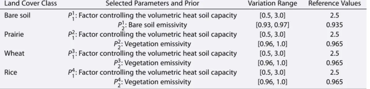
Table 1. SEtHyS Parameters Used for the Calibration

Land Cover Class Selected Parameters and Prior Variation Range Reference Values Bare soil P1

1: Factor controlling the volumetric heat soil capacity [0.5, 3.0] 2.5 P1

2: Bare soil emissivity [0.93, 0.97] 0.935

Prairie P2₁: Factor controlling the volumetric heat soil capacity [0.5, 3.0] 2.5

P2

2: Vegetation emissivity [0.96, 1.0] 0.965

Wheat P3

1: Factor controlling the volumetric heat soil capacity [0.5, 3.0] 2.5 P3₂: Vegetation emissivity [0.96, 1.0] 0.965

Rice P4

1: Factor controlling the volumetric heat soil capacity [0.5, 3.0] 2.5 P4

2: Vegetation emissivity [0.96, 1.0] 0.965

where k refers to the kth particle (k ∈ [1, … , N]), 𝜉q = 

( 0, 𝛽q

)

and𝛽q = 𝜎𝛽2× I. Indeed, the

nonlinear-ity of land surface processes and the rapid changes of boundary conditions like precipitation or irrigation events and various agricultural practices can lead to rapid changes in surface states and parameter values and impact the estimation of subtemperatures. Such a problem could be overcome with the resampling step. In fact, resampling particles allows to explore globally the parameter space and to find optimal tem-peratures far from the local prior values without being drawn in false directions. A previous temperature sensitivity analysis based on a screening approach [Frey and Patil, 2002] permitted the selection of the parameters to calibrate. The results show that on the study period, two parameters for each class have larger sensitivities. A detailed list of these parameters is available in Table 1. Once the parameters are defined, a first-guess particles ensemble is generated from N random samples of the parameter space (N random draws from a uniform distribution). Every particle leads to a quadruplet of subpixel prior temperatures [ Tk 1, T k 2, T k 3, T k 4 ]

k∈[1,…,N], as output of SEtHyS model (the subpixel temperatures are completely determined

once the parameters fixed). Then, these N subpixel temperatures are aggregated and compared to the syn-thetic observations using the GPF. Then, a weight is attributed to each particle according to the discrepancy between the observed temperature Toand the simulated aggregated temperatures Ts. At the end of the

analysis step, the mean of the subpixel temperatures corresponding to the selected particles represents the solution of the downscaling problem. The kept particles are resampled to create the new set of calibrated SEtHyS parameters. The definition of the observation operator is described by equation (12), and the distance between the observation “Y_q” and a particle “xk

q” is given by equation (13). (xk q ) = ⎡ ⎢ ⎢ ⎢ ⎣ ∑ i∈[1∶4]𝛼i𝜖i{ ( xk q ) }4 ∑ i∈[1∶4]𝛼i𝜖i ⎤ ⎥ ⎥ ⎥ ⎦ 1 4 = [ ∑ i∈[1∶4]𝛼i𝜖iTi,q4 ∑ i∈[1∶4]𝛼i𝜖i ]1 4 (12) ||(xk q ) − Yq|| = √ √ √ √ √ √ √ √ √ ⎡ ⎢ ⎢ ⎣ (_∑4 i=1𝛼i𝜖i ( Tk q,i )4 ∑4 i=1𝛼i𝜖i )1 4 − To,q ⎤ ⎥ ⎥ ⎦ 2 𝜎2 O (13) where designs SEtHyS model, superscripts k and q refer, respectively, to the kth particle and the qth time window,𝜖iis the surface emissivity of the ith class, and𝛼iis the corresponding cover fraction.

The charts of Figure 1 give an overview of the downscaling-calibration process. The first chart (Figure 1a) presents in details the observation operator H, and the second one (Figure 1b) presents the downscaling-calibration loop.

3. Results and Discussion

In this section, we present the results obtained by the application of the particle filter on the synthetic pixel previously described in section 2. The performance of the downscaling approach is discussed in terms of efficiency, in relation with the amplitude of the observation errors and the observation sampling.

GPF

(a)

(b)

Figure 1. (a) The different parts of the H operator diagram. The subscriptsF,D, andNdesign, respectively, the number of classes present in the CSR pixel, the number of parameters to calibrate for each class, and the number of particles. (Tclass_i)_{i∈{1,…,N}}present the N CSR temperatures corresponding to the N particles (SEtHyS outputs). (b) An overview of the different steps inside the GPF downscaling-calibration process. The subscriptK, refers to the number of kept particles after the genetic selection.

3.1. Experimental Settings

For clarity, in the following, we will omit the time subscript ”q”. For each land cover class, the synthetic ref-erence temperatures and the pseudo-observations were generated on a 124 day period, starting from 28 April 2006 at a 20 min time step. Observations are assumed unbiased. The standard deviation (SD) of the observation error𝜎_Owas set to a value of 2 K (to be comparable to the previous work of Kallel et al. [2013]). The particle ensemble size was set to N= 200 after a series of tests to avoid collapse [Rémy et al., 2012]. At the beginning of the assimilation period, wheat, rice, prairie, and bare soil coexist. The wheat class is, how-ever, in a senescent phenological phase and was harvested on 20 May. Thus, the whole assimilation period was divided in two periods. In the first one,(P1), from 28 April to 20 May, the CSR pixel contains four dis-tinct classes and in the second one,(P2), from 21 May to 29 August, only three classes remain in the CSR pixel (bare soil, prairie, and rice). The micrometeorological forcing data were independently acquired for the three vegetation classes and assumed equal for bare soil and wheat, because the hydric states of these two land cover classes are very close. Indeed, unlike prairie and rice classes which are irrigated, wheat and bare soil are very dry. Leaf area index (LAI), vegetation height, and soil texture were prescribed according to field measurements.

3.2. Downscaling Results and Impact of Observation Error Amplitude

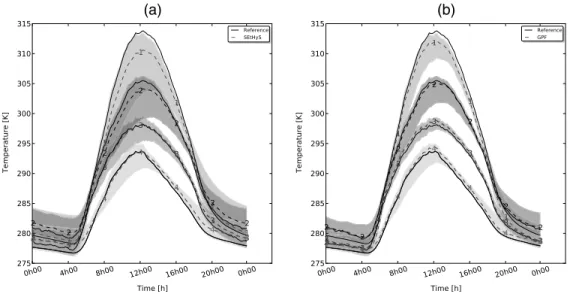
In all the synthetic experiments, the assimilation is performed continuously with an assimilation window of 1 day with a maximum number of 72 observations∕assimilation window. Only the results obtained for period(P1) are shown here. Actually, (P1) is the period when the four classes present the most different properties since wheat was harvested at the beginning of period(P2) and comes down as bare soil. The GPF performances are evaluated by comparing prior and posterior downscaling results over the assimi-lation period. From the start of the assimiassimi-lation process, a significant reduction of the ensemble variance was observed. Figure 2 shows the prior (Figure 2a) and posterior (Figure 2b) downscaling results for the 6th assimilation window. The assimilation of CSR observations has significantly improved the downscaling results. The downscaled temperatures of the four classes are closer to the reference values (RMSE_prior= 1.2K, RMSE_posterior = 0.3K). Figure 3 presents the mean average diurnal cycle of surface temperature over the period (P1). Comparing the prior (Figure 3a) and posterior (Figure 3b) diurnal cycles, the spread of solutions is largely reduced (40% reduction) and the classes are properly separated. However, the improvement is less significant than for the 6th time window. In fact, the filter performances are fairly sensitive to meteo-rological conditions such as windy or nonlimited soil moisture conditions and to observation noise. Since the observations are noised randomly, some days will be more or less noisy than others. Indeed, mete-orological changes occurring along the assimilation period such as strong winds characterizing the rice

Figure 2. Downscaling temperatures for Day 6 (3 May 2006). (a) The prior downscaled temperatures compared to the reference temperatures. (b) The downscaled temperatures after assimilating CSR observations. The line markers 1, 2, 3, and 4 correspond to bare soil, prairie, wheat, and rice classes, respectively. The continuous lines correspond to the reference subpixel temperatures.

forcing data and irrigation practices of the prairie class lead to a decrease of the simulated temperatures (two irrigations at day of year (DOY) 122 and DOY 137 and two precipitation events at DOY 128 and DOY 133 occurred during period(P1)). In these cases, the subtemperatures tend toward the air temperature (Ti≈ Tair,

i∈ {2, 4}) assumed to be exact. The prior error tends therefore to zero, and the assimilation of CSR

observa-tions does not really improve the downscaling results. To illustrate the contribution of the CSR observaobserva-tions, the efficiency rate (see equation (14)) has been calculated.

i[%] = ( 1−RMSE k posterior RMSEi_prior ) i∈[1∶4] × 100 (14)

The mean of the efficiency rates on the first period (P1) are shown in the second column of Table 2. In fact, the more efficient the GPF, the closestii∈[0∶4]to 100%. The results averaged over 100 realizations on the

Figure 3. Downscaling temperatures for the period (P1). (a) The prior downscaled temperatures compared to the refer-ence temperatures. (b) The downscaled temperatures after assimilating CSR observations. The line markers 1, 2, 3, and 4 correspond to bare soil, prairie, wheat, and rice classes, respectively. The continuous lines correspond to the reference subpixel temperatures.

Table 2. Efficiency Rates for Different Amplitudes of the Observation Error SD𝜎_O

Land Cover Class k

𝜎O=0.5 K  k 𝜎O=2.0 K  k 𝜎O=4.0 K Bare Soil 54% 56% 53% Prairie 33% 30% 26% Wheat 60% 59% 54% Rice 48% 46% 43%

period (P1) showed that the downscaling is more efficient for the wheat and the bare soil land cover classes. The respective efficiency rates are 59% and 56%. Lower rates were found for rice (46%) and prairie (30%). This skill reduction is explained by the hydric conditions of these two classes. Indeed, rice and prairie are well irrigated and evapotranspiration is close to potential rates. Therefore, their respective temperatures are close to the air temperature and the prior model error is lower compared to bare soil and wheat classes. The contribution of the observations is then lower. These synthetic experiments have been carried out for 2 other values of the observation error (SD), 0.5 K and 4 K, in order to evaluate the impact of the observation error amplitude on GPF-downscaling method performances (respectively, columns 1 and 3of Table 2). Assimilating CSR observations has significantly improved the estimation of the subpixel tem-peratures for the different classes (i ≥ 25%, ∀i ∈ [1 ∶ 4]). The results show also that GPF performances

decrease with the amplitude of SD as expected (the larger the SD value, the less confidence we have in the observations).

3.3. Impact of Observation Sampling on GPF Performances

The effect of observation sampling on GPF skills was investigated and the contribution of nighttime obser-vations as well. The observation error standard deviation was still set to 2 K, and the obserobser-vations were provided for different periods of the day. Four scenarios have been tested. In the first three scenarios, the time step of the observations was set to 20 min, but the day time observation period was different. The dif-ferent scenarios are described below: (i) Scenario 1: all the observations are available (i.e., 72 observations per day), (ii) Scenario 2: the observation window is daytime only ([10:00 → 18:00], i.e., 25 observations), (iii) Scenario 3: the observation window is 4 h around noon ([10:00 → 14:00], i.e., 13 observations), and (iv) Sce-nario 4: only one observation is available at noon (12:00). The objective of these experiments is to assess the impact of the observation time period on the performances of the GPF-downscaling approach and the con-tribution of nighttime observations (before 10:00 and after 18:00) on the downscaling results. A number of 100realizations for each of these scenarios were performed, and the efficiency rates were calculated. The results illustrated in Table 3 were obtained by averaging the efficiency rates over the 20 day assimilation win-dow of the period (P1) and 100 realizations. At first sight, a slight decrease of GPF performances is noticed when the number of observations decreases. In fact, observations retrieved before 10:00 and after 14:00 do not really improve downscaling results (nonsignificant differences between the efficiency rates which are less than 10%). Thus, we can conclude that the contribution of nighttime observations is much lower than daytime ones and that the most important observations are those acquired during the daytime period when the surface temperature deviation from the air temperature is the largest (see Figures 2 and 3). In Scenario 4, despite the few number of observations (only one observation per day), the efficiency rates are still positive and above 20%. Such result is very interesting and proves the added value of the GPF even with a limited number of observations. To better assess this point and the impact of the observation time, vari-ous scenarios similar to Scenario 4 have been performed varying the observation time during the daytime period of the assimilation window (since nighttime observation contribution is not important, only obser-vations between 6 A.M. and 6 P.M. were considered). Table 4 presents the different scenarios performed and their respective efficiency rates (averaged over 100 realizations). Results show that for all land cover types the best efficiency rates are obtained when the observation is available in the morning (maximum efficiency rates are at 10 A.M. and 12 A.M.). However, for wet classes such as prairie and rice, the efficiency rates are less sensitive to the observation time (nearly the same value for all the observation times). This result confirms our first conclusion about the contribution of noontime observations in the case of a single observation

Table 3. Efficiency Rates for Different Observation Times/Frequencies Land Cover Class Scenario 1 Scenario 2 Scenario 3 Scenario 4

Bare Soil 56% 55% 54% 39%

Prairie 30% 26% 26% 20%

Wheat 59% 56% 55% 44%

Table 4. Scenario 4: Efficiency Rates for Different Observation Times

Observation Time 6 A.M. 8 A.M. 10 A.M. 12 A.M. 2 P.M. 4 P.M. 6 P.M.

1 33% 36% 40% 39% 36% 33% 33%

2 18% 20% 21% 20% 19% 18% 18%

3 39% 41% 44% 44% 41% 39% 39%

4 31% 32% 34% 34% 31% 30% 31%

availability. Finally, we can draw that the most valuable observations are noontime observations and the best efficiency rates are obtained when more observations are considered over the assimilation window. 3.4. Rank Histogram

To assess GPF performances for downscaling CSR LSTs, rank histograms have been calculated over the whole period (P1). In fact, rank histograms, also known as “Talagrand” diagrams, are interesting tools to evaluate ensemble methods forecasts/solutions by determining their reliability and diagnosing errors in mean and spread. Rank histograms are generated by repeatedly tallying the rank of the verification variable (observa-tions) relatively to ensemble members values sorted in increasing order. In other words, they are a measure of the statistical indistinguishability of an observation from the predicted ensemble values assuming that they are independent realizations of a same predicted distribution function. The flatness of the rank his-togram implies that observations fall with equal probability in each of the different intervals defined by the ensemble prediction values. Thus, the flatness is a measure of the reliability of the prediction system. More details on the implementation of the rank histogram are available in Anderson [1996], Talagrand et al. [1997], and Hamill [1997, 2001]. In our case, the reference CSR rank histogram has been drawn from 1000 repetitions of the Scenario 1 (see section 3.3). A bias of 0.25 K has been considered to get a more realistic observation error representation. The reference temperatures are the same than for Scenario 1. The assim-ilation period is (P1), the ensemble size is N = 200, and the observation frequency is 20 min. After the selection step, the number of selected temperatures is generally less than N= 200. A white Gaussian noise with a SD equal to 0.1 K has been added to copied particle temperatures to be able to draw the reference rank histogram. Figure 4 presents the true rank histogram which shows a slight U shape with a shallow infla-tion located at the low ranks. The U shape reflects that the soluinfla-tion ensemble spread is not large enough to include all reference temperatures. Thus, the probability that reference temperatures falls out the solution interval is large. When comparing the extreme ranks, we notice that rankN_{frequency is greater than rank}0

one (freq(N) = 2.9% > freq(0) = 1.8%). This means that reference temperatures tend to be greater than the maximum selected temperatures. Such behavior was expected since reference temperatures are generated using parameter values that are very close to parameter ranges maximum values. The presence of the shal-low inflation in the histogram is the result of the bias prescribed in the observations as confirmed in a similar experience with no biased observations (not shown here). This interpretation was also found in Hamil’s

Figure 4. Reference LST rank histogram.

[2001] and Wilks’s [2006] works, who noted that the deviation from flatness of a rank histogram can be interpreted as ensemble overdispersion/underdispersion and/or unconditional biases in fore-cast/observations. We should also note that the miss-flatness in the histogram is not huge when comparing the probabilities of the extreme ranks 0 and N to the other ranks (the misfit is less than 3%). Such result confirms that GPF-downscaling solutions are quite reliable even when biased CSR observations are considered. Furthermore, it is true that the flatness of rank histogram tells about ensemble consistency; however, the converse is not true in all the cases [see

Figure 5. The 90 m_×90 m land cover map of the Crau-Camargue area with seven classes.

4. Application of GPF on Actual Data

In this section, the GPF approach is evaluated against actual data acquired over the Crau-Camargue region in southeastern France. An ASTER image was acquired during period (P2) on 26 July at 10:47 A.M. Two ASTER products were generated: the land cover map with 15 m× 15 m spatial resolution in the visible band and the LST map with a 90 m× 90 m spatial resolution in the thermal band. The land cover map has been aggre-gated to the LST map resolution. The initial land cover map classification provided by Courault et al. [2008] separates 12 classes. It has been simplified to get a seven class land cover map by combining some classes with similar soil and vegetation properties (i.e., forest and orchards, salt marches and wetlands, etc.). The

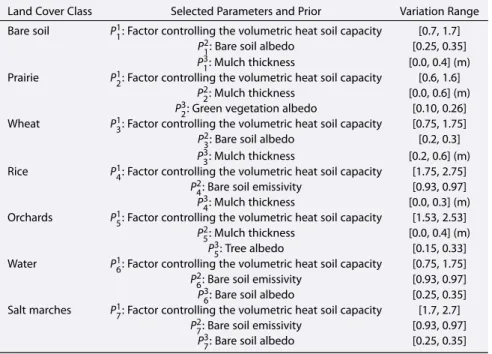
Table 5. SEtHyS Parameters Used for the Calibration: Actual Data Case

Land Cover Class Selected Parameters and Prior Variation Range Bare soil P1

1: Factor controlling the volumetric heat soil capacity [0.7, 1.7] P2

1: Bare soil albedo [0.25, 0.35] P3

1: Mulch thickness [0.0, 0.4] (m)

Prairie P1₂: Factor controlling the volumetric heat soil capacity [0.6, 1.6]

P2

2: Mulch thickness [0.0, 0.6] (m) P3

2: Green vegetation albedo [0.10, 0.26]

Wheat P1₃: Factor controlling the volumetric heat soil capacity [0.75, 1.75]

P2

3: Bare soil albedo [0.2, 0.3] P3

3: Mulch thickness [0.2, 0.6] (m)

Rice P1₄: Factor controlling the volumetric heat soil capacity [1.75, 2.75]

P2

4: Bare soil emissivity [0.93, 0.97] P3

4: Mulch thickness [0.0, 0.3] (m)

Orchards P1₅: Factor controlling the volumetric heat soil capacity [1.53, 2.53]

P2

5: Mulch thickness [0.0, 0.4] (m) P₅3: Tree albedo [0.15, 0.33] Water P1₆: Factor controlling the volumetric heat soil capacity [0.75, 1.75]

P2

6: Bare soil emissivity [0.93, 0.97] P3₆: Bare soil albedo [0.25, 0.35] Salt marches P1

7: Factor controlling the volumetric heat soil capacity [1.7, 2.7] P2₇: Bare soil emissivity [0.93, 0.97]

P3₇: Bare soil albedo [0.25, 0.35]

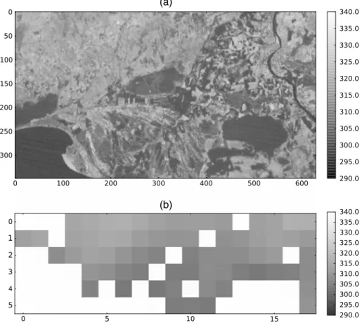
final classes distinguish water, bare soil, wheat, prairie, rice, orchards, and salt marches. Figure 5 presents the new 90 m× 90 m land cover map. CSR LST time series from SEVIRI were also available for the same date over the study area with spatial and temporal resolutions equal to 3 km× 5 km and 15 min, respectively. The SEVIRI LST time series will be used as CSR observations and the ASTER LST as “reference” (“ground truth”) to validate the GPF approach. Since ASTER and SEVIRI sensors have different Earth projection systems (cylin-drical coordinate system universal transverse Mercator for ASTER and nominal geostationary projection for SEVIRI), image coregistration was performed, the ASTER image taken as reference. The two LST products have also been intercalibrated using the Random Sample Concensus (RANSAC) process (more details on this process are available in Kallel et al. [2013] and Fischler and Bolles [1981]). After RANSAC calibration, several SEVIRI pixels, which are not aligned with the best linear regression line (calculated in the RANSAC process), have been removed. Figure 6 presents both ASTER and recalibrated SEVIRI images acquired at about the same time (2 min delay between ASTER and SEVIRI). The comparison of the aggregated ASTER image and the calibrated SEVIRI one showed no bias and better correlation (before correction, bias=−3.02 K, after cor-rection, bias= 0 K, r2_{= 0.86) and the RMS difference (RMSD) between both images is equal to 1.56 K. This}

value of RMSD will be used as the SD of the observation error. The ensemble size was set to N= 200. New

Figure 8. Temperature differences between ASTER and downscaled MSG-SEVIRI LST map.

parameters ranges have been defined for the different classes ensuing from a variance-based sensitiv-ity analysis [Marzban, 2013] performed for the seven classes and using the actual forcing data of the Crau-Camargue region. The micrometeorological and vegetation forcing data have been provided for the different classes according to ground truth measurements. A full description of the selected parameters for the different classes and their boundary values is given in Table 5. Three parameters per class were selected, and their respective variation intervals have been adjusted for the different land cover types according to prior knowledge of the soil characteristics of the case study region. The same variation ranges have been considered for the different classes (mean value±50%). The albedo mean values of the differ-ent end-members have been adjusted according to FORMOSAT albedo products available on the region for the same year [Courault et al., 2008]. The LAI values have been estimated from 90 m resolution NDVI ASTER data for the same day (26 July 2006) following Bsaibes et al. [2009]. Prior end-member tempera-tures (SEtHyS subtemperatempera-tures) have been estimated from 1000 parameter sets. The GPF-downscaling method was applied independently over the different CSR SEVIRI pixels remaining after RANSAC calibration. The assimilation window corresponds to DOY 207 (26 July 2006). Only observations between 06:00 A.M. and 12:00 A.M. were considered because the SEVIRI time series were affected by clouds after 12 A.M. Figures 7 and 8 present, respectively, the downscaled SEVIRI LST image and the absolute difference (AD) map between ASTER LST image and the resulting downscaled image. The results show that more than 50% of the pixels present AD values less than 2 K (dominant dark gray color). The global RMSE, MAE, and Bias between the downscaled SEVIRI image and the ASTER image as well as between the SEtHyS prior estimate image and the ASTER image are presented in Table 6. The results show that the prior RMSE, cal-culated over the remaining CSR SEVIRI pixels, is greater than the GPF one (3 K compared to 2.4 K). The GPF correction may appear not very important compared to other works using the same actual data: in

Kallel et al. [2013], the reduction is about 1.5 K but this result is still promising because the GPF

permit-ted to reduce the prior error with only one run over the DOY 207 assimilation window. We should also note the interesting reduction of the MAE (0.4 K) and of the bias (1.5 K). Table 7 presents for each, land cover type the mean temperatures and their SD for ASTER, SEtHyS, and GPF high-resolution images as well as the RMSE, the MAE, and the bias of the downscaled images compared to the ASTER reference. The results show that for all the classes (except bare soil and wheat), the GPF RMSE are less or equal to the prior ones. The best results are obtained for the prairie and rice classes for which all the statistics were improved. The RMSE have been strongly reduced (from 3.6 K to 1.3 K for prairie and from 6.1 K

Table 6. Global RMSE, MAE, and Bias for the GPF Downscaled SEVIRI and SEtHyS (Prior) Estimated Image Compared to ASTER Image

SEtHyS Results GPF Results RMSE (K) 3.0 2.4 MAE (K) 2.3 1.9 Bias (K) 1.9 ₋0.5

to 1.8 K for rice) as well as the MAE (reduction of 2.4 K for prairie and of 4.4 K for rice) and the biases (reduction of 3.4 K for prairie and of 5.2 K for rice). The statistics have been also slightly improved for salt marches and orchards and remain unchanged for the water class. On the opposite, the results are worse for the bare soil and the wheat classes, whatever the statistical indices. The posterior RMSE, MAE, and biases are larger than the prior ones. This is explained considering that these two classes

Table 7. Reference Data and Downscaling Results for the Different End-Members

Water Bare Soil Prairie Wheat Rice Orchards Salt Marches ASTER LST(◦C) 30.5±2.6 50.2±2.8 36.7±0.4 45.5±2.3 32.7±1.8 40.9±1.5 36.2±2.8 SEtHyS LST₍◦C₎ 33.3_±0.5 50.5_±2.8 40.2_±2.1 47.0_±2.6 38.6_±1.0 42.2_±1.1 37.5_±1.2 GPF LST₍◦C₎ 33.3_±0.2 51.3_±1.5 36.6_±1.2 43.7_±1.9 34.1_±1.9 40.1_±1.1 37.2_±0.6 SEtHyS RMSE (K) 2.2 1.7 3.6 2.1 6.1 1.8 2.1 GPF RMSE (K) 2.2 2.4 1.3 3.1 1.8 1.8 1.8 SEtHyS MAE (K) 1.8 1.4 3.5 1.7 5.9 1.4 1.8 GPF MAE (K) 1.8 2.0 1.1 2.6 1.5 1.5 1.5 SEtHyS bias (K) 1.7 0.2 3.5 1.4 5.9 1.3 1.3 GPF bias (K) 1.8 1.0 −0.1 −1.9 0.7 −0.9 0.5 were the one presenting the lowest prior errors, comparable to the observation error (prescribed to 1.56 K as already noted). In this case, a single analysis step is not enough to constrain the model parameters and more particles are needed to better sample the parameter space in order to obtain errors less or equal than the prior errors. However, these preliminary results are quite satisfactory and demonstrate the potentialities of the GPF approach for downscaling surface temperatures. Compared to current semiempirical approaches, the GPF methodology requires supplementary meteorological data to force the LSM and larger computing resources. However, GPF-downscaling approach allows to monitor dynamically the subtemperatures. Con-cerning computing requirements, the downscaling of a MSG pixel containing seven classes requires 3.51 s of processing time on personal computer. For our MSG image of 68 pixels (remaining after RANSAC from an initial 108 pixel image), 1 min and 2 s is the processing time needed for a sequential implementation of the downscaling algorithm (a loop over the different pixels of the MSG image). A parallel implementation of the GPF-downscaling algorithm could be easily realized and will reduce significantly the processing time. Such requirements allow to envisage operational applications at regional scale.

5. Conclusions

This study investigated the downscaling of land surface temperature through a data assimilation system based on particle filtering. The method uses a dynamic LSM (SEtHyS) able to simulate prior estimations of the temperature time evolution and the spatial variability inside the observed pixel. The subpixel variability accounts for land cover, soil, and atmospheric forcing characteristics, and the pixel is represented by frac-tions of different vegetation classes. The GPF assimilation technique consists of generating an ensemble of candidate solutions for the subpixel temperatures and selecting the ones which minimize the discrepancy between prior aggregated temperatures and the observations at pixel scale and over an assimilation period. The mean of the selected temperatures at the end of the assimilation period is kept as the solution of the downscaled temperatures. In our study, a synthetic pixel composed of four different classes was studied and the assimilation of pseudo-observations was performed on a 124 day period. The particle resampling and selection processes were performed using a daily time window. The results show that the GPF is suitable for LST downscaling because of its easy implementation and its adaptive capability. Indeed, the nonlinear-ity of land surface processes and the rapid changes of boundary conditions, like precipitation or irrigation events and various agricultural practices, can lead to rapid changes in surface states and parameter val-ues. The particle resampling step allows a fuller exploration of the parameter space and to find the optimal temperatures far from the local prior values. Therefore, crucial steps like rainfall events or vegetation phe-nological changes can be overcome without getting trapped in local minima. In our synthetic experiments, the LSM was implemented on four classes of vegetation equally represented, forced with their respective atmospheric and surface conditions provided at smaller scale than the observations. These conditions were prescribed and assumed perfectly known, but uncertainties in these data could be introduced further. In our synthetic experiments, we have tested the assimilation of observations as they could be provided by various space instruments onboard polar or geostationary platforms. As a first step, the observation error statistics were assumed to be unbiased, Gaussian and additive (no time or spatial correlations). The results show that the assimilation improved the estimation of the temperature of the four different land cover classes in all the cases and that the improvement varies with the observation time and with the boundary conditions. The influence of the assimilation is minor when background model errors are the smallest, i.e., when the prior subtemperatures are close to the air temperature (assumed certain), in windy or in nonlim-ited soil moisture conditions. In such cases, the assimilation of noisy observations could even degrade the

downscaling results. The contribution of nighttime observations, in our synthetic case, appears also not sig-nificant, the observations around noon being the most valuable. This is also explained by the lower first guess errors at night compared to daily values. The assimilation methodology was also tested at larger scale on actual data acquired in the framework of the Crau-Camargue experimental database which collects ther-mal infrared data acquired at different scales. The work was performed for 1 day for which SEVIRI LST time series at 15 min frequency and one ASTER image were available. The results show that the subpixel tem-peratures may be estimated with a root-mean-square error lower than 2.4 K after only a single assimilation period of half a day, compared to prior errors reaching for some classes 6 K. These preliminary results prove that GPF is a promising approach for land surface temperature downscaling even if more work is required to better account for land cover map uncertainties as well as observations and model error correlations. The assimilation of multiple instrument (and consequently, multiresolution) data could be also a promising research axis to optimally exploit the irregular observations provided by the existing instruments.

References

Agam, N., W. P. Kustas, M. C. Anderson, F. Li, and P. D. Colaizzi (2007a), Utility of thermal sharpening over Texas high plains irrigated agricultural fields, J. Geophys. Res., 112, D19110, doi:10.1029/2007JD008407.

Agam, N., W. P. Kustas, M. C. Anderson, F. Li, and C. M. Neale (2007b), A vegetation index based technique for spatial sharpening of thermal imagery, Remote Sens. Environ., 107(4), 545–558, doi:10.1016/j.rse.2006.10.006.

Anderson, J. L. (1996), A method for producing and evaluating probabilistic forecasts from ensemble model integrations, J. Clim., 9(7), 1518–1530, doi:10.1175/1520-0442(1996)009<1518:AMFPAE>2.0.CO;2.

Arulampalam, M., S. Maskell, N. Gordon, and T. Clapp (2002), A tutorial on particle filters for online nonlinear/non-Gaussian Bayesian tracking, IEEE Trans. Signal Process., 50(2), 174–188, doi:10.1109/78.978374.

Bergman, N. (1999), Recursive Bayesian estimation: Navigation and tracking applications, PhD dissertation, Linkping Univ., Linkping, Sweden.

Bsaibes, A., et al. (2009), Albedo and LAI estimates from FORMOSAT-2 data for crop monitoring, Remote Sens. Environ., 113(4), 716–729, doi:10.1016/j.rse.2008.11.014.

Coudert, B. (2006), Apport des mesures de température de surface par télédetcetion infrarouge thermisue pour la modélisation des échanges d’énergie et d’eau à l’interface sol végétation atmosphère, PhD thesis.

Coudert, B., C. Ottlé, and X. Briottet (2008), Monitoring land surface processes with thermal infrared data: Calibration of SVAT parameters based on the optimisation of diurnal surface temperature cycling features, Remote Sens. Environ., 112(3), 872–887, doi:10.1016/j.rse.2007.06.024.

Courault, D., A. Bsaibes, E. Kpemlie, R. Hadria, O. Hagolle, O. Marloie, J.-F. Hanocq, A. Olioso, N. Bertrand, and V. Desfonds (2008), Assessing the potentialities of FORMOSAT-2 data for water and crop monitoring at small regional scale in South-Eastern France, Sensors, 8(5), 3460–3481, doi:10.3390/s8053460.

Del Moral, P. (2004), Feynman-Kac Formulae: Genealogical and Interacting Particle Systems With Applications, Probability and Its Applications, Springer, New York.

Del Moral, P., A. Doucet, and S. Singh (2010), Forward smoothing using sequential Monte Carlo, Tech. Rep.

Dominguez, A., J. Kleissl, J. C. Luvall, and D. L. Rickman (2011), High-resolution urban thermal sharpener (HUTS), Remote Sens. Environ.,

115(7), 1772–1780, doi:10.1016/j.rse.2011.03.008.

Douc, R., and O. Cappe (2005), Comparison of resampling schemes for particle filtering, Image and Signal Processing and Analysis, 2005.

ISPA 2005. Proceedings of the 4th International Symposium on, pp. 64–69, Zagreb, Croatia, doi:10.1109/ISPA.2005.195385.

Doucet, A., S. Godsill, and C. Andrieu (2000), On sequential Monte Carlo sampling methods for Bayesian filtering, Stat. Comput., 10(3), 197–208, doi:10.1023/A:1008935410038.

Douville, H., B. Decharme, A. Ribes, R. Alkama, and J. Sheffield (2012), Anthropogenic influence on multi-decadal changes in reconstructed global evapotranspiration, Nat. Clim. Change, 3, 59–62, doi:10.1038/NCLIMATE1632.

Fischler, M. A., and R. C. Bolles (1981), Random sample consensus: A paradigm for model fitting with applications to image analysis and automated cartography, Comm. ACM, 24, 381–395, doi:10.1145/358669.358692.

Frey, C. H., and S. R. Patil (2002), Identification and review of sensitivity analysis methods, Risk Anal., 22(3), 553–578, doi:10.1111/0272-4332.00039.

Gao, F., W. Kustas, and M. Anderson (2012), A data mining approach for sharpening thermal satellite imagery over land, Remote Sens.,

4(12), 3287–3319, doi:10.3390/rs4113287.

Guillevic, P. C., J. L. Privette, B. Coudert, M. A. Palecki, J. Demarty, C. Ottlé, and J. A. Augustine (2012), Land surface temperature product validation using NOAA’s surface climate observation networks—Scaling methodology for the Visible Infrared Imager Radiometer Suite (VIIRS), Remote Sens. Environ., 124, 282–298, doi:10.1016/j.rse.2012.05.004.

Hamill, T. M. (1997), Reliability diagrams for multicategory probabilistic forecasts, Weather Forecast., 12(4), 736–741, doi:10.1175/1520-0434(1997)012<0736:RDFMPF>2.0.CO;2.

Hamill, T. M. (2001), Interpretation of rank histograms for verifying ensemble forecasts, Mon. Weather Rev., 129(3), 550–560, doi:10.1175/1520-0493(2001)129<0550:IORHFV>2.0.CO;2.

Inamdar, A. K., and A. French (2009), Disaggregation of GOES land surface temperatures using surface emissivity, Geophys. Res. Lett., 36, L02408, doi:10.1029/2008GL036544.

Inamdar, A. K., A. French, S. Hook, G. Vaughan, and W. Luckett (2008), Land surface temperature retrieval at high spatial and temporal resolutions over the southwestern United States, J. Geophys. Res., 113, D07107, doi:10.1029/2007JD009048.

Jazwinski, A. (1970), Stochastic Processes and Filtering Theory, Mathematics in Science and Engineering, Elsevier Science, London, U. K. Jeganathan, C., N. Hamm, S. Mukherjee, P. Atkinson, P. Raju, and V. Dadhwal (2011), Evaluating a thermal image sharpening model over a

mixed agricultural landscape in India, Int. J. Appl. Earth Obs. Geoinf., 13(2), 178–191, doi:10.1016/j.jag.2010.11.001.

Kallel, A., C. Ottlé, S. Le Hégarat-Mascle, F. Maignan, and D. Courault (2013), Surface temperature downscaling from multiresolution instruments based on Markov models, IEEE Trans. Geosci. Remote Sens., 51(3), 1588–1612, doi:10.1109/TGRS.2012.2207461. Kalman, R. E. (1960), A new approach to linear filtering and prediction problems, J. Basic Eng., 82(1), 35–45, doi:10.1115/1.3662552.

Acknowledgments

This research is supported by CNES (Centre National d’Etudes Spatiales) through the TOSCA program and by the French National INSU-PNTS program. The French Defense Min-ister (DGA) is also acknowledged for supporting part of R. Mechri’s PhD grant. The authors also thank D. Courault for having made avail-able the Crau-Camargue database and her precious advice in the data processing (jointly with F. Maignan), C. Snyder and D. Carrer for interest-ing discussions, as well as P. Guillevic, N. MacBean, P. Maugis, and the anonymous reviewers for their care-ful reading of the manuscript and their helpful comments to improve the paper.

Kustas, W. P., J. M. Norman, M. C. Anderson, and A. N. French (2003), Estimating sub-pixel surface temperatures and energy fluxes from the vegetation index radiometric temperature relationship, Remote Sens. Environ., 85(4), 429–440, doi:10.1016/S0034-4257(03)00036-1. Kwok, N., and W. Zhou (2005), Evolutionary particle filter: re-sampling from the genetic algorithm perspective, in 2005 IEEE/RSJ

Interna-tional Conference on Intelligent Robots and Systems, pp. 2935–2940, IEEE, Edmonton Alberta, Canada, doi:10.1109/IROS.2005.1545119,

(to appear in print).

Liu, D., and R. Pu (2008), Downscaling thermal infrared radiance for sub-pixel land surface temperature retrieval, Sensors, 8(4), 2695–2706, doi:10.3390/s8042695.

Marzban, C. (2013), Variance-based sensitivity analysis: An illustration on the Lorenz’63 model, Mon. Weather Rev., 141(11), 4069–4079, doi:10.1175/MWR-D-13-00032.1.

Merlin, O., B. Duchemin, O. Hagolle, F. Jacob, B. Coudert, G. Chehbouni, G. Dedieu, J. Garatuza, and Y. Kerr (2010), Disaggregation of MODIS surface temperature over an agricultural area using a time series of Formosat-2 images, Remote Sens. Environ., 114(11), 2500–2512, doi:10.1016/j.rse.2010.05.025.

Merlin, O., F. Jacob, J.-P. Wigneron, J. Walker, and G. Chehbouni (2012), Multidimensional disaggregation of land surface tempera-ture using high-resolution red, near-infrared, shortwave-infrared, and microwave-L bands, IEEE Trans. Geosci. Remote Sens., 50(5), 1864–1880, doi:10.1109/TGRS.2011.2169802.

Olioso, A., et al. (2002), Monitoring energy and mass transfers during the Alpilles-ReSEDA experiment, Agronomie, 22, 597–611. Ottlé, C., A. Kallel, G. Monteil, S. Le Hégarat-Mascle, and B. Coudert (2008), Subpixel temperature estimation from low resolution

thermal infrared remote sensing, IGARSS 2008-2008 IEEE International Geoscience and Remote Sensing Symposium, 3(1), 403–406, doi:10.1109/IGARSS.2008.4779369.

Rémy, S., O. Pannekoucke, T. Bergot, and C. Baehr (2012), Adaptation of a particle filtering method for data assimilation in a 1D numerical model used for fog forecasting, Q. J. R. Meteorolog. Soc., 138(663), 536–551, doi:10.1002/qj.915.

Snyder, C. (2011), Particle filters, the optimal proposal and high-dimensional systems, ECMWF Seminar on Data Assimilation for

Atmosphere and Ocean, pp. 6–9, Reading, U. K.

Talagrand, O., R. Vautard, and B. Strauss (1997), Evaluation of probabilistic prediction systems, in Proceedings, ECMWF Workshop on

Predictibility, pp. 1–25, ECMWF, Reading, U. K.

Uosaki, K., Y. Kimura, and T. Hatanaka (2004), Evolution strategies based particle filters for state and parameter estimation on non-linear models, in Proceedings of the 2004 Congress on Evolutionary Computation (IEEE Cat. No.04TH8753), pp. 884–890, IEEE, doi:10.1109/CEC.2004.1330954.

Van Leeuwen, P. J. (2010), Nonlinear data assimilation in geosciences: An extremely efficient particle filter, Q. J. R. Meteorolog. Soc.,

136(653), 1991–1999, doi:10.1002/qj.699.

Wilks, D. S. (2006), Statistical Methods in the Atmospheric Sciences, 2nd ed., 627 pp., Academic Press, Oxford, U. K.

Wilks, D. S. (2011), On the reliability of the rank histogram, Mon. Weather Rev., 139(1), 311–316, doi:10.1175/2010MWR3446.1. Zhan, W., Y. Chen, J. Zhou, J. Wang, W. Liu, J. Voogt, X. Zhu, J. Quan, and J. Li (2013), Disaggregation of remotely sensed land surface