Driving the ocean's overturning : an adjoint sensitivity study

Driving the Ocean's Overturning:

An Adjoint Sensitivity Study

by

Vronique Bugnion

Diplomierte Naturwissenschaftlerin, Swiss Federal Institute of Technology (1996)

Submitted to the Department of Earth, Atmospheric and Planetary Sciences

in partial fulfillment of the requirements for the degree of

Doctor of Philosophy

at the

MASSACHUSETTS INSTITUTE OF TECHNOLOGY

June 2001

@

Massachusetts Institute of Technology 2001. All rights reserved.

Author... ...

Department of Earth, Atmosphericand Planetary Sciences

C ertified by ...

Peter H. Stone

Program in Atmospheres, Oceans and Climate

Thesis Supervisor

A ccepted by ...

...

...

Ronald G. Prinn

Department Head, Department of Earth, Atmospheric and Planetary Sciences

Abstract

The focus of this thesis is the sensitivity of the strength of the meridional overturning circulation to surface forcing and mixing on climatological time scales. An adjoint model is used to gain new insights into the spatial characteristics of the sensitivity patterns.

Adjoint models provide the sensitivity of a diagnostic, often called cost function, to all model parameters in a single integration. In contrast, traditional sensitivity analyses are performed by repeated integrations of the so-called "forward" model, perturbing slightly the value of a single parameter at each integration. The results of the adjoint model allows us to calculate global maps of sensitivity. These maps provide a geographic picture of where on the ocean heat and freshwater flux, wind stress and diapycnal mixing perturbations have the greatest impact on the meridional overturning and its heat transport.

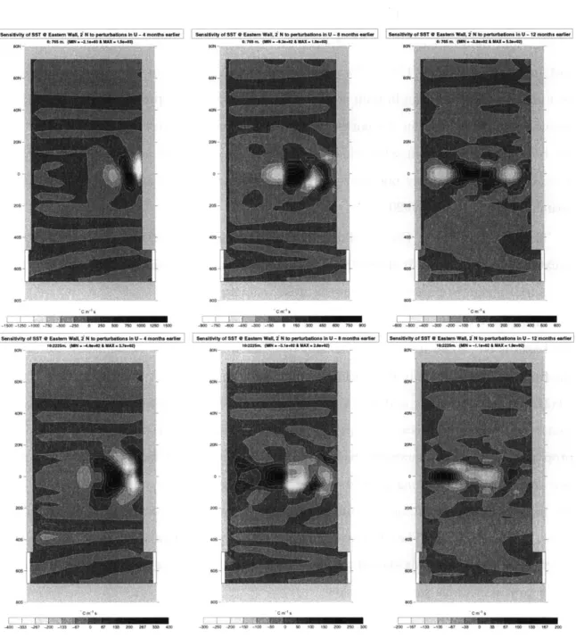
The adjoint model provides clear identification of the physical mechanisms which can influence the meridional overturning on times scales of years to decades. Boundary and equatorial Kelvin waves and equatorially trapped Rossby waves carry information around the boundaries of the basin and across the equator in less than a decade for a basin of the size of the Atlantic. Advection of buoyancy perturbations has an important influence on the meridional overturning on the decadal time scale. Diffusion is important in determining the final equilibrated state of the meridional overturning on the centennial scale.

The role of diapycnal mixing in determining the overturning's strength is confined to regions near the lateral boundaries in the Northern hemisphere and to the tropical region in both hemispheres. The important role played by the tropics in setting the overturning's strength seems to confirm the thermodynamic principles outlined by Sandstr6m (1908), Jeffreys (1925) and Munk and Wunsch (1998): upward advection of heat is balanced by downward diffusion. The strength of the meridional overturning is then determined by the power available to return the fluid to the surface across the ocean's stratification. Because the ocean is most strongly stratified in the tropics, the mixing process is most efficient in that region. Along the eastern boundary in the extratropics, the importance of diapycnal mixing is confined to a shallow layer at the base of the thermocline. The large vertical tem-perature contrast between the western and deep western boundary currents induces efficient mixing in that region. Surface wind stress has two effects on the ocean's stratification which concentrate the sensitivity in the eastern equatorial region. Ekman suction increases the stratification along the equator while Ekman pumping decreases it in the rest of the trop-ics. The equatorial easterlies lift the thermocline on the eastern side of the basin, further increasing the stratification and the efficiency of the vertical mixing process in that region. These processes are similar in the results from a coupled model. Atmospheric feedbacks do, however, allow vertical mixing in the Pacific to play a role as important as mixing in the Atlantic in determining the overturning's strength. The large uncertainties in the global value of the diapycnal mixing in the ocean, estimated here at , = 3. 10-5 ± 2 -10-5 m2s- 11

translate into an uncertainty of approximately 6 Sv in the maximum value of the meridional overturning streamfunction.

The role of surface buoyancy forcing on the overturning's strength depends on the for-mulation of the surface boundary conditions. The sensitivities are confined to high latitudes and the vicinity of convection sites when the surface forcing is prescribed as restoring the sea surface salinity or temperature towards observations. When the forcing is prescribed as a flux of heat or freshwater, advection allows buoyancy perturbations in the Atlantic basin to play an important role in determining the evolution of the meridional overturning. For annual and decadal time scales, heat flux perturbations in the North Atlantic are likely to

have the greatest impact on the meridional overturning. On climatological time scales, it is the uncertainty in the precipitation and evaporation fields in the tropics which have the greatest impact on the uncertainty in the streamfunction, the latter can be estimated at:

'MAX = 29 ± 4 Sv. Over the intermediate time scale of climate change, the overturning

is likely to weaken at first because of warming and freshening in high latitudes. It will, however, eventually recover as positive salinity anomalies are advected northwards from the tropics.

The sensitivity of the overturning to the wind stress forcing is also dependent on the surface boundary conditions. Under restoring boundary conditions, large positive sensitiv-ities are observed in the Antarctic Circumpolar Channel in a pattern reminiscent of the so-called Drake Passage effect. According to that hypothesis, upwelling of North Atlantic Deep Water takes place predominantly in a branch of the Deacon cell in the Drake Passage region. The importance of wind in the Drake Passage vanishes when the surface buoy-ancy fields are less tightly constrained, for example in the model forced by mixed boundary conditions or in the coupled model. The Agulhas Plateau, the Chilean coastline and the Indonesian throughflow play an important role in setting the overturning's strength in the ocean model forced by mixed boundary conditions. These "gateways" act as a regulator of the salinity of the Atlantic basin. The wind stress determines the balance between the inflow of relatively salty Indian Ocean water through the Agulhas current, the inflow of fresher Benguela current water southwest of Africa and the flow of very cold and fresh water through the Drake Passage. A wind stress perturbation of ±0.03 N m 2 over the Agulhas Plateau would have a significant impact on the meridional streamfunction's

maxi-mum, estimated at OpMAX = 29t+0.5 Sv. Both Drake Passage and gateway effects disappear

almost completely in the coupled version of the model, which shows the strongest positive sensitivities to wind stress in the region of equatorial Ekman upwelling.

Our study shows that, in a climatological ocean model, the choice of air-sea boundary conditions is crucial in determining the sensitivity of the meridional overturning circulation. The climatology of the forward ocean model is credible and quite similar in all scenarios. However, including interactive atmospheric transports of heat and moisture changes the manner in which the ocean model state adjusts to changes in wind stress, heat flux and diapycnal mixing. Considering the role of both the atmosphere and the ocean when studying the climatological behavior of the MOC is, therefore, clearly important. Models which keep one of the components fixed can lead to very different conclusions from models in which both components are represented.

Thesis Supervisor: Peter H. Stone Title: Professor

Acknowledgements

To my great-grandmother Florence for her sense of humor, To my grandmother Perle for her sense of dedication, To my mother Jacqueline for her love.

Without a solid sense of humor, dedication to the task at hand and the love of those around me, I don't know if I would have finished what I set out to do five years ago when I first came to MIT. This thesis is dedicated to three generations of exceptionally bright women who came before me and paved the way.

Like my great-grandmother, I like to smile at most things. Humor at MIT belongs to the students; it's how we manage to laugh at the hoops we are made to jump through. I have been very fortunate to meet some of the best, brightest and nicest people from the four corners of the world. Gerard Roe, who introduced me to MIT, then spent three years trying to convince me that warm beer was actually good; Kerim Nisancioglu and Sussie Dalvin, who every day reminded me that there is life beyond work and Jessica Neu, my favorite training partner, with whom I have shared the joy and tears of being a girl, albeit a tough one, lost in a man's world. Many thanks to my housemates Cindy Kiddoo and Jake Gebbie for allowing me to ramble on late at night on just about anything; I now know more about the brain and the art of skateboarding than I ever thought I would. Much gratitude goes to my officemates over the years, Amy Solomon, Tieh-Yong Koh, Peter Huybers and Baylor Fox-Kemper for having answers to just about anything. To my fellow "staff meteorologists" at the Tech, Greg Lawson, Rob Korty, Bill Ramstrom, it's the best title we will ever have. Thank you to Helen Johnson, Sarah Samuel and Karen Mair for reminding me of the old continent, or at least the island off the old continent, and for many great hiking, kayaking and climbing trips. Francesca Scirre-Scapuzzo and Joe Seidel, thank you for bringing a little bit of home over to Boston. To my classmates, Galen McKinley, Juan Botella, Pablo

Zurita, Yu-Han Chen, Jelena Popovic and Don Lucas for being such a fun and diverse group of people. Thank you Zan Stine and Nili Harnik for being who you are, please don't change. To my favorite skiing, sorry, telemark, buddies Peter Madden, Adam Lorenz and the rest of the 529 gang for teaching me that bruised knees really don't matter.

Without an inordinate amount of dedication, finishing a thesis would be a difficult task.

My grandmother taught me from an early age the meaning of that word. I have the greatest

respect for my thesis committee, Glenn Flierl, Carl Wunsch, Jochem Marotzke and John Marhsall, for their dedication to science. I am particularly indebted to John Marshall who volunteered to join my committee at the last minute and whose endless enthusiasm for science has made a lasting impression upon me. I would like to thank my advisor, Peter Stone, for his advice and generous support of my academic, and sometimes not-so-academic career; field work in the Canadian Arctic and a summer working on the world's first french windstorm bond were great breaths of fresh air. Without Jane McNabb, Mary Elliff, Maria Raposo and Gail Hickey's dedication to students, the sky would have often been less blue in the morning. I cannot thank enough Linda Meinke for her technical assistance, and for her ability to always recuperate files mistakenly sent to the wastebasket and Will Heres for many great lunchtime conversations and for always keeping the printer working. Thank you to all the people who have contributed to the ocean model and the black box called the adjoint compiler: Alistair Adcroft, Ralf Giering, Patrick Heimbach and the staff of the ECCO project at Scripps and JPL. I am indebted to Xiaoli Wang for laying the groundwork of this project and to Jeff Scott for his patience in teaching me the secrets of ocean mixing. I was very lucky to work with a very bright, but also very nice person, Chris Hill, who insisted on building the world's most complicated computer on the 1 7th floor of the Green building; he has taught me that research can be fun. I was honored to be involved with two very creative programs. The Technology and Policy Program showed me that the word interdisciplinarity really does exist. My thanks go to Jake Jacoby, the heart and soul of the Joint Program on the Science and Policy of Global Change, for his endless enthusiasm and for being a role model to so many of us. I am grateful to Mr. "Uncertainty in global warming" - Mort Webster - for all the free lunches, Chris Forest for many interesting discussions and Andrei Sokolov for the data. David Reiner, plasma physicist turned political scientist, thank you for being a great friend, for teaching me about all matters political, and for editing footnote

The love of your family is what remains in the moments when humor and dedication are not quite enough to finish the task at hand. To Andy for his near-infinite patience and wisdom, for being my favorite arctic sidekick and for not falling through the ice in Ross Bay. To my parents, Jacqueline and Jean-Robert, and my brother Edouard, for showing great interest in my work through endless newspaper articles on climate change and other energy problems, and for keeping track of all the funny symbols in my thesis. Without their encouragements, and their constant source of support, I would not be writing this today.

Contents

1 Introduction 25

1.1 Heat Transport in the Atmosphere and the Oceans . . . . 25

1.2 The Stability of the Meridional Overturning Circulation . . . . 26

1.3 Sensitivity Studies . . . . 28

1.4 Climate Predictability . . . . 30

1.5 Outline of the Thesis . . . . 31

2 Adjoint Dynamics 33 2.1 Introduction . . . . 33

2.2 Theoretical Background . . . . 34

2.3 Implementation . . . . 36

2.4 Description of the Forward Model . . . . 39

2.5 Equilibration Process . . . . 43

2.5.1 Time Scales of Equilibration . . . . 43

2.5.2 Adjoint Kelvin Waves . . . . 46

2.5.3 Adjoint Rossby Waves . . . . 53

2.5.4 Summary of the Role of Waves in the Equilibration Process . . . . . 56

2.5.5 Adjoint Advection . . . . 58

2.5.6 Adjoint Diffusion . . . . 62

2.6 Summary and Discussion . . . . 62

3 Adjoint Sensitivities and Surface Forcing 65 3.1 Introduction . . . . 65

3.2 Diagnostic Analysis using Green's Functions . . . . 66

3.3.1 Circulation . . . . 68

3.3.2 Cost Function . . . . 68

3.3.3 Diapycnal Mixing . . . . 69

3.3.4 Isopycnal Mixing and Thickness Diffusion . . . . 76

3.3.5 Relaxation Temperature and Salinity . . . . 79

3.3.6 Summary of Findings . . . . 81

3.4 The Role of Wind Forcing . . . . 81

3.4.1 Circulation . . . . 82

3.4.2 Diapycnal Mixing . . . . 82

3.4.3 Isopycnal Mixing and Thickness Diffusion . . . . 87

3.4.4 Wind Stress . . . . 89

3.4.5 Relaxation Temperature and Salinity . . . . 92

3.4.6 Summary of Findings . . . . . . . . 92

3.5 The Role of Heat and Freshwater Forcing . . . . 93

3.5.1 Circulation . . . . 94

3.5.2 Diapycnal Mixing . . . . 94

3.5.3 Wind Stress . . . . 100

3.5.4 Precipitation and Heat Flux . . . . 102

3.5.5 Isopycnal Mixing and Thickness Diffusion . . . . 108

3.6 Summary and Discussion . . . . 110

4 Model Description 113 4.1 Ocean Model . . . . 113

4.2 Energy and Moisture Balance Atmosphere . . . . 114

4.2.1 Heat Flux . . . . 114

4.2.2 Freshwater Flux . . . . 116

4.3 Model Spinup and Coupling . . . .. . . . . 117

4.4 Equilibrated State . . . . 119

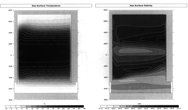
4.4.1 Temperature . . . . 119

4.4.2 Salinity . . . . 121

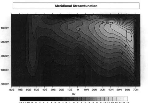
4.4.3 Meridional Overturning Circulation and Oceanic Heat Transport . . 122

5 What Drives the Overturning 5.1 Introduction . . . ..

5.1.1 Rate Limiting Mechanism

5.1.2 Application of the Adjoin

5.1.3 Cost Functions . . . . .. 5.1.4 Sensitivity to Time Deper

5.2 Buoyancy . . . .. 5.2.1 Model Results . . . . .. 5.2.2 Discussion. . . . .. 5.3 Mixing . . . .. 5.3.1 Model Results . . . . .. 5.3.2 Discussion . . . .. 5.4 Southern Oceans . . . .. 5.4.1 Model Results . . . . .. 5.4.2 Discussion . . . ..

5.5 Western Boundary Current . .

5.6 Quantitative Comparison . . . 5.6.1 Buoyancy . . . .. 5.6.2 Mixing. . . . .. 5.6.3 Wind Stress . . . .. 5.7 Discussion . . . .. 129 . . . . 129 as . . . . 129 it . . . . . . . . . . . . . . . . . . . . . . . . 130 . . . . 131 ndent Forcing . . . . 132 . . . . 133 . . . . 134 . . . . 141 . . . . 143 . . . . 143 . . . . 144 . . . . 148 . . . . 148 . . . . 160 . . . . 161 . . . . 161 . . . . 162 . . . . 164 . . . . 166 . . . . 167 6 Conclusion 171 181

List of Figures

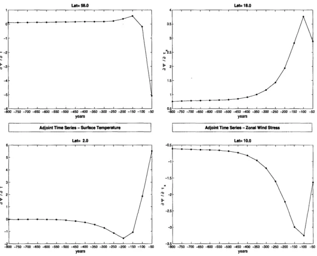
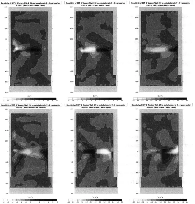
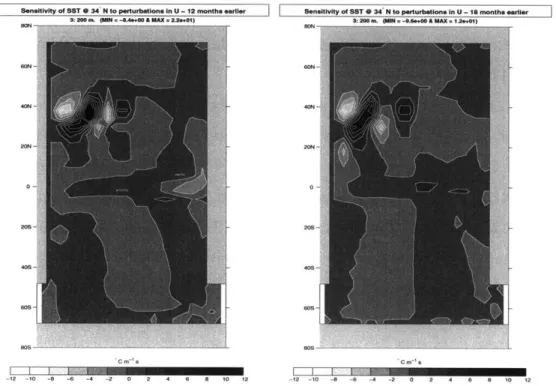
Two-level checkpointing . . . . Sea surface temperature and salinity in the single basin model . . . Circulation in the single basin model . . . . Meridional overturning streamfunction in the single basin model . Time series of the sensitivity of streamfunction maximum to the ir surface temperature and to wind stress . . . . Illustration of wave motion in an adjoint model . . . . Sensitivity of T(58' N, East) to u . . . . Sensitivity of T(2' N, East) to u . . . . Sensitivity of T(2' N, West) to u . . . . Sensitivity of T(34' N, 120 E) to u . . . . Time series of the sensitivity of the MOC to wind stress . . . . Time series of the sensitivity of the MOC to the surface heat flux .

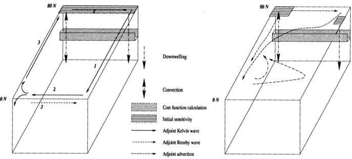
2-13 Summary of the pathways over which information is communicated

adjoint model . . . . nitial sea . . . . 45 . . . . 49 . . . . 50 . . . . 52 . . . . 54 . . . . 55 . . . . 57 in the

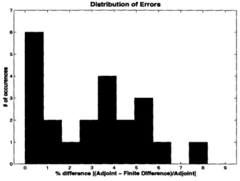
3-1 Distribution of the difference between the finite difference and the adjoint estimate of the sensitivity for 22 randomly sampled points and variables. . 3-2 Sensitivity of the maximum value of the streamfunction 1'MAX to the

diapy-cnal

This figure represents the response of a perturbation applied throughout each water colum n. . . . . 2-1 2-2 2-3 2-4 2-5 2-6 2-7 2-8 2-9 2-10 2-11 2-12 I. I

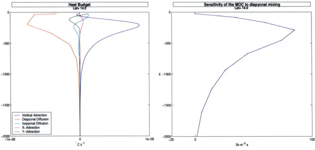
3-3 Left: Vertical profile of the heat budget at 140 N in the the middle of the

basin, all curves are in 'C m 1 s. The blue line represents vertical heat ad-vection: wTz; the red line represents diapycnal heat diffusion: ~ nTzz;the light blue line represents isopycnal heat diffusion: ~ ni(Tz + Tyy) the pink and green lines represents respectively heat advection in the x- and y- direc-tions: uT2, vTy; Right Vertical profile of the sensitivity to diapycnal mixing

a^MAX in Sv m-2 s at 140 _{N in the middle of the basin. Both plots represent}

d

the flow under relaxation boundary conditions with no wind forcing. . . . 72

3-4 Left: North-South cross-section along the eastern wall of the vertical velocity, in 10-6 m s1 Right: North-South cross-section along the eastern wall of the sensitivity to diapycnal mixing

(aMAX

3-5 Left: North-South cross-section along the eastern wall of the vertical gradient of the vertical temperature gradient (Tzz), in 'Cm 2_{. Right: North-South}

cross-section along the western wall of the sensitivity to diapycnal mixing

(-MAX)

s. Both plots were calculated under relaxation boundary conditions with no wind forcing . . . . 75

3-6 Sensitivity of the maximum value of the streamfunction IMAX to the isopyc-nal mixing and thickness diffusion: -a1 AX + a&MAX 8 inSm-2 s; Relaxation

Ktd in S

boundary conditions, no wind. This figure represents the response of a per-turbation applied throughout each water column. . . . . 77

3-7 Sensitivity of the maximum value of the streamfunction OA'AX to the relax-ation sea surface temperature: '9

?PMAX in SvC 1 (left) and to the relaxation

-9Tob.

sea surface salinity a x in Sv (right); Relaxation boundary conditions, no

wind... . . . . ... . . ... 79

3-8 Vertical section of the second derivative of the vertical temperature profile along the 20 N; Relaxation boundary conditions, wind and no wind . . . . . 83

3-9 Left: Vertical profile of the heat budget at 100 N in the the middle of the

basin, all curves are in 0Cm 1 s. The blue line represents vertical heat advection:wTz; the red line represents diapycnal heat diffusion: ~n dTzz;the light blue line represents isopycnal heat diffusion: ~ ni(Txx + Tyy) the pink and green lines represents respectively heat advection in the x- and y- direc-tions: uT, vTy. Right: Vertical profile at 2' N along the eastern boundary of the sensitivity to the diapycnal mixing (aOMAX ), in Sv m-2 s; Relaxation boundary conditions with wind forcing. . . . . 84

3-10 Sensitivity of the maximum value of the streamfunction "PMAX to the

di-apycnal mixing:

western boundary. Right: Sensitivity of the streamfunction maximum to diapycnal mixing op0 X in SV m-2 s along the western boundary.

. . . . .

isopyc-nal mixing: av'MAX in Sv m-2 s; Relaxation boundary conditions, wind. This figure represents the response of a perturbation applied throughout each

wa-ter colum n. . . . . 88 3-13 Left: Sensitivity of the streamfunction maximum to isopycnal mixing and

thickness diffusion avgMx in S M-2 s along the western boundary. Right: Meridional velocity along the western boundary in m s-I. . . . . 89

3-14 Sensitivity of the maximum value of the streamfunction IMAX to the zonal wind stress: '^MAX _Or, in Sv N-m 2; Relaxation boundary conditions, wind. 91

3-15 Sensitivity of the maximum value of the streamfunction OMAX to the relax-ation sea surface temperature and salinity: 090A .OSbX ; in SvoC1; Sv;

Relaxation boundary conditions, wind . . . . 92 3-16 Sensitivity of the streamfunction maximum to diapycnal mixing

(.PMAX

Sv m 2 s. Left: Restoring boundary conditions. Middle: Mixed boundary conditions. Right: Flux boundary conditions. The three plots are on the sam e scale. . . . . 95

3-17 Equilibrated response (AT in 'C) to a perturbation in diapycnal mixing

imposed at 380 N at the western boundary at a depth of 95 m: Arsd = 3 -10-6m2 -1 _{. Left: Mixed boundary conditions. Right: Flux boundary} conditions . . . . .. 3-18 Equilibrated response (AT in 'C) to a perturbation in diapycnal mixing

imposed at 38' N, 8' east of the western boundary at a depth of 500 m: And = 3- 10-6m2 ..- ...

3-19 Sensitivity of the streamfunction maximum to the zonal wind stress

(6VMAX

in Sv N- iM2. Left: Restoring boundary conditions. Middle: Mixed bound-ary conditions. Right: Flux boundbound-ary conditions. The three plots are on the same scale. . . . .. 3-20 Left: Observed zonal mean wind stress (-,), in N m-2. Right: Meridional

gradient of the zonal wind stress

(%),

(a9aMX

Sv W- 1M2 (top) and to the freshwater flux

(a_^X)

thick-ness diffusion

(&MAX

three plots are on the same scale. . . . . 108

4-1 Top: Ocean - atmosphere heat flux Qbs in W m-2. + Runoff - Evaporation in cm y-1 . . . . . 4-2 Sea surface temperature climatology . . . . 4-3 Sea surface temperature in the coupled model . . . . 4-4 Sea surface salinity climatology . . . . 4-5 Sea surface salinity in the ocean model . . . . 4-6 Sea surface salinity in the coupled model . . . . 4-7 Meridional streamfunction in the ocean model .. . . 4-8 Meridional streamfunction in the coupled model . . Bottom: Precipitation . . . . 118 . . . . 120 . . . . 120 . . . . 121 . . . . 123 . . . . 123 . . . . 124 . . . . 125 5-1 Illustration of three mechanisms thought to drive the meridional overturning

circulation. The thin lines represent the meridional streamfunction...

97 99 100 101 104 130

5-2 Sensitivity of the maximum value of the streamfunction IMAX to the heat

flux:a9'MX in SV W-1 m2 and to the freshwater flux: a9aMAX in Svm-- s in

the ocean model. The model's boundary conditions are F = (E - P - R)ob, and

Q

in the ocean model. The model's boundary conditions are F = (E-P-R)ob,

and

Q

5-4 Sensitivity of the maximum value of the streamfunction 1MAX to the heat

flux: aMAX in SvW-1 m2 in the coupled ocean, energy and moisture balance

model. The model's boundary conditions are F = (E - P)mod - Robs and

Q

fresh-water flux: aOMAX in Sv m--1 s in the coupled ocean, energy and moisture

balance model. The model's boundary conditions are Fw = (E -P)mod - Robs

and Q = Qmod + Am(T - Tzon). . . . . 139

5-6 Temperature at 1250 m in the coupled model . . . . 142

5-7 Sensitivity of the maximum value of the streamfunction ?PMAX to a column

by column perturbation in the diapycnal mixing in the ocean model. Top:

9

MAX in SV m- 2

s. Bottom: 9HT24,N in PW m-2 s. The model's boundary

49Kd a d

conditions are Fw = (E - P - R)ob, and

Q

by column perturbation in the diapycnal mixing: a90MAX in Sv m-2 sin the

coupled model. The model's boundary conditions are Fw = (E -P)mod -Robs

and

Q

=

Qmod + Am(T

-

Tzon).

..

-.

. . . 146

5-9 Sensitivity of the maximum value of the streamfunction PMAX to the wind stress, both zonal and meridional: av9PMAX in So N-1 m2 in the coupled ocean, energy balance model. The model's boundary conditions are Fw = (E

-P)mod - Robs and

Q

5-10 Sensitivity of the maximum value of the streamfunction PMAX to the wind

stress, both zonal and meridional: NIMAX in So N-1 m2 in the ocean model.

The model's boundary conditions are F = (E - P - R)obs and

Q

+

5-11 Sensitivity of the maximum value of the streamfunction I)MAX to the

isopy-cnal mixing and thickness diffusion: as)M^X in Sv m-2 s in the ocean model.

The model's boundary conditions are F, = (E - P - R)obs and

Q

As(T - Tbs)... ... ... 151

5-12 Sensitivity of the streamfunction maximum to the zonal wind stress

(aaX

in Sv N-1 M2. Left: Restoring boundary conditions. Middle: Mixed

bound-ary conditions. Right: Flux boundbound-ary conditions. The three plots are on the sam e scale. . . . . 152 5-13 Change in temperature, in 'C at 100m. for a perturbation in the surface

wind stress of Sensitivity of the streamfunction maximum to the zonal wind

stress A/r x = 0.001 Nm-2 imposed at 500 S above the sill. Left: Restoring

boundary conditions. Middle: Mixed boundary conditions. Right: Flux boundary conditions. . . . . 153

5-14 Surface currents around the African continent. Ocean model. . . . . 155 5-15 Top: Difference in salinity (in 10-3) between simulations with a wind stress

perturbation (Ar = 0.005 N m- 2

) imposed at 300 S (left) and 420 S (right),

both at 220 E, and an unperturbed simulation. Bottom: Difference in near surface currents (in m s1) between simulations with a wind stress perturba-tion (A-r. = 0.005 N m-2) imposed at 30' S (left) and 420 S (right), both at

220 E, and an unperturbed simulation. Ocean model. . . . . 156 5-16 Sensitivity to diapycnal mixing and flow velocities in the Agulhas Plateau

region. . . . . 158 5-17 Sensitivity of the maximum value of the heat transport at 24' N HTMAX

to the zonal wind stress: HT24o" in PW N- 1M2 _{in the ocean model. The}

model's boundary conditions are F = (E - P - R)obs and

Q

+

-Tos).. ... . ... . . . .. ... .. . . . .. . . ... 159

6-1 Estimates of the effect of uncertainty in the heat and freshwater fluxes, wind stress and diapycnal mixing on the meridional overturning's strength. The area of each circle is proportional to its contribution to the uncertainty in

6-2 Estimates of the effect of uncertainty in the heat, freshwater fluxes and

diapy-cnal mixing on the meridional overturning's strength for the ocean model. Solid green line: Effect of a 66% increase in diapycnal mixing, worldwide. Dash-dotted blue line: Effect of a 30% increase in freshwater flux (increased rainfall) between 540 N and 74' N in the Atlantic. Dashed blue line: Effect

of a 30% increase in freshwater flux (increased evaporation ) between 22' S and 220 N in the Atlantic. Dash-dotted red line: Effect of a 30% increase in heat flux (cooling of the ocean) between 540 N and 740 N in the Atlantic.

Dashed red line: Effect of a 30% increase in heat flux (warming of the ocean

) between 220 S and 220 N in the Atlantic. . . . . 175 6-3 Estimates of the effect of uncertainty in the heat and freshwater fluxes, wind

stress and diapycnal mixing on the meridional overturning's strength. The area of each circle is proportional to its contribution to the uncertainty in OMAX, in Sv. Top: The perturbations are maintained during ten years. Bottom: The perturbations are maintained during 25 years. . . . . 179

List of Tables

3.1 Formulation of the surface buoyancy forcing terms for mixed, restoring and flux boundary conditions. The bar refers to a zonal averaging over the Atlantic basin, obs, refers to a field derived from observations (Levitus and T.P.Boyer, 1994a,b; Jiang et al., 1999), ref refers to a reference salinity (35) and diag refers to a field, which has been diagnosed from the spinup under mixed boundary conditions. . . . . 93 3.2 Sea surface temperature, salinity and density perturbations induced by a

per-turbation in diapycnal mixing (Anaz = 3.10-6 m2 _s 1_{) applied one level below}

the surface at 2' N along the eastern boundary. The density perturbation was estimated by using the linearized equation of state. . . . . 96 3.3 Sea surface temperature, salinity and density perturbations induced by a

per-turbation in diapycnal mixing (And = 3-10-6 m2 _{s--1) applied one level below}

the surface at 380 N along the western boundary. The density perturbation was estimated by using the linearized equation of state. . . . . 98

3.4 Estimated effect (in Sv) on the maximum value of the meridional stream-function PMAX of a And = 3 -10-6 m2 s- perturbation in the diapycnal mixing applied throughout a specific region. . . . . 100 3.5 Estimated effect (in Sv) on the maximum value of the meridional

stream-function MAX of a ATr = 0.005 N m-2 perturbation in the zonal wind stress applied throughout a specific region. *: the perturbation was applied only over the eastern half of the basin. . . . . 102

3.6 Estimated effect (in Sv) on the maximum value of the meridional stream-function 'iMAX. Flux BC: AQ = 4 W m-2 perturbation in the net heat flux. Restoring BC: ASST = -0.1*C perturbation in the relaxation sea surface temperature. Mixed BC: combined effect of AQ = 2 W m-2 and

ASST = -0.05'C perturbations. . . . . 107

3.7 Estimated effect (in Sv) on the maximum value of the meridional

stream-function 'IMAX. Mixed and Flux BC: AP = 5.8mmyr-1 perturbation in the net precipitation field. Restoring BC: ASSS = 0.027 perturbation in the

sea surface salinity. . . . . 107 3.8 Estimated effect (in Sv) on the maximum value of the meridional

stream-function

OMAX

Ani

4.1 Heat transport by the ocean across key latitudes in Atlantic and Pacific basins, and globally . . . . 126

5.1 Uncertainty in the estimates of the overturning maximum OMAX estimated by applying perturbations in the heat and freshwater fluxes in various regions.

These perturbations are 30% of the value of the fields themselves. . . . . . 162 5.2 Uncertainty in the estimates of the overturning maximum @MAX estimated

by applying perturbations in the heat and freshwater fluxes in various regions.

These perturbations are AQ = ±30 Wm-2 and AF, = ±30 cmy-1 . . . . . 162 5.3 Impact of a 66% increase and decrease in the value of the diapycnal mixing

coefficient. . . . . 165

5.4 Boundary mixing hypothesis. An= 7 -10-5 m2S-1 along coastlines, And =

-3.

. . . .

5.5 Tropical mixing hypothesis. And = 7. 10--5 m2s1 _{between 22 - 6' S and}

6 - 220 N and above 1000m, And = -3 -10-5 m2 _-1 _{elsewhere. . . . . 166}

5.6 Uncertainty in the estimates of the overturning maximum PMAX estimated

by applying perturbations in the zonal wind stress. These perturbations are 30% of the value of the field. . . . . 167

5.7 Uncertainty in the estimates of the overturning maximum )MAX estimated

by applying perturbations in the zonal wind stress. These perturbations are ±0.03 Nm-2 of the value of the field. . . . . 167

Chapter 1

Introduction

1.1

Heat Transport in the Atmosphere and the Oceans

Without any transport of heat from the tropics to higher latitudes by the atmosphere and the oceans, the Earth would be approximately forty degrees colder at the poles and warmer

by the same amount at the Equator (North et al., 1981). The partitioning of this heat

transport between the atmosphere and the ocean changes from basin to basin, between hemispheres and with seasons (Peixoto and Oort, 1992). Only the total heat transport is known accurately, the ratio of oceanic to atmospheric heat transport is poorly known. Observations indicate that neither medium contributes more than two-thirds of the overall heat transport (Peixoto and Oort, 1992). It is also poorly known how efficiently the Earth can compensate an increase in heat transport in one medium by a decrease in the other. Large variations in historical temperature records suggest that this natural compensation mechanism is, at at best, imperfect.

The atmosphere transports heat northward in baroclinically unstable disturbances, pri-marily in mid-latitude storms, and in stationary waves. The ocean has essentially two methods for transporting heat northward. Considering first the deviations of the flow from its basin wide average, a warm northward anomaly or a cold southward anomaly both achieve a net transport of heat to the North. This is how the wind driven subtropical gyres contribute to the world's heat balance. The basin mean circulation will transport heat to-wards the pole if there is a poleto-wards warm flow near the surface and a colder equatorto-wards flow at greater depth. This circulation is referred to as meridional overturning circulation; it advects a large amount of heat from tropical latitudes towards the pole in the Atlantic

basin. The Atlantic ocean has the peculiar feature of transporting heat equatorwards in the Southern Hemisphere, primarily because of heat transport associated with the over-turning component. The polewards transport of heat by the gyres in the Pacific and Indian oceans is, however, polewards. Overall, observations indicate that the world's oceans trans-port heat polewards in both hemispheres (Trenberth and Solomon, 1994; Macdonald and Wunsch, 1996).

1.2

The Stability of the Meridional Overturning Circulation

The meridional overturning circulation, often referred to as thermohaline circulation or popularly as the ocean's conveyor belt, will be the focus of much of this thesis. The heat transported by this circulation is gradually released into the atmosphere, thereby giving Western Europe its comparatively mild climate. The intense cooling of the ocean surface in the Norwegian, Greenland and Labrador Seas leads to a localized convective overturning of the water column in those regions. The pressure gradients, which are thereby generated, drive the southward movement of the North Atlantic Deep Waters.

A seminal paper by Stommel (1961) pointed out that, in a simplified two-box illustration

of the meridional overturning circulation, two stable equilibria were possible. Sinking in the northern box corresponds to a thermally dominated circulation, the current situation in the Atlantic. The influence of salinity on the water's density dominates in the reverse circulation which sees sinking near the equator. Rooth (1982) revisited this issue and showed that the pole to pole density gradient can also have a significant influence on the direction and stability of the meridional overturning.

Since the work of Stommel, paleoclimate studies have pointed to disruptions of the thermohaline circulation as a possible explanation for the abrupt changes seen in the tem-perature records, which are reconstructed from ice and sediment cores (Broecker et al.,

1985). A popular theory explains the Younger Dryas cooling event, which took place

11,000-10,000BP, by a massive discharge of icebergs from the Laurentide ice sheet. The freshening of the surface waters in the Atlantic is thought to have led to a temporary shutdown, or at least a significant weakening, of one or several of the branches that form the North Atlantic Deep Water (Keigwin et al., 1992; Lehman and Keigwin, 1992).

sensitive to a large input of freshwater in the Northern North Atlantic (Bryan, 1986; Manabe and Stouffer, 1988; Marotzke and Willebrand, 1991; Rahmstorf, 1995). The simulation of climate change scenarios in coupled atmosphere-ocean general circulation models (GCMs) also show a gradually weakening circulation, attributed to enhanced northward atmospheric moisture transport in a warmer atmosphere and a subsequent freshening of the Atlantic (Manabe and Stouffer, 1994; Wood et al., 1999; Dixon et al., 1999). The dominance of changes in freshwater forcing over changes in the surface heat flux is, however, contested

by the results obtained with other models (Mikolajewics and Voss, 2000; Kamenkovich

et al., 2000b). Most studies have implicitly assumed that the meridional overturning's sensitivity to the surface fluxes of heat and water is geographically co-located with the sites of convection and downwelling, where the deep water is formed. The role played by the geographic distribution of the changes in forcing, the relative importance of changes in the tropics vs. high latitudes or of changes in the Atlantic vs. the Pacific are largely unknown. The role of pole to pole dynamics has received more attention. The work of Wang et al. (1999a,b), Scott et al. (1999) and Rahmstorf (1996) points to the freshwater flux in the South Atlantic as a possible regulator of the intensity of the meridional overturning circulation. The relative importance of oceanic and atmospheric transport mechanisms in determining the sensitivity of the meridional overturning circulation is also poorly known, although theoretical studies have shown that the atmosphere adds a number of positive feedback mechanisms, which tend to amplify disturbances in the overturning's strength (Nakamura et al., 1994; Marotzke, 1995). Other outstanding issues include the role played

by the rate of warming on the evolution of the overturning (Stocker and Schmittner, 1997;

Wood et al., 1999), and the presence of stability thresholds beyond which changes in the circulation become difficult to reverse (Rahmstorf, 1995; Zhang et al., 1999).

Past discussions have often implicitly or explicitly assumed that the mechanism respon-sible for controlling the intensity of the meridional overturning circulation was convective mixing and the downwelling branch of the circulation. While this may be true for short-term changes in the circulation, the energy required to return abyssal waters to the surface is thermodynamically the factor limiting the intensity of the steady-state meridional over-turning circulation (Sandstrdm, 1908; Jeffreys, 1925). A number of mechanisms have been suggested to provide this source of energy. The first focuses on vertical mixing of heat, particularly along coastal boundaries and mid-oceanic ridges, as the true driving force of

the circulation (Marotzke and Scott, 1999; Zhang et al., 1999; Huang, 1999). This mixing would realistically be the product of wind or tidally induced gravity wave breaking (Munk and Wunsch, 1998). Such small scale processes are not resolved by the coarse resolution ocean general circulation models of the type used in this thesis, which therefore parameter-ize mixing as a diffusive process. The second hypothesis has the Southern Oceans playing a crucial role in determining the intensity of the overturning. Because of the absence of continental barriers, there can be no net East-West pressure gradient and, therefore, no net geostrophically balanced North-South flow in the Antarctic circumpolar channel. The westerlies drive a northward Ekman drift in the near surface layers that does not need to be in geostrophic balance. To satisfy geostrophy, the return flow must take place below the depth of the topographic ridges, notably below the sill located between the southern tip of South America and Antarctica. The divergence of the Ekman transport south of the Drake Passage can thereby draw up an estimated 15 Sv of deep water from below the level of the topographic ridges. This, theoretically, provides the source of energy required to convert the cold and salty North Atlantic Deep Water, which is observed below the top of topographic ridges, into fresher surface water (Toggweiler and Samuels, 1995, 1998). This Deacon cell, and its associated upwelling, is largely eliminated from the meridional overturning circulation, when the eddy induced transport velocity is added to the Eulerian mean velocity (Danabasoglu and McWilliams, 1995). This additional "bolus" velocity is linked to the Gent-McWilliams parameterization. By adding a down-gradient diffusion of the thickness between isopycnal surfaces, this parameterization produces an effect that can be expressed as an additional tracer advection.

Only a sensitivity study, which includes all the elements forcing and constraining the ocean's circulation, has the potential to determine the relative influence of freshwater, heat fluxes, dia- and isopycnal mixing, thickness diffusion and wind stress on the intensity and stability properties of the meridional overturning circulation.

1.3

Sensitivity Studies

Traditional sensitivity studies are performed by adding small perturbations to the variables or parameters presumed to be important, and comparing the perturbed integrations to the control run. This method has the advantage of giving information about the impact of

the perturbation on all model variables during the integration period, its drawback is the limit to the number of parameters or input variables that can be examined. This constraint is imposed by the necessity to run one simulation for each perturbed parameter or initial condition, and the associated large computational requirement of the method.

Adjoint methods have the advantage of providing the sensitivity of a scalar function of the model state at a given time, often called cost function in optimization problems, to all model parameters and initial conditions in a single integration of the adjoint model. The use of adjoint methods to perform sensitivity studies in climate models was pioneered

by Hall & Cacuci in a sequence of papers in the early 80s (Hall et al., 1982; Hall and

Cacuci, 1983; Hall, 1986). They first applied it to a radiative-convective model of the atmosphere, demonstrating that the method was successful in deriving useful sensitivities, even though that model contained complex non-linear processes of the general type found in atmospheric and oceanic GCM's, notably episodic convective adjustment. The method was then tested on a greatly simplified atmospheric GCM showing that, within the limitations imposed by computational costs, deriving sensitivities useful to the interpretation of the results of climate models was a feasible task. In spite of their computational advantage over traditional perturbation methods, sensitivity studies using adjoint methods have largely been abandoned since Hall & Cacuci's efforts, primarily because of the necessity to write manually the code of the adjoint model. This daunting task has recently been greatly simplified by the advent of adjoint compilers which use automatic differentiation methods to generate the adjoint code (Giering, 1997). More recently, Marotzke et al. (1999) used automatic differentiation to derive the adjoint model of an ocean GCM, these authors examined the sensitivity of the heat transport in the Atlantic to the temperature and salinity distribution throughout the basin one year earlier.

Because they provide information about the gradient of a diagnostic with respect to the model state, adjoint methods have been used in data assimilation problems in atmosphere and ocean GCMs (Wunsch, 1996; Talagrand, 1997). The matrix composed of these gradients allows for the solution of the minimization problem that is required to constrain the flow to best correspond to observations.

Within the uncertainty in the model parameters, adjoint methods allow a ranking of the impact of changes in various model inputs on a given cost function. The adjoint method therefore provides the tool that allows to determine which of the competing influences on the

stability and intensity of the meridional overturning circulation plays the greatest role. A quantitative comparison of the effect of perturbations in the parameters on the overturning's intensity requires the multiplication of the sensitivities obtained with the adjoint model with a perturbation in the field or parameter. While the uncertainty in fields such as wind stress is quantifiable, other fields are much less precisely known. The globally averaged value of the diapycnal mixing is, for example, unknown to a factor of three or more (Gregg,

1987). Because of the linearization, which underlies the adjoint model, the validity of the

comparative analysis if furthermore limited to small perturbations in the underlying fields. Adjoint methods are, however, no substitute for traditional perturbation methods when the objective is to determine how these parameters affect the physical characteristics of the general circulation within the ocean model.

1.4

Climate Predictability

Adjoints have also been used in ensemble forecasting by the European Center for Medium Range Weather Forecasting (ECMWF) (Mureau et al., 1993; Palmer et al., 1994; Buizza et al., 1993; Buizza and Palmer, 1995; Molteni et al., 1996). In that scheme, the "singular vectors", provide the geographic locations where disturbances are most likely to grow over the time span of the weather forecast. The operator, which maps small perturbations in the atmosphere along the weather forecast's trajectory from the initial state to a future time is known as the forward tangent propagator. Singular vectors are the product of the forward tangent propagator with its adjoint with respect to an energy norm.

The suitability of this method is, however, limited to the time scale over which the perturbation growth remains linear, approximately three to four days in the atmosphere (Molteni and Palmer, 1993; Palmer, 1993a). It is unclear whether an equivalent time scale exists for slower ocean processes. The results of Wang et al. (1999b) suggest that the evolution of the thermohaline circulation, when forced by increasing fluxes of freshwater in high latitudes, is dependent on the sequence of random wind stress fluctuations. This result would imply that there exists a limit to the predictability of the evolution of the climate system. These results have, however, not been reproduced by other coupled climate models. Reconstructions of historical temperatures from ice cores or other paleoclimate data sources do, however, show important fluctuations on a number of time scales. It is unknown which

of these variations are predictable and which are not (Palmer, 1996). Addressing these questions requires climate models, which are sufficiently simple to be integrated over long time scales. It is also important that these models parameterize the transport of tracers such as heat, moisture or salinity by turbulent eddies. This requirement is due to the difficulty in obtaining useful adjoint sensitivities beyond the limit of predictability of the behavior of the individual eddy (Lea et al., 2000; K6hl and Willebrand, 2001). The use of non eddy resolving ocean models, such as the one used in the present analysis, may, however, limit the generalization of the results to more complicated eddy resolving systems. Provided that climate models show adequate intrinsic climate variability when forced by changes in orbital parameters, solar cycles, aerosol or greenhouse forcing, the singular vector method used for ensemble forecasting by the ECMWF could be used to gauge the predictability of the response of the climate system to these various types of forcing (Palmer, 1993b, 1999).

1.5

Outline of the Thesis

Chapter 2 gives a brief overview of the dynamics of the adjoint model. This chapter is provided to familiarize the reader with the mechanisms and time scales over which infor-mation is communicated around the basin in the adjoint model. This overview will include the dynamics of adjoint Kelvin and Rossby waves, as well as advection in the adjoint space. The focus of this chapter is entirely on time dependent processes.

Chapter 3 will provide a suite of experiments in an idealized single basin setting to develop an understanding of the steady-state sensitivity patterns provided by the adjoint model. Complexity is gradually built up by focusing first on the forcing by temperature and precipitation alone, while omitting the forcing of the momentum terms by the wind stress. The effect of wind is analyzed in a second series of experiments. The role played by the formulation of the surface buoyancy forcing terms is examined in a third set of calculations, highlighting the dependency of the model's response on how the surface forcing terms are calculated. The analysis will focus on the role of mixing, surface buoyancy forcing and when appropriate, wind stress forcing on the meridional overturning circulation.

Chapter 4 briefly presents the structure and flow characteristics of the simplified coupled ocean, energy and moisture balance atmosphere model. This model will be used to analyze, in chapter 5, the sensitivity of the meridional overturning circulation to surface forcing and

mixing in a realistic geography configuration. This chapter is structured by theme, and focuses on using the adjoint model to gain insight and provide support for the theories, which seek to explain the intensity of the overturning in terms of mixing, wind stress and buoyancy forcing. This chapter also outlines how uncertainty in the heat, freshwater and momentum fluxes can be used to provide a range of uncertainty in the model's estimates of the overturning's intensity and polewards heat transport in the Atlantic basin.

Chapter 6 reviews the major results of this thesis, but also emphasizes the limitations of the adjoint method. This chapter also outlines the direction of future research.

Chapter 2

Adjoint Dynamics

2.1

Introduction

The analysis of the sensitivity of the output of a climate model integration to the model's parameters can provide valuable help in interpreting the model results. It can, for example, allow a quantitative estimate of the impact of uncertainties in these parameters on the state of the model at the end of the integration. By 'parameter' is meant here the combination of the model's initial conditions as well as the constant physical parameters, which determine the model's evolution. The sea surface temperature at the time when the integration starts is an example of an initial condition, the model's viscosity or gravity are physical parame-ters. Sensitivities to initial conditions will be referred to as "initial value" sensitivities, the terminology will be "parametric" sensitivity in the case of constant parameters.

Traditional sensitivity analysis is performed by repeated integrations of the ocean or coupled general circulation model model, perturbing slightly the value of a single param-eter at each integration. Sensitivities are obtained by dividing the difference between the perturbed integration and the reference, unperturbed, run with the magnitude of the per-turbation itself. For complex models such as the one presented in this chapter, any extensive analysis using such a procedure is computationally unfeasible because of the number of pa-rameters involved. In practice, this means that only the few papa-rameters judged a priori as being the most important can be investigated.

Adjoint methods express the response of the model as a diagnostic or cost function of the model variables. The system of adjoint equations, developed from a differentiated form of the original model equations, allows the computation of the sensitivity of the diagnostic

to all model parameters in a single calculation. In contrast, the traditional approach gives the sensitivity of all the model variables to a single parameter.

The terminology "forward" model will be used when referring to the numerical ocean or coupled general circulation model. The numerical code derived from the forward model, which calculates the sensitivity of the cost function to the model parameters will be referred to as "adjoint" model.

2.2

Theoretical Background

The output of an adjoint model calculation gives the sensitivity of the cost function to the initial conditions as well as to the model's physical parameters. The cost function can be any scalar function of the model output, as long as it remains differentiable. This can, for example, be the sea surface temperature at one geographic location, the intensity of the meridional overturning circulation at a given time or the change in the amount of heat transported by the ocean over time.

The adjoint problem is easiest to pose for discrete time intervals, n = 0...N, which

conveniently represents time stepping in numerical oceanic and atmospheric models (see for example Talagrand (1997)). The evolution of the state vector yn between time steps 0 and n +1 can be represented from the composition of the mapping of the state at one time step onto the next:

Yn+1 = Cn(yn) = Co Cno --- Ci(yo) (2.1)

where

Yo = (To, So, o,po, po, a)

In the ocean model described later in this chapter, yn is comprised of the prognostic variables: temperature (T), salinity (S) and the three-dimensional velocity vector (a), the diagnostic variables pressure (p) and density (p) as well as the model's physical parameters (a). The variables are represented by three-dimensional arrays of the dimensions of the model grid, a is a vector of the same dimension as the number of independent parameters in the model.

6_{Yn+1 = C'n}6_{yn (2.2)}

C1nj= 0bY(i;n)

" a

Oy(J-n-1)

C' is often called the linear propagator, the index n represents time, ij are spatial

indices. C' exists only if the mapping is differentiable. Jyn is in turn related to the initial perturbation 6yo at time t = 0 through the repeated application of the rules of derivation

for the composition of functions:

gyn+1 = C'noyn = C'nC'n_1...C'16yo = C'6yo (2.3)

Cf 16Y(i;n)

0 6

y(j;o)

Equations 2.2 and 2.3 are a compact representation of the so-called tangent linear system of equations.

The gradient of the cost function, a response functional of the output state vector J(yN) at final time t = N, with respect to the model input obeys the following equation:

a

W

(2.4)

U(i'

0)

aY

O(i;0)

aY(j;N)

or in more compact notation:

Vy

J

where the superscript * indicates the use of the adjoint matrix. This follows from the properties of the inner product ( , ):

bJ

J

KcI*VYN,

J"6yo)

(2.6)

Equation 2.5 illustrates the fact that the adjoint model is integrated backwards in time: