n5'~
ugW
XNNW
t~j2t00tin004:D
ff.E-l'VD..
t~
w or-t
.f0
-g
pu,0;0Dz;0;d X t- .
ff;
MASSACHUSETTS
I~
~
NSTI!TUE
TECH
O
GY
A Dual-Ascent Procedure for
Large-Scale Uncapacitated Network Design by
A. Balakrishnan, T.L. Magnanti, and R.T. Wong
A DUAL-ASCENT PROCEDURE FOR
LARGE-SCALE UNCAPACITATED NETWORK DESIGN
A. Balakrishnan
Krannert Graduate School of Management Purdue University
T. L. Magnanti
Sloan School of Management Massachusetts Institute of Technology
R. T. Wong
Krannert Graduate School of Management Purdue University
May 1987
Supported by Grant #ECS-8316224 from the Systems Theory and Operations Research program of the National Science Foundation.
t
Supported in part by ONR contract #NOOO 14-86-0689 from the Office of Naval Research.
C
Abstract
The fixed-charge network design problem arises in a variety of problem contexts including transportation, communication, and production scheduling. We develop a family of dual ascent algorithms for this problem. This approach generalizes known ascent procedures for solving shortest path, plant location,
Steiner network and directed spanning tree problems. Our computational
results for several classes of test problems with up to 500 integer and 1.98 million continuous variables and constraints shows that the dual ascent
procedure and an associated drop-add heuristic generates solutions that, in almost all cases, are guaranteed to be within 1 to 3 percent of optimality. Moreover, the procedure requires no more than 150 seconds on an IBM 3083
computer. The test problems correspond to dense and sparse networks,
Introduction
The fixed charge network design model, which is a fundamental discrete choice design model, is useful for a variety of applications in
transportation, distribution, communication, and several other problem settings that make basic cost tradeoffs between operating costs and fixed
costs for providing network facilities (see Magnanti and Wong (1984)). The
fixed charge design model is deceptively simple. The basic ingredients are a
set of nodes and a set of uncapacitated arcs, and, between selected pairs of nodes, a required flow that must be routed over the network. Each arc has two types of cost: a per unit flow cost and a fixed charge for using the arc. The problem is to select a subset of arcs that minimizes the sum of the flow (or routing) costs and fixed charge costs.
Magnanti and Wong (1984) have shown that the basic fixed charge design model is quite flexible and contains a number of well-known network
optimization problems as special cases including the shortest path, minimum spanning tree, uncapacitated plant location, Steiner network, and traveling salesman problems.
Since many of these special cases, e.g., the uncapacitated plant location problem, are known to be difficult to solve (in the parlance of computational complexity theory, they are NP-hard), so is the general fixed charge design
model. The closely related budget network design problem, that removes the
fixed charge terms from the objective function, but instead limits the sum of fixed charges incurred through a budget constraint, is also NP-hard (Johnson,
Lenstra, and Rinnooy Kan (1978)). In fact, Wong (1980) has shown that even
finding an approximate budget design solution is an NP-hard problem.
In addition to these theoretical arguments, substantial empirical
evidence also confirms the difficulty of solving network design problems. A
number of researchers including Hoang (1973), Boyce, Farhi and Weischedel (1973), Dionne and Florian (1979), Boffey and Hinxman (1979), Gallo (1981) and Los and Lardinois (1980) have studied branch and boiind algorithms for either
the fixed charge or budget design problems. Although these branch and bound
algorithms can successfully solve problems with a small number of arcs (up to 40-50), their computation time grows very quickly in the problem size.
For larger scale problems, several approximate solution procedures are
available. Billheimer and Gray (1973) and Los and Lardinois utilize add-drop
type heuristics for the fixed charge design problem; Dionne and Florian, and Boffey and Hinxman use similar techniques for the budget design problem. Wong (1985) describes a special add heuristic for budget design problems on the Euclidean plane. He shows that asymptotically it is very likely that the cost of the solution generated by this heuristic will, under certain conditions, be very close to the cost of the optimal solution.
Some recent research has extended the range of applicability of
optimization-based approaches. Magnanti, Mireault and Wong (1986) have solved
network design problems with an accelerated version of Benders' decomposition combined with a preprocessing routine that eliminates unnecessary variables. The preprocessing routine utilizes a dual ascent procedure to be described in
this paper. This implementation of Benders' method has been able to solve to
optimality undirected network problems with up to 30 nodes and 90 candidate
arcs. Lamar, Sheffi and Powell (1984) have proposed an iterative
linearization scheme embedded in a branch and bound routine. The algorithm has been successfully applied to a special type of fixed charge directed network design problem that arises in freight routing operations. The test problems include networks with up to 46 nodes and 510 fixed-charge arcs.
In this paper we present a new dual-based approach for solving large-scale fixed charge network design problems. We begin in Section 1 by modeling the fixed charge design problem as an integer program and discussing various
formulations, including a new one for the undirected network case. Section 2 describes dual ascent procedures for computing approximate solutions to the dual of the linear programming relaxation of the design problem formulation. The dual solution provides a lower bound for the optimal solution value and this solution, together with the complementary slackness conditions, permits us to generate a feasible network design solution. By using a drop-add
heuristic, we further improve the upper bound generated by the feasible design solution. The dual lower bound, when used in conjunction with the upper bound from the heuristic solution, enables problem reduction by eliminating some arcs from the network. Section 3 presents these and other enhancements.
As part of our discussion in Section 2, we also comment on some general principles for designing dual ascent algorithms. We show how our ascent
-procedure can be viewed as a generalization of Dijkstra's (1959) shortest path algorithm and of Wong's (1984) dual ascent procedure for the Steiner network problem, which itself generalizes Bilde and Krarup's (1977) and Erlenkotter's (1978) ascent algorithm for uncapacitated plant location, as well as the Chu-Liu (1965) and Edmonds (1967) directed spanning tree algorithm. Thus, just as the network design model formulation generalizes the shortest path, facility
location, spanning tree and Steiner network problems, our algorithm generalizes the dual ascent methods proposed for these special cases.
Finally, in Section 4, we present extensive computational results for our dual-based procedure on a wide variety of randomly generated test problems,
including sparse and dense networks containing up to 45 nodes and up to 595 candidate arcs. We also describe our experience in applying the method to solve some special design problems studied by Lamar, Sheffi and Powell (1984) in the setting of freight routing systems.
The dual based approach, with but a few exceptions, has been able to generate upper and lower bounds that differ by at most only 1 to 3 percent. The maximum CPU time required for the entire dual-based procedure was 150 seconds on an IBM 3083 -(model BX) computer. The dual ascent component of this procedure is quite efficient; for larger problems, the add-drop heuristic
consumes a major portion of the required CPU time.
In the past, dual ascent procedures have been successfully used to solve several special cases of the network design problem including the
uncapacitated plant location and Steiner tree problems. Our results, which show that the dual ascent approach can be successfully applied to a variety of large-scale network design models, confirm the power of the dual ascent
solution strategy and demonstrate the effectiveness of the approach for a broader range of network optimization problems.
1. Network Design Problem Formulations
This section introduces and discusses formulations for the general fixed charge network design problem. We focus on the undirected network case and give some alternative formulations including a new formulation when the flow
costs are the same for all commodities. Sect-ions 2 and 3 introduce algorithms
that utilize these network design formulations. All our subsequent
discussions apply with minor modifications to the directed network design problem as well.
1.1 General Network Design Model
The basic ingredients of the model are a set N of nodes and a set A of uncapacitated and undirected arcs that are available for designing a network. The selection of those arcs to be included in the network depends upon
tradeoffs between fixed design costs and variable operating costs. Selecting
more arcs offers the potential for reducing the operating (or routing) costs
at the expense of higher fixed costs. On the other hand, with fewer arcs in
the design, the fixed costs are lower but the routing costs increase.
The model permits multiple commodities which might represent distinct physical goods, or the same physical good but with different points of origin
and destination. (Some authors, e.g., Rardin and Choe (1979), Rardin (1982),
and Lamar, Sheffi and Powell (1986), permit commodities to have multiple
origins and destinations. Our model assumes, however, that each commodity has a single origin or single destination, which we model as a set of commodities, each with a single source and single destination.) We let K denote the set of
commodities and for each k K, assume (by scaling, if necessary) that one
unit of flow of commodity k must be shipped from its point of origin, denoted O(k), to its point of destination, denoted D(k).
The model contains two types of variables, one modeling discrete design choices and the other modeling continuous flow decisions. Let yij be a binary
variable that indicates whether (yij = 1) or not (ij = 0) arc i,j} is chosen
k
as part of the network's design. Let xk. denote the flow of commodity k on
the directed ar (ij). Note that (ij) and (ji) denote directed arcs with
the directed arc (i,j). Note that (i,j) and (j,i) denote directed arcs with
-opposite orientations corresponding to the undirected arc i,j). Even though arcs in the model are undirected, we refer to the directed arcs (i,j) and
k
(j,i) because the flows are directed. Then, if y = (Yij) and x = (x j) are vectors of design and flow variables, the model becomes
[P1]
minimize (ckijxij + cixji) + F iyij (l.1)
LJ I ljJ ji ji jij ksK ei,jc}A [i,j}EA subject to x i - Xil = jeN IN '-1 if i = O(k) all i N, and 1 if i = D(k) (1.2) all k K, 0 otherwise
L-xi - ij all i,jj e A, and (1.3a)
k all k K,
Xji < Yij (1.3b)
k k
xk., x.. > 0 all {i,j} e A, and
y. = °or 1 all k £ K. (1.4)
ij
In this formulation each arc i,j} has a nonnegative fixed design cost k
F.. and c.. is the nonnegative per unit cost for routing commodity k on the
k k
directed arc (i,j). In general, c.. need not equal c..i Constraints (1.2)
imposed upon each commodity k are the usual network flow conservation
equations. The "forcing" constraints (1.3a) and (1.3b) state that ifij = 0, i.e., if arc {i,j) is not included in the design, then the flow of every
commodity k on this arc must be zero in both directions, and if arc i,j is included in the design, i.e., if yij = 1, the arc flow is unlimited (since the flow of any commodity k on arc (i,j) or (j,i) is at most 1 anyway).
For directed network design problems, A is the set of available directed
arcs and Fij represents the fixed charge of the directed arc (i,j). The
k
formulation uses design variables yij for all (i,j) A and flow variables xi..
for all (i,j) A and k K. Inequalities (1.3a) defined for all (i,j) A
and k K constitute the forcing constraints for this case. The flow
conservation equations (1.2) remain unchanged, and the summations in the objective function are now taken over (i,j) rather than i,jj (and the terms
kk
c..kx are removed).
jixji
The network design problem can also be formulated in a number of
different ways. For example, aggregating the forcing constraints (1.3) yields the equivalent set of constraints
Z
xi; + xji < 2 K yij for all {i,j] A. (1.5)k
k k
Both versions of these constraints force each x.. and x.. for k 1 K to be zero
J J1
if yi] = 0, and become redundant if yi = 1. This alternate formulation is
much more compact, however. For one of the problems considered in our computational tests, with 1980 commodities and 500 arcs, the disaggregate formulation contains nearly 2 million forcing constraints (1.3), while the aggregate version contains only 500 of these constraints (1.5).
In addition, it is possible to aggregate commodities by origin (or k
destination). In this aggregate formulation, x, which now denotes the total
flow on arc (i,j) that originates at node k, corresponds to the aggregation (sum) over all destination nodes of the commodities with origin k. The forcing constraint becomes
k < and kNy
xij INli and xji <NlYij,
and the flow balance constraints (1.2) are altered accordingly (that is, the flow balance constraints for aggregate commodity k impose a requirement of 1 unit for each demand node D(1) in the original formulation whose origin 0(1)
is node k). For the problem mentioned in the last paragraph, this aggregate
formulation contains 45 rather than 1980 commodities and 45,000 rather than
nearly 2 million forcing constraints. (Note that it is also possible, as we
-do in our modeling approach, to reverse this procedure and disaggregate any commodity naturally formulated with a single origin and multiple destinations as a set of commodities, one for each destination.)
Although the disaggregate formulation contains a considerably larger number of constraints than either of these two aggregate formulations, it is
preferred computationally (if it can be solved efficiently). The linear
programming relaxation of the disaggregate model is much more tightly constrained than the linear programming version of the aggregate models. Therefore, the disaggregate formulation more closely approximates the integer program and provides a sharper lower bound on the value of the integer
programming formulation. Various authors have noted the important algorithmic
advantages of using tight linear programming relaxations. For example, see
Cornuejols, Fisher and Nemhauser (1977), Davis and Ray (1969), Beale and Tomlin (1972), Geoffrion and Graves (1974), Mairs et al. (1978), Magnanti and Wong (1981), Rardin and Choe, and Williams (1974).
As a final observation concerning the problem formulation (1.1) - (1.4), note that (since the problem is uncapacitated) for a given choice of binary design variables ij., the problem decomposes into a shortest path problem
(defined on the network specified by arcs with yij = 1) for each commodity. Therefore, the problem always has an optimal solution in which all the x
variables are integer. Our subsequent analysis and algorithmic development
makes heavy use of this problem feature.
1.2 An Improved Formulation for Fixed Charge Network Design
Under certain conditions, the linear programming relaxation of the disaggregate formulation (1.1) - (1.4) can be further tightened with another
version of the forcing constraints (1.3). We focus upon undirected network
k
design problems whose flow cost does not vary by commodity, i.e., c.. = c..
1J 1J
for all k K, and c.. + c.. > 0 for all 1 i,j} A. Many network design
J Ji
models satisfy this rather mild assumption.
Consider an arc [i,j] e A and two commodities k and h with origins O(k)
and O(h) and a common destination D(k) = D(h), which, for convenience, we assume is node 1. Suppose we have an optimal solution (x,y) to the integer
program P1 that routes each commodity k on a shortest path (see our final
k h
comment in Section 1.1), and x23 = 1. Then it is always possible to set x3 2 =
O and maintain optimality. To see this result, let d.. denote the minimum
1J
routing cost from node i to node j as defined on the network specified by the k
optimal choice of the Yij variables. Since x23 = 1 in the optimal solution
and the flow between every origin-destination pair is carried on shortest
paths d21 = 23 + d31. If x3 2 = 1, then the total routing cost for commodity
h will be
dO(h),3 c32 21 d(h),3 + c32 c23 d31
dO(h),3 + d3 1 (since c32 + c23 > 0),
h
Therefore, we can set x3 2 = 0 without loss of optimality. Similarly, we can
reverse the roles of x 3 and xh2 and, therefore, the constraint
23 32
xk+ h < 1
x23 x32
-will not affect the value of the optimal solution of the design model. In
general, this inequality becomes
xk + xh < y for all {i,j]eA if D(k)=D(h). (1.6)
xi]
i - ijThe same type of argument applies when commodities have a common origin O(k) = O(h); so we also have
k h
xkj + Xji < Yij for all {i,j}cA if O(k)=O(h). (1.7)
Notice that when h = k, (1.6) and (1.7) reduce to
Xkl + Xkj < Yij for all i,j}eA, kK.
ii i - ij
Since the flow variables are nonnegative, these inequalities are at least as
tight as (1.3). So if we substitute (1.6) and (1.7) for (1.3),the linear
programming relaxation of the resulting formulation P2 will be at least as
tight as LP1, the linear programming relaxation of P1.
LP2, the linear programming relaxation of P2, can be strictly tighter
than LP1. Consider, for example, the 3-node network shown in Figure 1.1, with
8
Figure 1.1
Example for Comparing LP1 and LP2
F
12=1
C12 =0 F13 = 1 C13 =0F
23= 1
C2 3 = 0Commodity
k
h
Origin
Destination
2
1
3
1
F12 = F13 = F23 = 1 and c..ij = 0 for all i,j). Suppose that the problem contains two commodities k and h with origins O(k) = 2, O(h) = 3 and
destinations D(k) = D(h) = 1. For this problem, the optimal solution to LP1
is
k k k h h h
12 Y13 23 = x2 1 = x23 = x3 1 = X21 = X3 1 = X3 2 = 1/2.
The total solution cost is 3/2. Notice that this solution violates the
constraint k constraint x + + h 3k 2 < Y23 from (1.6). An optimal solution to LP22 is
k h
Y12 = Y13 = x2 1 = 3 1 = 1
which has a total solution cost of 2. Hence, LP2 is strictly tighter than LP1
for this example.
For clarity, we first discuss solution methods for the original
formulation P. Section 2 introduces a general dual ascent framework for
approximately solving the dual of LP1, the linear programming relaxation of
problem P. We present two alternative implementations of the general dual
ascent strategy, and demonstrate how these algorithms generalize the ascent methods proposed earlier for some special cases of the network design problem. Section 3 deals with algorithmic modifications to handle the tighter
constraints (1.6) and (1.7), and other enhancements.
-2. Dual Ascent Algorithms for the NDP
Since the network design problem is NP-hard, we focus on methods for generating good lower bounds and heuristic solutions, rather than solving the problem optimally. The network design problem's special structure makes it a particularly attractive candidate for applying dual ascent, a technique that attempts to generate good lower bounds relatively fast by solving the linear
programming dual problem approximately. Besides generating lower bounds, dual
ascent solutions can also be used to identify feasible network designs that serve as starting solutions for local improvement heuristics. Further, they can aid in reducing the problem by eliminating some design variables.
Dual ascent has been applied successfully to several network design related models including the uncapacitated facility location problem (Bilde and Krarup, Erlenkotter, Van Roy and Erlenkotter (1982)), the generalized assignment problem (Fisher, Jaikumar and Van Wassenhove (1986)), the Steiner tree problem (Wong (1984)), the set covering problem (Kedia and Fisher
(1986)), and the set partitioning problem (Fisher and Kedia (1986)).
In this section, we outline a general dual ascent framework for the network design problem and develop two algorithms that can be interpreted in terms of this framework. The next section describes various enhancements of the second algorithm including dual-based heuristic and problem reduction methods.
Consider the linear programming dual DP1 of the formulation P1,
[DP1]
maximize zD = vk() (2.1)
k£K
subject to
k k k k
vj vi cij ij for all k e K,
k k k k [i,j1 e A, (2.2)
}
w + wi < F..
k k
wij > O, wj > 0 fo
1 - ji
-for all {i,j} A
r all k K, and all i,j} A
k
In this formulation, [vi} for all i N and k K is the dual variable
corresponding to the flow conservation equation (1.2) for commodity k at node
k k
i, while w.. and w.. for all k K and i,j} A correspond to the forcing
constraints (1.3a) and (1.3b), respectively. For each commodity k K, one of
the flow conservation equations (1.2) is redundant; hence we have arbitrarily k
set vO(k) equal to zero.
2.1 Dual Ascent Framework
The dual ascent strategy that we consider consists of iteratively
k k k
modifying the wij, wji values and the v. values in order to increase the dual
ij,
ji 1
objective function value monotonically. Observe that, for any given vector w
k k
= {wij.wji ] that satisfies constraints (2.3) of DP1, the 'best' v-values are
obtained by solving (2.1) - (2.2). This subproblem decomposes by commodity;
the subproblem [SPk(w)] corresponding to commodity k is
[SPk(W) subject to k maximize VD(k) k k 'k V. - V. < c,. J 1 1i k k -k . -Vj< C.. i k k k
cij = cij + wi, and
k k k
C.. = C.. + W..
J1 J1 Ji
Observe that [SPk(w)] is the dual of a to destination D(k) using the modified
for all k K, and
all {i,j]} A (2.6)
for all i,jJ} A,
and, all k E K.
shortest path problem from origin O(k)
' k k k k =
arc lengths c.. 1 = c.. + w.. and c.. =
J 1J 1J J1 -12 -(2.3) (2.4) where (2.5)
k k k
c.. + w... For a given set of w-values, setting v. for all i N equal to the
31 j1 1
length of the shortest path from origin O(k) to node i, with cij and c..ji as
arc lengths, gives one optimal solution of [SPk(w)]. (In the remainder of
this section, we implicitly assume that all shortest paths are determined
Ak Ak
using the modified arc lengths c.. and c...) In particular, the optimal value
k3 J1
of the subproblem [SPk(w)] is vD(k), the length of the shortest path from
origin O(k) to destination D(k). Therefore, the dual objective function value
can be increased by increasing the length of the shortest origin-to-destination (abbreviated as O-D) path for one or more commodities through
appropriate increases in w-values (and, hence, in c-values). These
observations suggest the following ascent strategy:
Iteratively increase one or more w-values (and hence the modified arc
-k Ak
lengths cij or c ji) so that
(a) constraints (2.3) remain feasible, and k
(b) the shortest O-D path length VD(k) increases for at least one
commodity k K at each stage.
k k
To satisfy condition (a), we consider increasing w.. and w.. values
corresponding only to those arcs i,jj for which constraint (2.3) has slack.
Suppose the w-values at some iteration satisfy constraint (2.3) corresponding
to arc i,j} A as a strict inequality, i.e., the fixed charge F.. for arc
k k
{i,j} is not yet completely 'used up' by the w.. and w.. values. Let s..
represent the slack or "unabsorbed fixed charge" in this constraint. The
k k
ascent strategy consists of using this slack to increase the wij or wji value
for one or more commodities k K so that the shortest path length VD(k) (and,
hence, the lower bound ZD) increases. Essentially, therefore, the dual ascent procedure seeks to selectively allocate the unabsorbed fixed charges s in
13 order to increase the length of the shortest O-D path for one or more commodities at each iteration.
We have not yet specified how to select the arc(s) whose slack must be allocated and how to allocate this slack to the various commodities.
Different arc selection and slack allocation schemes give rise to different implementations of the dual ascent method. We next discuss two alternative
implementations - one that changes a single w-value at each iteration and another that simultaneously increases w-values corresponding to several arcs. The first method which we call the Path Diversion method, although not likely to be the best implementation, is simple to state and illustrates several features of the dual ascent approach. The enhancements and computational results to be presented in Sections 3 and 4 pertain to the second method, called the Labeling method.
2.2 Path Diversion Method for Dual Ascent
This implementation increases one w-value (i.e., corresponding to one
directed arc (i,j) and one commodity k) at each iteration. Initially, all
w-k
values are set to zero and VD(k) for all k K is set equal to the length of
k k
the shortest path from O(k) to D(k), using c..ij and c.. as arc lengths. At any
intermediate iteration, consider arcs {i,j} that currently have positive
slacks sij. To allocate this slack effectively, we must identify a commodity
k k k
k so that increasing wij or wji will increase the shortest path length vD(k). Clearly, if commodity k has a current shortest O-D path that does not include
k k
the directed arc (i,j) (or (j,i)), then increasing w.. (or wi) will not
increase the shortest path length vD(k). Hence, we need to consider only
those arcs with positive slack that belong to all the current shortest O-D paths for at least one commodity. To identify such arc-commodity
combinations, we compute for each directed arc (i,j) and commodity k the k
shortest O-D path length excluding (directed) arc (i.). Let l.i denote this
shortest path length; 1. must be greater than or equal to the current 1ij
k k k
shortest path length vD(k). If lj = VD(k)' then arc (i,j) does not belong to
one or more current shortest O-D paths for commodity k; therefore, increasing k
w.. does not affect the shortest path length and hence the dual objective
k k k k
function value ZD' Suppose 1 ii > vD(k). Then increasing wij by up to (
k ivk k
VD(k)) causes a corresponding increase in VD(k); further increases in w..i leave the dual objective function value unchanged. Thus, at each iteration the algorithm
(a) selects a directed arc (i,j) and commodity k satisfying
-s.. > 0 and k > V(k)' and
' j Vj D(k)'
k k bk
(b) increases wj and VD(k) by min si j - D(k)].
When several arc-commodity combinations satisfy the conditions of step (a), a variety of selection rules could be used to choose one of the eligible
combinations: for instance, a 'greedy' rule would select the arc-commodity combination that gives the maximum dual objective function increase computed
in step (b). The algorithm terminates when no arc-commodity combination satisfies the conditions of step (a).
The main disadvantage of this method is its excessive computational k
requirements to reevaluate .ij for several arcs and commodities at each
ij
iteration. Further, since it increases just one w-value at a time, the
procedure requires a relatively large number of iterations. In contrast, the algorithm we describe next modifies several w-values simultaneously and uses a
labeling scheme to efficiently determine the required changes in the w-values and v-values and to update the dual solution at each iteration. Some
preliminary computational experiments showed that this method also produces better lower bounds than the Path Diversion method.
2.3 Labeling Method for Dual Ascent
We now consider an alternative implementation of the dual ascent strategy described in Section 2.1. At each iteration, the method simultaneously
increases several w-values corresponding to a single commodity. In order to interpret this method in terms of the general dual ascent framework, we first introduce some notation and underlying concepts.
For any commodity k K, consider a partition (Nl(k),N2(k)) of the node
set N so that O(k) Nl(k) and D(k) N2(k). We wish to identify directed
k
arcs (i,j) whose w.. values must be increased in order to increase the
k
shortest O-D distance vD(k). Let A(k) be the set of all directed arcs (i,j) incident from Nl(k) to N2(k), that is i,jj} A, i Nl(k), and j N2(k). We refer to A(k) as the (directed) cutset for commodity k induced by the node
k
e A(k) increases the shortest path distance from O(k) to all nodes of N2(k) (including the destination D(k)) and hence increases the dual objective
k
function value Z.D However, not all these w.. values need to be increased in
k
order to raise vD(k). In particular, if an arc (i,j) A(k) does not belong
k
to any shortest O-D path for commodity k, then the corresponding w value can
be left unchanged. To identify shortest path arcs of A(k), we note that if arc (i,j) belongs to at least one shortest O-D path, then
k k k k Ak
vj - vi = Cij + wj () (2.7)
We refer to arcs satisfying equation (2.7) as tight arcs and let A'(k) denote the set of tight arcs in the cutset A(k). The previous argument implies that we need to consider increasing w-values only for arcs in A'(k). For each arc
(i,j) A'(k), the current slack sij determines the maximum amount by which
k
wi can increase to maintain feasibility in the dual constraint (2.3); let
61 = min {sij : (i,j) A'(k).
Also, as we increase the w-values for the arcs in A'(k), the shortest path
distance, i.e., the v-value, to each node in N2(k) increases. Consequently,
one or more arcs in the set A"(k) = A(k)\A'(k) may become tight; let
2 =i j ij ( j i
Then, increasing wij by 6 = min {61,62J (and correspondingly decreasing the
slack s.. by 6) for all arcs (i,j) E A'(k) increases all shortest path lengths
k
vk to nodes 1 of N2(k) by 6, and improves the lower bound. We refer to this
updating procedure as the simultaneous w-increasing step. Observe that, when 6
= 61' the slack sij for one of the tight arcs reduces to zero; on the other
hand, when 6 = 62, an arc of A"(k) becomes tight.
Our ascent algorithm mechanizes this strategy of increasing, for each commodity, multiple w-values corresponding to arcs of a suitably chosen
k
cutset. The procedure initializes all w-values to zero and sets vi equal to k the shortest path length from O(k) to node i (using the variable costs c.. and
k
c.. as arc lengths), for all i N and k K. Also, initially, N2(k) = D(k)
and N(k) = N \ D(k)} for all k K. At each iteration, the algorithm
-sequentially considers the commodities k for which O(k) N2(k). For every
such commodity, the implementation performs the simultaneous w-increasing step once. If, as a result, the slack s.. for some tight arc (i,j) becomes zero,
1J
then node i is transferred from Nl(k) to N2(k). We refer to this augmentation of the set N2(k) as labeling and to nodes of N2(k) as labeled nodes. (We show later, in Section 2.5, that this dual ascent labeling step is closely related to, and, in fact, generalizes, the labeling operation in Dijkstra's shortest path algorithm.) The algorithm stops when the origin O(k) is labeled for all commodities k K. This procedure can be described formally as follows:
Labeling Method
Step 0: Initialization
k k
Set wij - 0 and wi O0 for all i,j} A and k K
sij v Fij for all i,jj E A
vi -shortest path length for all i N, k K
1
from O(k) to node i
Nl(k) - N\[D(k)} for all k K
N2(k) 4 D(k) for all k K
z + k
D D(k).
Set CANDIDATES = k K : O(k) Nl(k)}.
Step 1: Ascent Iterations
Select a commodity k e CANDIDATES,
set A(k) = (i,j) : i Nl(k), j N2(k)}, and
(a) calculate the amount of w-increase:
k k k
Set A'(k) = (i,j): c.. - (v v) 0, (i,j) . A(k),
k k k k
(i,j): cij + wij - (v vi) = 0, (i,j) A(k)},
k k k k
62= m in {c. + w. - vk + : (i,j) A"(k) = A(k)\A'(k)},
6 = min (61,62).
(b) update relevant w-values, slacks and shortest path lengths:
wkj Wkj + 6 for all (i,j) A(k)
ij wij
sij - sij - 6 for all (i,j) A'(k)
k k
vI 4 vI + 6 for all I E N2(k)
ZD - ZD + 6.
(c) label a new node:
If 6 = 61' for some (i*,j*) e A'(k) satisfying s.*.* = 0, set
Nl(k) + Nl(k)\{i* }
N2(k) N2 (k) U i*j.
Remove commodity k from CANDIDATES and repeat Step 1;
Step 2: Stopping Rule
If O(k) N2(k) for all k K, STOP.
Otherwise, set CANDIDATES = k K : O(k) Nl(k)}, and return to Step 1.
Remarks:
(1) By design, the algorithm always maintains dual feasibility: that is,
cik + w - vj + vk > 0 for all (i,j) A and k E K.
Also, because of the mechanics in Step 1, whenever an arc in A(k) becomes tight, it remains so throughout the execution of the algorithm.
(2) Note that the algorithm only increases the values of the w variables. It is possible to show that when the algorithm terminates, the dual objective value can possibly be increased by reallocating fixed costs (by decreasing
k
some w.. values and increasing others). This possibility suggests a more elaborate iterative procedure that accounts for such tradeoffs. Our
elaborate iterative procedure that accounts for such tradeoffs. Our
-computational experience in Section 4 shows, however, that simply increasing k
the w.. values, as in this implementation, does surprisingly well.
(3) Step 1 does not specify the order for considering commodities. The implementation that we tested groups together all commodities with a common origin. Thus, it first examines all commodities with node 1 as the origin, next those with node 2 as origin, and so forth. In some preliminary tests for design problems with complete demand (i.e., with required flows between every node pair), we found that employing more sophisticated priority rules for sequencing the commodities in this step did not significantly or consistently improve the performance. Further, as shown in Appendix 1, the commodity-grouping scheme that we adopted, when applied to the Steiner tree problem, gives the same results as Wong's (1984) dual ascent algorithm for this problem.
(4) Step l(c) labels at most one node in each iteration. In some degenerate cases, the slacks for several arcs might simultaneously reduce to zero in l(b) making more than one node of Nl(k) eligible for labeling. In such cases, subsequent iterations transfer the remaining 'eligible' nodes to N2 (k), one at a time, before achieving further ascent. Once again, this scheme
generalizes the Steiner tree dual ascent method discussed in Appendix 1.
Properties of the Dual Solutions Produced by the Labeling Method
The intermediate and final dual solutions produced by this ascent algorithm satisfy several important properties.
Property 1 (Shortest Path Property):
k
(i) At every step in the algorithm, v. for all i N and k K represents
1
the shortest path distance from origin O(k) to node i.
(ii) For every commodity k, all nodes in N2(k) belong to at least one
Initially, all v-values represent shortest path lengths from the,
origin. By increasing (in Step l(b)) v for all I N2(k) by 6 at
every iteration, the algorithm ensures that statement (i) is satisfied. Also, the labeling scheme of Step l(c) ensures that statement (ii) is satisfied. We use an induction argument to prove
this second property. Initially, N2(k) contains only the destination
D(k), and hence satisfies this conditon. Consider any intermediate
iteration and assume that all nodes currently in N2(k) lie on at least
one shortest O-D path for commodity k. A node i is labeled (i.e.,
transferred from Nl(k) to N2(k)) in this iteration only if one of the
incident arcs, say, (i,j) belongs to cutset A(k), is tight, and has
its slack reduced to zero. Since arc (i,j) is tight, equation (2.7)
is satisfied, implying that node i, when it is labeled, must lie on at least one shortest O-D path for commodity k (since, by the induction
hypothesis, node j N2(k) belongs to at least one shortest O-D path).
Because of these two properties, equation (2.7) serves as a necessary as well as sufficient condition for identifying shortest path arcs of the directed cutset A(k).
Property 2 (Zero-Slack Path Property):
For every commodity k, all nodes in N2(k) are connected to the
destination D(k) via shortest paths containing only zero slack arcs.
The previous induction argument can be extended to establish this
property. (A node i is added to N2(k) only if an incident tight arc,
say, (i,j) A'(k) has zero slack; and this arc must lie on at least
one of the shortest paths from node i to D(k).) Labeling the origin
O(k), therefore, signals the creation (or existence, in degenerate cases) of a shortest O-D path for commodity k (using the modified arc
lengths c..), all of whose arcs have zero slack. Since this path
1J
contains only arcs with zero slack, w-values for arcs on this path
cannot be increased. Since this path is also a shortest O-D path,
increasing w-values corresponding to commodity k on other arcs does not increase the shortest O-D path length for commodity k or,
therefore, the dual objective function value. Consequently, when the
-algorithm terminates, i.e., when all origins are labeled, any further increases in w-values, with respect to the final dual solution, cannot improve the final lower bound ZD. Further, since every commodity has a zero-slack shortest O-D path, the design consisting of all zero slack arcs is feasible, i.e., every origin-destination pair is
connected in this design. We use this solution as the starting point for a heuristic procedure that determines a locally optimal upper bound (see Section 3.3).
Property 3 (Minimum Allocation Property):
After every ascent step, the w-values satisfy the condition
k k k k
W. = max
{0,
v - / cc } for all {i,j} A, andw. = max
,{
v. v. -c
all k e K. (2.8)k
This property implies that wij is positive only if arc (i,j) is tight,
k k k
that is v - C > 0 (and hence is a shortest path arc with
j 1 ij
-respect to the modified costs) for commodity k. Thus, the ascent procedure is parsimonious in allocating the slacks s.. toward
k l
increasing the wij values. (Indeed, for a given set of v-values, the expression on the right-hand side of (2:8) is the minimum permissible
k
value of w.. needed to ensure feasibility in constraints (2.2) of DP1.) Also, because of this characteristic, every intermediate dual
k
solution is completely specified by the current values of v; thus, the algorithm need not explicitly store and update the values of wkij
2.4 Dual Ascent Example using the Labeling Method
To illustrate the operation of the Labeling method, consider the example in Figure 2.1. For this example, F14 = 3 and F12 = 2; all other fixed costs are zero. There is only one commodity, with origin 0(1) = 1 and destination D(1) = 4. The variable costs are the same in both directions and are shown in Figure 2.1. (For simplicity, we have eliminated the superscripts referring to
Figure 2.1
Dual Ascent Labeling Method Example
Destination
V3 = 2C F13 =0 C1 3 =20
12= 17 F,12 = 2 C12 12 = 17 v1 =0Origin
- 22-.commodity 1 in the figure.) We wish to increase v4, starting with all w-values equal to zero and v-w-values as shown in the figure.
Initially, N2(1) = {4, N1(1) = 1,2,3), s14 = F14 = 3, s12 = F12 = 2,
s24 = s13 = 534 = 0 and ZD = 21. The first execution of Step 1 yields A'(1) =
[(2,4)}, 6 = 24 = and ZD remains 21; N2(1) becomes [2,4} and N1(1) becomes
{1,3}. Node 2 is labeled in this iteration. The second pass through Step 1
gives A'(1) = (1,2)) and 6 = 62 = c14 - (v4 - vl) = 22 - (21 - 0) = 1. The
objective function ZD = v4 becomes 22, and the slack for arc [1,2) decreases
to s12 = F12 - 6 = 2 - 1 = 1. Node 2 is labeled in this iteration. The third
iteration computes A'(1) = (1,4),(1,2) and 6 = 61 = s12 = 1. The objective
function ZD = v4 increases to 23 and N2(1) = [1,2,4). Since node 1 is labeled
in this iteration, i.e., (1) = 1 N2(1), the dual ascent procedure
terminates with a dual solution value of 23. (For this example, the dual
objective function value equals the optimal value of the design problem.)
2.5 Interpretations of the Dual Ascent Labeling Method
In Section 2.1, we interpreted dual ascent labeling method as a shortest
path expansion technique. In fact, as the following discussion demonstrates,
the method can be viewed as a generalization of Dijkstra's shortest path
labeling technique. Suppose we wish to identify the shortest path from node 1
to node n in a given network. Consider an equivalent network design problem with a single commodity, say commodity 1, originating at node 1 and destined
k
for node n. Set all routing costs c.. equal to zero and fixed costs F.. equal to the given arc lengths. Then the optimal network design solution consists of the shortest path from node 1 to node n.
For the equivalent network design problem, let us examine the sequence
that the Labeling method labels nodes. First, we note that, since all routing
costs are zero, every arc (i,j) contained in the directed cutset A(k)
corresponding to the node partition Nl(k) and N2(k) is tight, i.e., if i
N1(k) and j N2(k), then (i,j) A'(k). At every iteration, therefore, 6 = 61
and one node is labeled (assuming, for simplicity, that 6 = sij for a unique
is labeled at the pth iteration is the pth closest node to the destination n; and, the nodes in N2(k) correspond to those for which the shortest paths from the destination n have been definitively identified. Careful examination
shows that the order in which nodes are added to N2(k) is exactly the same as
the order in which Dijkstra's algorithm assigns permanent node labels when it starts from node n and seeks the shortest path to node 1.
The dual ascent labeling algorithm also generalizes several other
procedures. When the method is applied to directed network design models, it can be viewed as a generalization of Wong's (1984) dual ascent technique for Steiner tree problems on a directed graph. Appendix 1 establishes the
connection between the Steiner tree and network design dual ascent algorithms.
The ascent procedure also generalizes Edmonds' directed spanning tree algorithm and Erlenkotter's ascent procedure for uncapacitated facility
location since Wong (1984) has shown that his procedure generalizes these two methods.
Thus, just as the network design model contains a number of well-known network optimization problems as special cases, the network design ascent procedure generalizes the algorithms proposed for a number of these special cases including the Steiner tree, uncapacitated facility location, shortest path and directed spanning tree problems.
Finally, the methods discussed in this section extend easily to the directed network design case as well. The primary difference for directed
k k ,
problems is that w ij and wji use up separate fixed charges Fij and Fji,
respectively (assuming the given network contains both the directed arcs (i,j) and (j,i)), instead of competing for the same fixed charge Fij.
In summary, we have outlined a general dual ascent framework for the network design problem and discussed two specific implementations of the
general strategy. The two implementations differ primarily in the method used
to identify arc-commodity combinations for increasing w-values. Balakrishnan
(1984) discusses other alternative implementations suggested by this dual ascent framework including a complementary method for adjusting the v-values
24
----without decreasing the dual objective function value in order to increase the slack variables for selected arcs, thereby permitting more ascent.
In the next section, we discuss several enhancements for the labeling method to account for the stronger forcing constraints (1.6) and (1.7) discussed in Section 1.2, provide an initial solution for local improvement network design heuristics, and permit problem reduction by eliminating arcs.
3. Enhancements and Applications of the Dual Ascent Algorithm
In this section, we discuss several enhancements of the dual ascent
labeling method presented in Section 2.3. After describing a modified ascent procedure that exploits the improved network design formulation discussed in Section 1.2, we outline an enhancement that utilizes information provided by a feasible integer design solution and offers an opportunity to further improve the lower bound.
A good dual solution naturally provides a good lower bound for the
optimal design solution. The last two subsections discuss additional ways of
exploiting a good dual solution; we discuss a way of constructing a feasible design solution from a given dual solution and also describe problem reduction tests that eliminate unnecessary variables. These tests are based upon
information provided by the dual solution.
3.1 Modified Dual Ascent Procedure for an Improved Formulation
This section describes a modification that takes advantage of the
improved network design formulation P2 given in Section 1.2.
Recall that we can substitute (1.6) and (1.7) for the forcing constraints (1.3) and obtain a formulation with a stronger linear programming relaxation
than the usual formulation (1.1) - (1.4). In order to simplify our
implementation, whenever two commodities k and h have the same origin, we substitute only the following inequalities for (1.3).
k h
xj + xji < yij for all i,jlzA if O(k) = O(h). (1.7)
(We do not add the corresponding inequalities (1.6) when two commodities have
the same destination.) Replacing (1.3) by (1.7) gives a formulation P3
(consisting of (1.1), (1.2), (1.7), and (1.4)) that has a tighter linear
programming relaxation than P1 (containing (1.1) - (1.4)).
The dual of the linear programming relaxation of P, denoted as DP3, is
- 26
[DP3] maximize k vD(k) k subject to k k vj - vi -heS(k) k k v he S(k) keK heS(k) kh k Uij < Cij kh k ij < Cji kh uk. < F.. 13 l
for all k K, and all {i,j} A,
for all {i,j} A,
kh >
U.. >
1j for all k K, h S(k),
and all {i,j} A,
(3.4)
where S(k) = h: h s K, h k, and O(h) = O(k)},
vk = dual variable corresponding to the flow conservationi
equation (1.2) at node i for commodity k, and kh
u.. = dual variable corresponding to the forcing constraint
13
(1.7) for arc
fi,j)
and commodities k and h S(k).k
The dual ascent strategy remains unchanged since we wish to modify the v.
1
values in order to maximize the dual objective function. The only difference between this procedure and the previous algorithm is that instead of changing
k k kh
the w..J and w.J. variables we update the u.i variables. For this new dual problem, we can define the modified arc length (see Section 2.1) as
~k k C.i = Cij + 1J 1 J heS(k) kh Uij, or (3.1) (3.2a) (3.2b) (3.3)
~k k kh
Cji= Cji + uij, for all i,j} A. (3.5)
heS(k)
k
Recall from Section 2.1 that increasing variable w..i increases the
Ak kh
modified arc length cij. For the current dual problem if we increase ui,
-k -h .
then the two modified arc lengths c.. and cij increase. So increasing ci
also increases cij for some h S(k) without an additional decrease in the
-h
slack sij. Essentially, we are able to increase cj for 'free'.
-k kh
To increase c..j we must select a commodity h S(k) and increase u...
Our implementation delays this decision. Suppose we increase the modified arc
-k
length c.. by an amount A. We save this information until we need to increase
-h -h
an arc length cji for some h S(k). Then we can increase c.ji up to an
amount A without any decrease in the slack variables. kh
Note that this delay in selecting u.. allows us to exploit constraint
(1.7) which is an 'expanded' version of the forcing constraint (1.3). The
ascent procedure for the expanded dual problem is more flexible than the
ascent procedure for the dual of LP1 because the expanded version can increase
some shortest path lengths with a possibly smaller decrease in the slacks; therefore, the enhancement should generally produce tighter lower bounds.
3.2 Dual Ascent and Feasible Network Design Solutions
Another way to improve the performance of the dual ascent algorithm is to use information provided by a good integer solution to the network design problem. Suppose we have an optimal solution to the design problem and the optimal integer solution has the same value as the optimal linear programming
solution; then any optimal dual solution and optimal integer solution must satisfy the linear programming complementary slackness conditions. So we can use the optimal integer solution as a guide for constructing a dual solution by ensuring that the complementary slackness conditions are satisfied. Given
a feasible integer solution (see Section 3.3 for methods to generate integer solutions) and a solution produced by the dual ascent procedure, we can find
-all complementary slackness violations. As shown in Section 2.3, when the dual ascent labeling procedure terminates, the design consisting of only
zero-slack arcs is feasible. For this design, solving a shortest path problem for
each commodity k K gives the arc flows. With respect to this network design
solution (with ij = 1 if sij = 0), the only complementary slackness condition that can be violated is
k k
wij(xi - ij) = O for all k K, and
k k all i,j} A. (3.6)
wji(.ji Yij O
k k
These constraints impose only one restriction: if Yij = 1 and x. = (x.. =
k k i
0) then wij (wji) must be zero. Let IJK be the indices of all wij variables
that must be zero in order to satisfy the complementary slackness condition
(3.6). To enforce the complementary slackness conditions (3.6), we re-execute
the dual ascent procedure with the added constraint that for all (i,j,k) k
IJK, w. = . Incorporating these constraints into the ascent procedure is
ii k
straightforward. Whenever attempting to increase w.. for any (i,j,k) IJK,
k
we effectively assume that F.. ij 0; so W.. will remain at value zero. After
running this restricted dual ascent procedure, we take the final dual solution generated and use it as an initial solution to the regular unrestricted
version of the dual ascent procedure.
Hopefully, the added restrictions imposed by the complementary slackness
conditions will allow us to find a better dual solution. (However, the new
dual solution is not guaranteed to provide a better lower bound than the
previous dual solution.) Note that if the new dual solution generates another
integer solution, we can repeat the proposed dual ascent enhancement. This iterative approach is similar to the one proposed by Prodon, Liebling, and Groflin (1985) for the Steiner tree problem.
3.3 Dual-based Heuristic Procedure
As noted in the last section, the dual solution generated by the ascent algorithm can be used to produce a feasible integer solution. This initial solution can be improved using add-drop type procedures (see Billheimer and
Gray or Los and Lardinois). The add (drop) procedure starts with an initial network design solution and at each iteration adds (drops) an arc to (from) the current design in order to improve the total design cost. The procedure continues until no arc can be added (dropped) from the solution without
increasing the total design cost. Note that instead of constructing the
initial design using the dual solution, we might consider other methods for generating initial feasible solutions for the local improvement heurisitic. For instance, an initial solution consisting of all possible arcs is often
used to initialize the drop heuristic (see, Billheimer and Gray). Previous
experience with various network design heuristics (see, Ellman (1983)) suggests that the cost of the networks produced by the local improvement procedure with different starting solutions is about the same. However, the computation time of the add-drop heuristic improves drastically when the
initial design is produced from the dual solution. In addition, the dual
solution provides a lower bound and hence a performance guarantee on the quality of the feasible solution generated by the heuristic.
Intuitively, this improvement in running time is'not surprising. The dual solution takes into account all the design problem data. Thus, a design constructed from the dual solution utilizes a great deal of problem
information. On the other hand, an initial solution consisting of all
possible arcs does not utilize any special problem parameters. It is,
therefore, reasonable to expect that the dual-based solution will provide a superior starting point for the local improvement procedure.
3.4 Dual-based Problem Reduction Methods
In addition to providing lower bounds and initializing local improvement heuristics, dual solutions also enable us to identify arcs of the given
network that must or must not necessarily belong to the optimal design.
Fixing the design variables (to 1 or 0, respectively) corresponding to these
arcs not only reduces subsequent computational effort for solving the problem, but also improves the quality of the upper and lower bounds on the optimal value. This section describes two problem reduction tests that use any
intermediate dual solution and a known upper bound Z (say, the cost of the
current best heuristic solution). These preprocessing tests can be viewed as
-dual-based penalty methods similar to those employed for fathoming vertices in a branch-and-bound scheme (see, for example, Geoffrion (1974)).
Suppose we want to determine if the optimal design should contain some arc [i,jj. Consider the effect, on the current dual objective function value ZD, of forcing arc i,jJ to be in the design by adding the constraint
yij = 1 (3.7)
to problem P. Let ij be the dual variable corresponding to this constraint. Then, the dual constraint (2.3) corresponding to arc i,j} becomes
wij+ wji + ij - Fij, (3.8)
k k
and the revised dual objective function contains the additional term + Pij. Let s.. denote the slack for the constraint (2.3) corresponding to arc i,j}
in the final solution to DP1 constructed by the dual ascent algorithm. Then,
setting Pij equal to sij (and reducing the slack to zero) gives a feasible solution to the revised dual problem DP3; this dual solution has an objective
function value of (ZD + sij). Therefore, the optimal value of the network design problem when constraint (3.7) is added to P1 must be at least (ZD + sij). Clearly, if (ZD + sij) exceeds Z, the current upper bound, then the optimal network design solution must violate constraint (3.7) implying that the optimal design cannot contain arc i,j}. Thus, if
( - ZD) < sij' (3.9)
then arc i,j} can be excluded, i.e., ij must be 0 in the optimal network design solution. We refer to this method as the Arc Exclusion Test.
We can similarly devise-an Arc Inclusion test that identifies arcs necessarily belonging to the optimal design. For any arc i,j), let
represent the increase in the shortest path length for commodity k (using c..
k k
= c. + w..i as arc lengths) when arc {i,j} is deleted from the network. If the sum k Aij exceeds (Z - ZD), then the optimal design must necessarily contain arc {i,jj. This test may be computationally expensive since, for each arc, it requires reevaluation of the shortest path lengths for all those
dual-based tests can be applied to determine whether or not a given commodity
k must flow on a certain arc i,j}.
To summarize, the basic dual ascent labeling method can be applied
iteratively to generate good dual solutions and lower bounds. The dual
solutions give feasible designs that serve as starting points for a local
improvement heuristic. In turn, the upper bound thus generated, in
conjunction with the dual lower bound, enables variable elimination. Thus, the enhancements discussed in this section lead to a composite algorithm, driven by the dual ascent labeling method, for identifying good network design solutions, for verifying the quality of these solutions through lower bounds,
and for reducing the problem. In the next section, we discuss some
implementation details and computational results for such a composite
algorithm that incorporates the iterative dual ascent, heuristic and problem reduction features.
-4. Computational Results
We implemented the dual ascent algorithm and the heuristic procedure in FORTRAN on an IBM 3083 (Model BX) and performed extensive computational tests using two types of problems ranging in size from 20 nodes, 80 arcs and 380 commodities (80 integer variables and 60,800 continuous variables and forcing constraints) to 45 nodes, 500 arcs and 1980 commodities (500 integer variables
and 1,980,000 continuous variables and forcing constraints). In all, we
tested 106 problem instances. We did not attempt to solve these problems to optimality (for example, by embedding the dual ascent algorithm in a
branch-and-bound scheme); for almost all instances, the gap between our dual-based
upper and lower bounds, expressed as a percentage of the lower bound, was less than 3 %.
The first set of test problems are defined over random undirected
networks with "complete" demand (i.e., one commodity for every node pair) and arc costs (both fixed and variable) that are proportional to the Euclidean
distance between the end points of the arc. For this problem type, Section
4.1 describes some salient features of our dual ascent implementation and presents computational results for various network sizes, arc densities and fixed-to-variable cost ratios.
The second class of test problems consist of some realistic directed, "Less-than-Truckload Consolidation" problems considered by Lamar, Sheffi and
Powell (1984). Section 4.2 discusses the special characteristics of this
problem type and presents computational results using the dual ascent method for Lamar et al.'s 7 test problems.
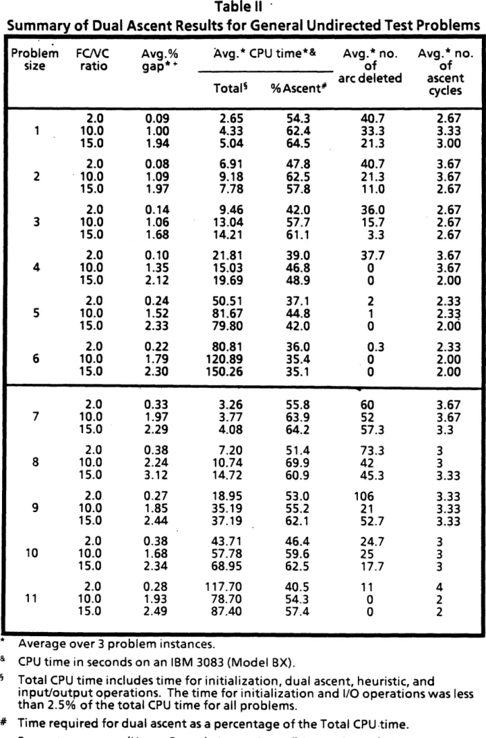
4.1 General Undirected Test Problems: Random, Undirected Networks with Complete Demand and Euclidean Costs
We used the following problem generating program to construct test problems in this category. The network generator first selects the required number of nodes (specified by the user) from a 100 x 100 grid in the plane and generates a random spanning tree over these nodes (to ensure that the problem
is feasible). The required number of remaining arcs are then randomly
k
(i,j), the variable cost c..j is the same for all commodities k and is set equal to the Euclidean length of arc i,j} (rounded to the nearest integer). The fixed charge Fij is some user-specified multiple of the variable cost. All problems have a complete demand pattern, i.e., one unit must be
transported from each node to every other node. Transshipment is permitted at every node.
For our experiments we generated these problems in eleven sizes ranging from 20 nodes, 80 arcs and 380 commodities to 45 nodes, 500 arcs and 1980
commodities. Table I shows the dimensions of the network for each of the
eleven problem sizes. Problems in categories 1 to 6 represent sparse networks
with varying levels of arc densities. Problem sizes 7 to 11, on the other
hand, correspond to complete networks.
For each problem size, we considered three realistic fixed-to-variable cost ratios of 2, 10 and 15; as the fixed charge increases in this range relative to the variable cost, we expect that the problems will become harder to solve. We generated three instances, using different random number seeds,
for each of the 33 problem combinations.
Implementation Details
Our FORTRAN implementation of the composite dual ascent-based algorithm to solve this class of undirected network design problems incorporates the enhancement and the iterative dual ascent scheme based on complementary
slackness violations described in Sections 3.1 and 3.2, as well as a drop-add
heuristic that uses an initial design derived from the dual solution. (The
drop-add method first drops arcs successively as long as the total cost
decreases before initiating the add phase.) The main subroutines in the
program are (i) an "unrestricted" dual ascent routine, (ii) a "restricted" dual ascent routine that takes into account complementary slackness
restrictions, and (iii) the drop-add heuristic procedure. The only problem reduction test that we implemented was the Arc Exclusion method to eliminate arcs {i,j} whose remaining slack s.. exceeds the difference between the
1J
current best upper and lower bounds. Figure 4.1 contains a flowchart showing
the interrelationships between the various segments of the composite program.
- 34
---0 0 00 00 O 0 0 O O O O O O O o N O O O 4 (N en (N OO r- M. ~-. '1 !. o o 0 0 0 o m LA 0 0 V- -1 - q LA O O O 0 0 O 00 0 r1. o % 00C M Q 0 0 D 0 O O e O O CD . 1 - O LA O Ln O LA 0 L r4I N M M en t - (N Mn R LA %A -M 0 L 0