Dynamic scheduling of a multiclass make-to-stock queue

^

*

_Of

-'

O

/

&

&

WORKING

PAPER

ALFRED

P.

SLOAN

SCHOOL

OF

MANAGEMENT

DYNAMIC

SCHEDULING

OF

A

MULTICLASS

MAKE-TO-STOCK

QUEUE

Lawrence

M. Wein

Sloan SchoolofManagment,

MIT

Working

Paper No. 31

13-90-MSA

MASSACHUSETTS

INSTITUTE

OF

TECHNOLOGY

50

MEMORIAL

DRIVE

DYNAMIC

SCHEDULING

OF

A

MULTICLASS

MAKE-TO-STOCK

QUEUE

Lawrence

M. Wein

SloanSchool ofManagment,

MTT

Working

Paper No. 31

13-90-MSA

Wi.l.T.

UBRAh,.

DYNAMIC

SCHEDULING

OF A MULTICLASS MAKE-TO-STOCK

QUEUE

Lawrence

M.

Wein

Sloan School of

Management,

M.I.T.

Abstract

Motivated by make-to-stock production systems,

we

consider a scheduling problem for a single-server queue that can process a variety of different job classes. After jobs

are processed, they enter a finished goods inventory that services customer

demand.

The

scheduling

problem

is to release jobs to the queue

and

decide which job class, if any, to

serve next in order to minimize the long run expected average cost incurred per unit of time, which includes linear costs (which

may

differ by class) for backordering finished goods inventory, holding finished goods inventory,

and

holding

WIP

inventory.

Under

the

heavy traffic condition that the server

must

be busy the great majority of the time in

order to satisfy customer

demand,

the scheduling problem is approximated

by

a

dynamic

control

problem

involving

Brownian

motion.

The

Brownian

control

problem

is solved,

and

its solution is interpreted in terms of the queueing system in order to obtain an effective

scheduling policy.

The

proposed scheduling policy releases jobs to the queue only

when

they are about to begin processing,

and

keeps the server busy as long as the weighted

sum

of the finished goods inventory (where the inventory of each class is weighted

by

its

expected processing time) is not too large.

When

the server is working, priority is given to backlogged classes that areexpensive to backlog

and

haveshort expected processing times,

and

when

there are

no

backlogged jobs, priority is given to jobs that are inexpensive to

hold in finished goods inventory

and

have long expected processing times.

DYNAMIC

SCHEDULING

OF

A

MULTICLASS MAKE-TO-STOCK

QUEUE

Lawrence

M.

Wein

Sloan School of

Management,

M.I.T.

Production facilities are often categorized as

make-

to-ordersystems or make-to-stock systems. In make-to-order systems, the facility produces according to customer requests,

and no

finished goods inventory is kept. In make-to-stock systems, the facility produces

according to aforecast of customer

demand, and

completed jobs enter a finished goods in-ventory,

which

in turn services actual customer

demand.

Due

to increasedglobal

manufac-turing competition, the customer response time (the length oftime between the placement of a customer's order

and

the delivery of the order) required to stay in business is being

reduced,

and

is sometimes smaller than a firm's manufacturing cycle time (the length of time

between

ajob's start of production

and

its completion). In such cases, the facility is

forced to operate (at least partially) as a make-to-stock production system.

The

goal of this paper is to investigate the scheduling

problem

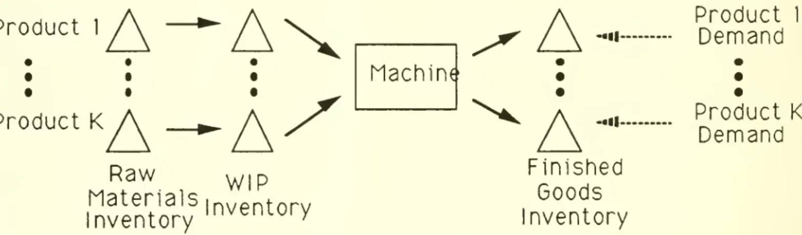
faced by a single machine, make-to-stock production facility in a

dynamic

stochastic environment. This

facility is pictured in Figure 1, where it is

assumed

that there is an

ample

amount

of

raw

material inventory of product k, for k

=

l,...,iv.

The

scheduler decides

when

to release a

raw

product kjob onto the shop floor, at which time thejob

becomes

a unit ofproduct k work-in-process (

WIP)

inventory.

These

decisions will be referred to as release decisions.

There

is a single

machine

that transforms units ofproduct k

WIP

inventory into units of product kfinished goods inventory.

The

machine

is

modeled

as a multiclass queue, in that the

machine

may

work

on only one unit at a time,

and

each product has its

own

general

processing time distribution.

Demand

foreach product can be any arbitrary point process that satisfies a functional central limit

theorem

(forexample, a

compound

Poisson process).

among

K

+

1 options at each point in time: either

work

on a type k product, k

=

1, ...,

K,

or allow the

machine

to sit idle. Preemptive

resume

scheduling is allowed, but as will be

seen later, our

method

of analysis is crude

enough

that our resulting scheduling policy is

independent of the particular assumptions

made

with regard to preemption. There are

no

set-up times incurred

when

switching production

from

one type of product to another.

There

are linear costs incurred per unit of time for backordering finished goods inventory,

holding finished goods inventory,

and

holding

WIP

inventory,

and

these costs

may

differ

by product.

The

scheduling

problem

is to find a release policy

and

a sequencing policy to minimize the long run expected average backorder

and

holding (both

WIP

and

finished goods) cost incurred per unit of time.

Product

1

Product

K

A—

A

Raw

_W)p

hUSintifrl?

Inventory

Inventory

;

Machine

A

A

-•ii-

-.11-Finished

Goods

Inventory

Product

1

Demand

Product K

Demand

Figure

1.

The

Production Facility.

In order to analyze this scheduling problem,

we

have

employed

a

Brownian model

developed by Harrison (1988) that approximates, under so-called heavy traffic conditions,

a

dynamic

scheduling

problem

for a multiclass queueing network by a

dynamic

control

problem

involving

Brownian

motion.

The

heavy traffic conditions

assume

that the server

must be busy

the great majority of the time (for example,

90%

of the time) in order to

satisfy customer

demand

over the long run.

By

solving a reformulation of the

Brownian

control

problem

and

interpreting the solution in terms of the original queueing system, a

variety of seemingly intractable scheduling problems have been analyzed; see, for

exam-ple, Harrison

and

Wein

(1989),

Wein

(1989a,1989b),

and

Laws

and Louth

(1988). In this

paper,

we

alter Harrison's

model

to

accommodate

afinished goods inventory that services customer

demand, and

approximate a multiclass make-to-order queueing system

schedul-ing

problem

by a

dynamic

control problem involving

Brownian

motion.

A

closed form solution to the workload formulation ofthe control problem is obtained,

and

this solution

is interpreted in terms of the original production/inventory system in order to obtain an effective scheduling policy.

Not

surprisingly, the proposed release policy releases a

raw

unit ofproduct k to the

shop only

when

the scheduler decides to process a type k unit,

and

thus no

WIP

inventory

is held.

Although

the release decisions appear to be superfluous in our model, the

main

reason they are included is to maintain consistency with Harrison's original model, which

considers a general queueing network with controllable inputs

and dynamic

scheduling

capability.

By

appending

the customer

demand

process

and

finished goods inventory to

Harrison'smodel, one canformulate acontrol

problem

(job release

and

priority sequencing)

for a very general make-to-stock queueing network.

The

proposed sequencing policy dynamically tracks the weighted inventory process, which is the weighted (by the

mean

processing times)

sum

ofthe finished goods inventory

levels (which can

be

positive or negative) ofeach product.

Whenever

the weighted

inven-tory process is below a certain critical value, then the

machine

stays busy; otherwise, it is

idle.

When

the

machine

is busy, it employs a

dynamic

sequencing policy that is

somewhat

reminiscent of the so-called c\i rule that minimizes the weighted average cycle time in a

conventional multiclass queue. In the c/x rule, c_k is the holding cost for class k jobs in

queue

and

//* is the service rate,

and

the rule gives priority to larger values of the index

Ckfik- In our setting, let the backorder cost for type k products be 6*, the finished goods

inventoryholding cost be denoted by h_k,

and

the service ratebe/x*-

Among

the job classes

largest value of the index 6*^*- If

no

job classes are backlogged, then priority is given to

the class with the smallest value ofthe index h^Hk-

A

simulation experiment is performed

with

two

numerical examples,

and

the proposed policy is

compared

to the conventional scheduling policy of releasing jobs as above, keeping the

machine

busy

whenever

the total

(unweighted) inventory process is below a critical value,

and

dynamically awarding priority to the class with the smallest finished goods inventory level.

The

proposed policy reduces the total cost

by 14.9%

and 23.2%

relative to the conventional policy in the two numerical examples.

An

important implication ofthe balanced heavy loading conditions

assumed

in Harri-son's

Brownian

network

model

is that, in the heavy traffic limit represented by the

Brow-nian model, any stations in the original queueing network that are not

among

the

most

heavily loaded will simply vanish. This has been provenfor

some

single-type queueing net-works (see

Johnson

1983

and

Chen

and

Mandelbaum

1989),

and

justifies the procedure of

eliminating allnon-bottleneck stations

when

performing the

Brownian

analysis. Therefore,

our scheduling policy applies to any make-to-stock production system with one bottleneck workstation that does not allow jobs to visit this station

more

than once.

The

remainderofthis paper isorganized asfollows.

The

relevant literatureis reviewed

in Section 1, the queueing system scheduling

problem

is defined in Section 2,

and

the

corresponding

Brownian

controlproblem isgivenin Section3.

The

problemis reformulated

in terms of workloads in Section 4,

and

the workload formulation is solved in Sections 5 through 9.

The

solution is interpreted in Section 10,

and

a simulation experiment

is performed in Section 11 to demonstrate its effectiveness. Section 12 contains

some

concluding remarks.

This section concludes with the probabilistic formalisms that will be adopted in this

paper.

When

we

say that

X

is a

A'—

dimensional (/i,E)

Brownian

motion (readers are

referred to Karatxas

and

Shreve 1988 for a definition), it is

assumed

there is a given (J),F,

F

t,

X,

P

z),

where

(ft,F) is a measurable space,

X

=

X(lj) is a measurable

mapping

of 0, into

C(R

K

), which is the space of continuous functions

on

R

K

,

F

t

=

a(X(s),s

<

t)

is the filtration generated by

X,

and

P

z is a family of probability measures on

Q

such

that the process {X(t),t

>

0} is a

Brownian motion

with drift fi, covariance matrix E,

and

initial state x under

P

z. Let

E

_x be the expectation operator associated with

P

_z. If

Y

=

{Y(t),t

>

0} is a process that is

F

_t-measurable for all t

>

0, then

we

say that the

process

Y

is non-anticipating with respect to the

Brownian

motion

X

.

More

generally,

we

will say that one process

Y

is non-anticipating with respect to another process

X

when

Y

is adapted to the coarsest filtration with respect to which

X

is adapted.

1.

Relevant

Literature

The

problem

posed in thispaper istodynamically schedule a multiclass make-to-stock queue,

which

represents a multi-product, single machine, production/inventory system. Notice that the conventional multiclassqueue (wherejobsarrive

randomly

and

thenexit the

system after service is completed) corresponds to a multi-product, single machine,

make-to-orderfacility.

Although

the

problem

ofminimizing the

number

ofjobs in a conventional

multiclass queue has been thoroughly

examined

(see, forexample,

Klimov

1974), there are

no

studies that explicitly analyze the multiclassmake-to-stock queue. However, there have been several studies analyzing single-machine production/inventory systems with

random

demand.

Gavish

and

Graves (1977)

and

Graves

and

Keilson (1981) consider the single-product case with deterministic processing times

and

set-up costs. Here the scheduling

problem

is to decide

when

to start

and

stop the machine. Graves (1980) attempts to generalize these results to the multi-product case by considering a periodic review policy

and

introducing the notion of a composite product.

Bemelmans

and Wijngaard

(1982)

also aggregate the products in a single-machine, multi-product problem, although their production

model

is different than a standard queueing model, in that the

machine

is

allowed to

work on

several products simultaneously.

The

paper that is

most

closely related to ours is probably

Zheng and

Zipkin (1990),

who

analyze a production/inventory system that produces

two

distinct products.

The

production system is modelled as a single server queue with exponential processing times,

the customer

demand

for each product is a Poisson process,

and

an (S

—

_1,5) policy is

used to trigger ordersforeachproduct to theproduction system.

They

analyze this system under

two

different sequencing policies:

FCFS,

and

serve the product that has the lower inventory level. Theirqueueing theoretic analysis revealsthat thelatterpolicy outperforms

FCFS.

There

is also a substantial literature

on

dynamic

lot-sizing problems, but these

mod-els (except for the presence ofset-up times) are

more

restrictive than a standard queueing model. Readers are referred to the survey paper of Graves (1981) for

more

on these

prob-lems.

He

reviews scheduling problems for both make-to-order

and

make-to-stock systems,

and

refers to these systems as

open

shops

and

closed shops, respectively.

Our

consideration ofqueueing

and

inventory aspects in asingle

model

is not new. In

fact, the analysis

and

design of such systems have been the subject of

much

recent work;

see, for example, Williams (1984), Bertrand (1985), Zipkin (1986),

Karmarkar

(1987),

Cohen

and

Lee (1988), Altiok (1989),

and

Mitra

and

Mitrani (1988). In particular, it

was

the paper

by

Zipkin (1986) that partially stimulatedthis analysis. Finally, the heavy traffic

theory for queueing systems underlying this

Brownian

model

offers a partial justification

for the direct

modeling

ofan inventory storage system by a diffusion process, both in past

(see, for example, Bather 1966,

Puterman

1975,

and

Browne

and

Zipkin 1989)

and

future research efforts.

2.

The

Scheduling

Problem

Consider a single server that can serve

K

different classes of jobs.

We

refer to the

entities populatingthe queueingsystem asjobs rather than customers, so as not to confuse

them

with the actual customer

demand.

In terms ofthe production/inventory system, the server is the machine, each job class corresponds to a type of product,

and

each job is a

unit of a particular product. Class k jobs have a general service time distribution with

finite

mean

m*

and

variance s\, for k

=

1,...,K.

The

service times (or processing times)

for class k are equivalently characterized

by

therenewal process S*(r), whichis the

number

of class k service completions

up

to time i if the server were continuously serving class k

jobs in the interval [0,i].

Adopting

conventional terminology,

we

will refer to //*

=

m^

1

as the service rate of class k jobs.

For each class k

=

1,...,A", there is an independent

demand

process -Djt(r), which is

the

number

ofclass k units

demanded

up

to time t. For

now we

will

assume

that Dk(t) is

a renewal process,

and

that interarrival times of this

demand

process have

mean

A^

and

variance a?.

As

will be seen in the next section, this assumption can be relaxed,

and

all

that is required is that £>* satisfy a functional central limit

theorem

(FCLT).

There

are

two

types of decisions in the scheduling problem,

and

these decisions take the

form

of cumulative control processes. Let the reiease process Nk(t) be the

number

of class k jobs released to the machine's queue in [0,r]. Let the allocation process Tjt(i)

be the cumulative

amount

of time that the server devotes to serving class k jobs in [0,r].

Then

the vectors TV

=

(7V

fc)

and

T =

(7*) represent the release

and

sequencing policies,

respectively. Let Qk(t) be the

number

of class k jobs in the queue or in service at time

t,

and

let Zk(t) be the

number

of units (possibly negative) of class k jobs in the finished goods inventory.

The

vectors

Q

=

_(Qk)

and

Z

=

(Z*) will be called the queue length process

and

inventory process, respectively. If

we

assume

that _Q(0)

=

Z(0)

=

0, then it

follows that for k

=

1, ...,

K

and

t

>

0,

Qk(t)=N

k

(t)-Sk(T

k (t)),

and

(2.1)

Zk(t)=Sk(T

k(t))-Dk(t). (2.2)

Furthermore, if

we

define the cumulativeidlenessprocess I(t) to be the cumulative

amount

of time the server is idle in [0, t], then

K

I(t)=t~Y

t

As

in Harrison (1988), a scheduling policy

(N,T)

must

satisfy

T

is continuous with T(0)

=

0, (2.4)

N

and

T

are nondecreasing

and

JV(0)

=

0, (25)

N

and

T

are nonanticipating with respect to _{Q, (26)}

J is nondecreasing with ₁₍₀₎

=

0,

and

(2.7)

Q(t)

>

for all t

>

0, (2.8)

where

constraint (2.6) implies that the scheduler cannot observe future

demands

or service times.

Now

define the cost function ck for k

=

1,...,A', by

<*(*)=(?'*'

*

X

"°

;

(2.9)

v

' _{\ h}

kx, ifx

>

0, v ;

where

b^ represents the backorder cost for class k jobs,

and

/i* is the finished goods inventory holding cost for class k jobs. It willbe

assumed

that 6*

>

hk

>

0,for k

=

1, ...,

K,

in order to guarantee an interesting problem. Since the optimal

WIP

inventory levels will be zero,

we

will omit different

WIP

holding costs for eachjob class, in order to limit the

amount

of notation used. Thus, the scheduling

problem

is to choose a policy

(N,T)

to

T

K

K

minlimsupi£:[/

_f]

_Q

k{i)

+ f]

c_k

(Z

k(t))dt] (2.10)

T-oo

J _Jo

k=1 k=1

subject to constraints (2.1)-(2.8).

3.

The

Limiting

Control

Problem

In this section, a

Brownian

approximation to the control

problem

(2.1)-(2.8), (2.10)

will be developed.

We

follow the approach taken in Sections 3 through 5 of Harrison

(1988), which approximates a system that in

most

respects is

more

complex

than the

one considered here.

Only

the basics of the approximation are provided,

and

readers are

referred to Harrison (1988) for a

more

detailed presentation

and

justification.

The

first

step in the approximation is to define a collection of centeredprocesses. _{Let p}k

=

^k /p- k

be the proportion of time that

must

be devoted to serving class k jobs in order to satisfy

the average

demand.

The

traffic intensity of the system, defined by _p

=

_Yik=\ P*> 1S t^ie

average server utilization required to satisfy average

demand.

Define

a

k

=

pk/p to to be

the proportion of the server's busy time that

would

be devoted to serving class k jobs if the server

met

average

demand

exactly. For k

=

1,...,K

and

t

>

0, define the centered

processes

Y

k (t)

=

a

k

t-T

k (t), (3.1)

9k(t)

=

\kt

-

N

_{k (t),}

and

(3.2)

n_k(t)

=

S

k

(t)-p

kt. (3.3)

Notice that

Y

=

(Y

k)

and

8

=

(6k) are control processes

and

are centered around

the nominal allocation rates

and

nominal input rates, respectively. Finally, define the

IK—

dimensional process £ by

Ck(t)

=

(A*

-

fik

a

k)t

-

Vk(T

k(t)), for k

=

1,...,A',

and

t

>

0,

and

(3.4) (

K

+k(t)

=

(»kc*k

-\k)t

+

Vk(T

k (t))

-

D

k (t)

+

\kt, for k

=

1,...,

K, and

t

>

0.(3.5)

Then

it follows

from

(2.1)-(2.3), respectively, that

Qk(t)

=

(k(t)

+

fik

Y

k(t)

-

6k(t), for k

=

1, ...,

K, and

t

>

0, (3.6)

Z

k(t)

=

CK+k(t)-fikY

k (t), forfc

=

l,...,A-,

and

t

>

0,

and

(3.7)

K

I(t)

=

J2

Y

k(t_),

fort>0.

(3.8)

As

inHarrison (1988), thekey tothe approximationisto replacetheallocation process

T

k(t) in (3.4)-(3.5) by its nominal allocation rate

a

kt. Readers are referred to Section 5 of Harrison (1988) for an informal defense of this substitution. This replacement causes the

2A—

dimensional process £* in (3.4)-(3.5) to be replaced by \k, where, for t

>

_0,

Xk(t)

-

(A*

-

Hk<*k)t

-

Vk(

a

kt), for k

=

1,...,A',

and

(3.9) CK+k(t)

=

(nkC*k-Xk)t

+

rik(<*kt)-Dk (t)

+

\kt, for fc

=

l,...,#. (3.10)

We

will also replace £ by

x

in the definitions of the queue length process

Q

and

inventory process

Z

in (3.6)-(3.7).

The

final step in the

Brownian

approximation is to rescale the basic processes under

heavy

traffic conditions, which

assume

theexistence ofalarge integer

n

that approximately

equals (1

—

p)~2.

A

representative

example

is to choose

n

=

100 if the traffic intensity

p

=

.9. Using the system parameter n,

we

define the scaled processes (the

same

symbols are used on both sides of equations (3.11)-(3.13) in orderto reduce the notational burden)

Q

k(t)

=

3*(g*) for Jt

=

l,...,A',

and

t

>

_{0, (3.11)}

y/n

Z

k

(t)=

Z

, for

k=

1,...,A',

and

t

>

0, (3.12)

Y

k(t)

= ¥±^l,

for

k=

1,...,A,

and

r

>

0, (3.13)

V"

^(nt)

gfc(<)

=

V

, for Jfc

=

1,...,A,

and

t

>

0,

and

(3.14) y/n

/(<)

=

-i^2,

for Jfc

=

l,...,A,

and

<

>

0, (3.15)

and

the

Brownian

approximation is essentially obtained by letting the parameter n

—

oo.

The

processes _Q,Z, K,#,

and

J

now

represent limiting scaled processes,

and

will still be

referred tosimplyas thequeue length, inventory, allocation, release,

and

idleness processes.

The

process \ in (3.9)-(3.10) also needs to be rescaled. Define _{x* by}

x

«(i)

=

2l4^1

for k

=

1,...,2A,

and

t

>

0. (3.16)

y/n

Then

a straightforward application of the functional central limit

theorem

for renewal processes

and

the

random

time change theorem (see Section 17 of Billingsley) implies that

X

nk

^X

k,

for*

=

l,...,A, (3.17)

where =>• denotes

weak

convergence,

and

X\,...,Xk are independent

Brownian

motion

processes with drift y/n(\k

—

fik

a

k)

and

variance

a

k^i\s 2

k. Similarly, applying the above

two

theorems

and

the continuous

mapping

theorem (Billingsley,

Theorem

5.1),

we

have

Xnk

^X

k,

for*

=

tf

+

l,..,2tf, (3.18)

where

Xk+\,...,X

2

k

are independent

Brownian

motion processes with drift

—^/n(X

k

—

fik

Q

k)

and

variance

a

kfj. 3 ks 2 k

+

\ 3 ka. 2

k. Notice that any

demand

process satisfying afunctional

central limit

theorem

can be incorporated into our model.

Thus

characteristics of actual customer

demand,

such asbatch arrivals

and

dependencies acrossproducts (e.g., customers arrivingwith

demands

forseveral products) can be modeled; see Section6 of

Reiman

(1984)

for

more

details.

We

are

now

in a position to state the limiting control problem, which is to choose

K—

dimensional

RCLL

(right continuous with left limits) processes

Y

and

8 to

T

K

K

min

limsup-£

r_[/

VQ

t (f)

+

Vc*(Z*(t))«ft] (3.19)

r-oo

l _Jo

k=1 t=1

subject to

_Q

k(t)

=

X

k(t)

+

n

k

Y

k

(t)-6

k (t), for fc

=

l,...,A',

and

t

>

0, (3.20)

Z

k(t)

=

X

K+k

(t)-fik

Y

k(t)

fovk

=

l,...,K,

and

t

>

0, (3.21)

K

U(t)

=

Yl

Y

k(t)iovt>0,

(3.22)

fc=i

Q(t)

>

for all*

>

0, (3.23)

U

is nondecreasing with U(0)

=

0,

and

(3.24)

9

and

Y

are nonanticipating with respect to

X.

(3.25)

4.

The Workload

Formulation

The

basicsystem stateequations (3.20)

and

(3.21) areintermsofthe

number

ofjobsin

WIP

inventory

and

finished goods inventory, respectively. In this section,

we

reformulate the limiting control

problem

(3.19)-(3.25) in terms of workloads,

meaning

that the

two

inventories will

now

be expresses in terms of the

amount

of

work embodied

in them. First

define the one-dimensional

Brownian

motion

B\

by

K

B

1(t)

=

J2

m

kX

k {t),

t>0,

(4.1)

t=i

so that

B\

has drift \/™_]Ct=i

m

*(^*~

Hk<*k)

—

\/^(p

—

^)

<

and

variance p

-1

5Zfc=i ^*5

Jt-Similarly, let the one-dimensional

Brownian

motion

B

₂ be defined by

K

B

2(t)

= Y,

m

k

X

K

+k(t), t

>

0, (4.2)

*=i

with drift y/n(l

—

_p)

_>

and

variance />

-1

(X)fc=i ^*5*)

+

Ylk=i P\^*a\-

The

workload

formulation of the limiting control

problem

(3.19)-(3.25) is to choose the

A'—

dimensional processes

Q,

Z,

and

#,

and

the one-dimensional process

U

to

T

K

K

min

limsup-£

r _[/

V

Q

k(t)

+

V

c*(Z*(t))<ft] (4-3)

subject to

^2m

k

Q

k (t)

+

^2m

kek(t)

=

Bi(t)

+

U(t), for <

>

0, (4.4)

k=l k=l

K

Y

J

™

k

Z

k {t)

=

B

₂{t)-U{t), for t

>

0, (4.5) *=i Q(<)

>

for all*

>

0, (4.6)

U

is nondecreasing with U(0)

=

0,

and

(4-7)

Q,Z,U,

and

6 are nonanticipating with respect to A'. _(4-8)

Let (Y, 0) be a feasible solution to the limiting control

problem

(3.19)-(3.25) if (Y,9)

satisfies (3.20)-(3.25),

and

let _(Q, Z, U,8) beafeasiblesolution tothe workloadformulation

(4.3)-(4.8) if_(Q,Z,U,6) satisfies (4.4)-(4.8).

Then

problems (3.19)-(3.25)

and

(4.3)-(4.8)are

equivalent formulations, as can be seen

from

the following proposition.

Proposition

1.

Every

feasiblepolicy (Y,8) for the limiting control

problem

yields a

corresponding feasible policy

(Q,Z,U,d)

for the workload formulation,

and

every feasible

policy (Q,Z, U,6) for the workloadformulationyields a correspondingfeasiblepolicy _{(Y, 9)} for the limiting control problem.

Proof.

Let (Y,8) be any feasible policy for the limiting control problem,

and

define Q,Z,

and

U

by

Q

k(t)

=

X

k (i)

+

HkY

k(t)

-

6k (t), for k

=

1, ...,A',

and

t

>

0, (4.9)

Z

k(t)

=

X

_K+k

(t)

-

fik

Y

k(t), for k

=

l,...,K,

and

t>0,

and

(4.10)

K

[7(r)

=

^r

it(r)forr

>0.

(4.11)

Then

(3.25)

and

(4.9)-(4.11) imply that (4.8) holds, (3.22), (3.24),

and

(4.11) imply (4.7),

and

(3.20), (3.23),

and

(4.9) imply (4.6). Also, for t

>

0,

K

K

K

K

^m

iQ,(r)

=

^m

Jt

X

t

(0

+

^m^

Jt

yi(r)-^m^

t(0, by (4.9), (4.12)

Jt=i *=i Jt=i t=i

K

=

B

1(t)

+

V{t)-Y,

m

kh(t)1

by

(4.1)

and

(4.11), (4.13)

fc=i

and

so (4.4) holds. Similarly,

K

K

K

J2

m

kZ

k(t)

=

Y

/

m

k

X

K+k

(t)-Y

/

m

kfik

Y

k(t),

by

(4.10), (4.14) k=l k=l fc=l

=

B

2 {t)

-

U(t), by (4.2)

and

(4.11), (4.15)

and

so (4.5) holds.

Thus

(Q,Z,U,6)

is a feasible solution to the workload formulation.

Reversing the argument, let us suppose that

(Q,Z,U,6)

is a feasible policy for the

workload formulation,

and

define

Y

by

Y

k(t)

=

m

_k

X

_K+k

{t)

-

m

_k

Z

_{k (t),} for k

=

l,...,K,

and

t

>

0. (4.16)

Then

(4.8)

and

(4.16) imply (3.25), (4.16) implies (3.21),

and

K

K

K

£n(0

=

£

m

_***+*(*)-E

m

*

Z

*(')'

by

(4.16), (4.17) k=\ k=\ *=i

K

=

B

2

(0-^m

fc

Z

fc(0,

by

(4.2), (4.18)

=

U(t),

by

(4.5), (4.19)

and

so (3.22) holds,

and

(4.7) implies (3.24). Finally, for k

=

1,...,A',

and

t

>

_0, (4.16)

implies that

X

k(t)

+

n

k

Y

k (t)

-

6k(t)

=

X

k (t)

+

fik

m

k

X

K+k

(t)

-

fik

m

k

Z

k(t)

-

6k(t), (4.19)

=

X

k(t)

+

X

K

+k(t)

-

Z

k{t)

-

6k(t), (4.20)

=

Qk(i), by (4.9)

and

(4.10), (4.21)

and

thus (3.20) holds,

and

(4.6) implies (3.23). Thus, (Y,9) is a feasible solution to the

limiting control problem. _|

The

next four sections are devoted to solving the workload formulation.

Not

only is the workload formulation easier to solve than the limiting control problem, but its solution

is also easier to interpret in terms oftheoriginal queueing system, as will be seen in Section

10.

5.

The

Three

Step

Solution

Procedure

The

workload formulation (4.3)-(4.8) will be solved in three steps. In the first step,

which

is carried out in this section, the optimal control processes

Q

and

6 are found in terms of the control process

Z

.

The

second step solves for the optimal control process

Z

in terms of the control process

U

,

and

the third step derives the optimal control process

U.

The

first step is

embodied

in the following proposition.

Proposition

2. Let (Z*

,U*,Q*

,0*) denote the optimal solution to the workload

formulation (4.3)-(4.8).

Then

for k

=

1,...,AT,

and

t

>

0,

Ql(t)

=

0,

and

(5.1)

et(t)

=

X

k(t)

+

X

K+k

{i)-Zt(t). (5.2)

Proof.

Let

Z

and

U

be any pair of processes satisfying (4.5), (4.7),

and

(4.8).

Then

the pair of processes defined by Qk{t)

=

for k

=

1,...,

K

and

t

>

0,

and

9k(t)=Xk(t)

+

X

K

+k(t)-Z

k (t), for fc

=

l,...,#,

and*>0,

(5.3)

satisfy (4.4)

and

(4.6). Moreover,

_£)f

₌₁

Q

k(t)

=

for all t

>

0,

and

thus

Q

and

offer

a lower

bound

on

the objective function value in (5.3). Since this

argument

holds for any pair of processes

Z

and

U

satisfying (4.5), (4.7),

and

(4.8), it

must

hold for the optimal

processes

Z*

and

U*, thereby completing the proof. |

The

workload

formulation has

now

been reduced to choosing the nonanticipating,

RCLL

processes

Z

and

U

to 1 r

T

K

min

limsup-£

r[/

Vc*(Z

t(0)<ft] (5-4)

T-oo

T

J

_f^

subject to (4.5)

and

(4.7).

6.

Solving

for

Z

in

Terms

of

U

The

second step of the three step procedure is performed in this section.

Suppose

we

are given a process

U

that satisfies constraints (4.7)-(4.8). Then, by Proposition 2, the

optimal solution

Z

can be derived by solving the following mathematical

program

at each time t: choose Zi(t),...,Zx(t) to

K

min

£c*(Z

fc(0) (6-1)

K

subject to

Y,

m

kZk{t)

=

B

2(t)

-

U(t). (6.2)

Notice that, at time r, the right side of (6.2) is

known,

since the value of

B

2(t) can be observed,

and

it is

assumed

that U(t) isgiven. Let us define theone-dimensional weighted

inventoryprocess

W

by

W(t)

=

B

2(t)

-

U(t), for t

>

0. (6.3) 15

From

(6.2)-(6.3), the process

W

is interpreted as a weighted

sum

of the finished goods

inventory for each product,

where

the weight is the

mean

processing time for the product.

By

the definition of the cost function c* in (2.9), the solution to problem (6.1)-(6.2) can be derived by solving 2h linear programs.

Each

of these LP's are subject to the constraint

K

Y,mkZ

k(t)

=

W(t), (6.4)

k=i

and

each of the LP's corresponds to one of the 1

K

combinations of each

component

of

Z

constrained to be nonnegative or nonpositive, thus leading to a linear cost structure. For example, if

K

=

2, the four LP's are to minimize

—

b\Z\(t)

—

b2

Z

2(t) subject to (6.4)

and

Z

1(t),Z2(t)

<

0; minimize /iiZi(i)

+

h2

Z

2(t) subject to (6.4)

and

Z

x{t),Z2{t)

>

0;

minimize

—

b\Z\{t)

+

h2

Z

2(t) subject to (6.4)

and

Z\{t)

<

0,Z

2(t)

>

0;

and

minimize

hiZi(t)

- hZ^t)

subject to (6.4)

and

Z

x(t)

>

0,Z

2(i)

<

0.

The

solution to (6.1)-(6.2) is

then derived

from

the

LP

that achieves the

minimum

objective function valuefrom

among

the 2

K

LP's.

Analyzed

in this way,

we

can find a simple closed

form

solution to (6.1)-(6.2) for all

values of W(t).

Without

loss of generality, define the indices j

and

/ by

min

=

—

—

and

(6.5)

i<k<K

rrik rrij

min

=

—

,

(6-6)

\<k<K

rrik ttii

where

it is possible for j

=

/.

Then

the optimal solution Z*(t) to (6.1)-(6.2) is

f

mil

if k

=

;

and W(t)

>

0;

W)

={

mk

~

(6-7) I 0, if k

±

j

and

W(t)

>

0.

and

( Ell! if Jt

=

/

and W(t)

<

0;

ZUt)

=

I mk (6.8) I 0, if k 5* /

and

W(t)

<

0.

Notice that the optimal control process

Z*

is expressed in terms of the control process

U

via (6.3).

7.

The

Resulting

Control

Problem

Proposition 2

and

solution (6.7)-(6.8) can be used to reducethe workload formulation

to a

problem

of choosing the optimal control process U. Referring back to (6.5)-(6.6),

let us define h

=

hj/m.j

and

6

=

b//mj. Then, by (2.9)

and

(6.5)-(6.8), the optimal cost

function ct(Z£(r)) is given by f(W(t)),

where

f hx, if x

>

0;

«*>

=

_{

_-K

_**

_<o.

(71)

Thus, f(x) is a piecewise linear, continuous, convex function that achieves a

minimum

of

zero at x

—

0.

Define a policy to be a nondecreasing

RCLL

process

U

such that

U

is nonanticipating

with respect to

B

2,

E

_z[U(t)] is finite for each r

>

and

each initial state

5

2(0)

=

x,

and

£7(0)

=

0.

Then

the resulting

Brownian

control

problem

is to find a policy

U

to

min limsupif?

r

_[/

f(W(t))dt] (7.2)

subject to

W{t)

=

B

2(t)

-

U(t) for t

>

0. (7.3)

Although

U

is nonanticipating with respect to

X

in the workload formulation, it is clear

that

U

onlyhas tobenonanticipatingwithrespect to

B

2.

The

next

two

sectionsaredevoted

to solving

problem

(7.2)-(7.3), which is a one-dimensional singular control

problem

with a long run average cost criterion.

The

term "singular" refers to the fact that the state of the

controlled process

W

can be instantaneously changed

by

the controller and, as a result,

the optimal control process

U

is continuous but singular (i.e., the set of time points at which

U

increases has

measure

zero). Various one-dimensional singular control problems with a long run average cost criterion have been studied by, for example, Karatzas (1983),

Robin

(1983), Menaldi

and Robin

(1984), Taksar (1985),

and

Wein

(1989a).

8.

A

Candidate

Policy

In this section, a candidate policy

U

toproblem (7.2)-(7.3) is derived. Recall that the

Brownian motion

process

B

₂ appearing in (7.3) has drift y/n(l

—

_p)

>

0, which

we

denote

by /i,

and

variance _p

-1

(£2jt=i ^*5*)

+

]Ct=i P*^*a/t> which is denoted by a

2

. Given the

positive drift

and

the nature of the cost function f(x) in (7.1), it is natural to consider a policy that keeps the controlled process

W

in the interval (

—

00,B] while exerting a

minimum

amount

of control,

where

B

is a barrier to be calculated below.

The

controlled

process

W

under such a policy is referred to as a reflected (or regulated)

Brownian

motion

(abbreviated

by

RBM;

see Harrison 1985 for a detailed development),

and

the control

functional

U

is the local time of

W

at the point B. In particular, the control policy

U

with barrier

B

is defined by

U(t)=

sup [B₂

(s)-B]

+, for

t>0.

(8.1)

0<s<t

The

following proposition concerning a one-dimensional

RBM

is needed. See Chapter 1 of Harrison (1985) for a derivation of (8.2)-(8.3),

and

see

Theorem

7.2 of

Abate and Whitt

(1987) for a proof of (8.4).

Proposition

3.

Suppose

2?₂ is a (p.,

a

2

)

Brownian

motion,

U

is defined as in (8.1),

and

thus

W

=

Bj

—

U

is a

RBM

on

(—

00,B].

Then

W

has an exponential steady state distribution with density function

p(x)

=

veu(l-B), for

x<B,

(8.2)

where

»-H.

(8-3)

<y-Furthermore, for each starting state x

<

B, there exists a constant

K

such that

E

x

[W

2

(t)}

<K

for all t

>

0. (8.4)

Thus, if

we

restrict ourselves to the class of policies in (8.1), then problem (7.2)-(7.3)

becomes

one offinding

B

to minimize

F(B), where

B

/0

,B bxue"(z-B)

dx+

/

hxve

v{z-B) dx. -oo JO

Proposition

4.

The

solution to (8.5) is

(8.5) fUH

a--gi.(i

+

J).

(8.6)

*tiT)-Ur-^Ia(l

+

_j[). (8.7)

Proof.

Integrating (8.5) by parts

and

canceling terms gives

F(B)

=

-e-"

B

+

hB-

-(1

-

e-"

B

). (8.8)

Setting

F'(B)

=

yields (8.6). Also,

F"{B)

=

u(h

+

b)e-vB

>

0, (8.9)

so

F(B)

is convex

and

B*

minimizes

F(B).

Since e~

vB'

=

_h/(h

+

6), it follows

from

(8.8)

that

'<*>-&T»h"

r

-r(

1

-s?»)-

ur

" (810)

9.

Proof

of

Optimality

The

following

theorem

provides sufficient conditions for the candidate policy from

Section 8 to be an optimal policy for

problem

(7.2)-(7.3). Let

^^Vj

+

T

(91)

2

dx

2

_ox

19

be the infinitesimalgeneratorof the

Brownian motion

B

2.

As

is usual in control problems

with long run average cost criterion, the _{gain g represents the}

minimal

average cost of

problem

(7.2)-(7.3)

and

the potential function

V(x)

represents the cost incurred under

the optimal policy

when

the initial state of the controlled process

W

is x

minus

the cost

incurred incurred under theoptimal policy

when

the initial state is in

some

reference state,

which

in this case is B.

Theorem

5.

Suppose (g,V(x),B)

satisfy

TV(x)

+

f{x)

-g>0

for x

>

B, (9.2)

TV(x)

+

f(x)

-

g

=

for x

<

B, (9.3)

V'(x)

<

0, for x

<

B,

and

(9.4)

V'(x)

=

0, for x

>

B, (9.5)

and

there exist constants A'i,A'2,

and

A'3 such that

0<V(x)<K

Q -\-K1x

+

K

2x 2

for all x. (9.6)

Let

U(t)=

sup [B₂

(s)-B)

+,

forr>0.

(9.7)

o<»<«

and

suppose

1 r

T

min

limsup-£[/

f(B

2(t)

+

U(t))dt]

=

g. (9.8)

T—

00 J- _Jo

Then

U

is the solution to

problem

(7.2)-(7.3)

and

g is the

minimal

average cost.

The

proofconsists of

two

main

parts,

and

the first part is posed as a

lemma,

where a solution isfound to theoptimalityequations (9.2)-(9.5).

The

basic condition for optimality

can be written in the form

rmn{TV{x)

-

f(x)

+

g,

-V'(x)}

=

0, (9.9)

which is implied by (9.2)-(9.5). This equation can be heuristically derived by considering

the optimality equations forthe corresponding discounted

problem

(see, for example,

Har-rison

and

Taksar 1983)

and

letting the discount rate tend tozero (see,for example, Taksar 1985).

Lemma

6. (g*,V*(x),

B*)

satisfy (9.2)-(9.6),

and

(9.8), where

ha

2 , . 6 X °

=

l7

ln(1+

';) •

ir-gKl

+

_|).

and

ifx

>

B;

(y)dy, ifx

<

B,

where

V'(x)=

i

H

₁

+

I)

"

T

+

W

~

^gJ^e-*"-/'',

ifx

€

[0,5]; ifx

>

B. ( ho 2. ho*

w

(9.10) (9.11) (9.12) (9.13)

Proof.

1°. Notice that

B*

and

g* are the candidate policy

and

candidate

minimum

cost function, respectively,

from

Proposition 4,

and

thus (9.8) is satisfied.

We

start

by

substituting g*

and

B*

into (9.3)

and

solving

\v'\x)

+

/zV'(z)

+

/(*)

-

—-

ln(l

+

_^)

=

0,

for V'(x),

which

yields

V'(«)

=

_^4

M

1

+

_T)

+ Ce-"

"

^2e ~"Z

f

f(vV"

d_V> for x

_£

B

* '

w

_2/i2 v _{AT cr}2 y.oo

where

C

is a constant. Setting V*'(B*)

=

in (9.15) gives

/i<72 , , 6.

Ch

°

=

rjlnl

+

T

+TTL

2/i2 v h' h

+

b

-^^[-b

L^

dv+h

f^

vd

\

(9.14) (9.15) (9.16) 21

Integrating by parts yields

ha

, , b_s

Ch

2 , h _x

2/i2 v /i

y

/i

+

6 a2Kh

+

b'

—

+

1/ »/* (9.17) Since e"°

=

(h

+

b)/h,

we

have

ha*

Ch

ha

7

°--^^

l+

J

+

Tr

b

-^

1+

fr

(9.18) so that

C

=

0. Thus, V*'(x)

=

2^

2 ln(l

+

-)

+

—

e""1 / frye"My, for

x<0,

(9.19)

which

yields the top part of (9.13),

and

ha

V-(,)-_,h(l + -)--

_I.-

_-6

_/

_ye"v

_dy+h

_I

_ye"5

J—

oo JO

dy ,

forx€

[0,B*], (9.20)

which

yields the

bottom

part of (9.13). Setting V*'(x)

=

for x

>

B*

implies (9.5),

and

defining

V*(x)

as in (9.12) implies (9.3).

2°. In order to verify (9.2), notice that for i

>

B*

, (9.5) implies

TV*(x)

=

0,

and

thus

TV*(x)

+

f(x)-g*

=

hx-hB*

>0.

(9.21)

3°. Condition (9.4) will

now

be verified. First, notice that

ha

ba'

^'(°)-ctM1

_2/z2 "~" v~

+

'

t)-o3

h'

2^

ha

2

"

"

V

<o,

ln(l

+

-)--(9.22) (9.23) (9.24)

since ln(l

+

x)

<

x. Since

V*"(x)

=

(6//i)

>

for x

<

0, it follows that V*'(x)

<

for x

<

0. For x

6(0,5*),

V*"(x)

=

--

+ (^-^)e-

2

^/"

2 ,

and

(9.25) 22

V»'(x)

= (^±^)(-^)e-

2"'/"

2

<

0. (9.26)

/x

a

1

Since

V*"(x)

gives a value of zero at x

=

B"

in (9.25), (9.26) implies that V*"(x)

>

for x € (0,i?*). Condition (9.4) follows by the continuity of V*'(x)

and

the fact that

V*'(B*)

=

0.

4°. Finally, condition (9.6) needs to be verified.

By

(9.4)

and

(9.12), it is clear that

V*(x)

>

for all x

and

V*(0) equals

some

finite constant

K

₄

>

0. For x

<

0, V*'(x) can

be expressed as

H.)-5K

+

_i>-i

+

-x,

(9.27)

h> h

which equals A'5

+

K&x

for constants A'5

<

and

A'6

>

0. Thus,

V'(x)

=

_Ki-

f

(A

5

+

K

6x)dx, (9.28)

and

(9.6) can be verified. |

We

are

now

in aposition tocomplete theproofof

Theorem

4,

and show

that conditions

(9.2)-(9.6) are, in fact, sufficient for optimality.

Proof

of

Theorem

5.

As

in

Lemma

2.3 of Menaldi

and Robin

(1984),

we

apply a

generalized Ito's formula (see

Meyer

1976) to

V(W(t)) and

use inequalities (9.2)-(9.5) to

obtain

]

+

Ie

z[V(W(T))), (9.29)

9<^E

Z

_j

f(W(t))dt

Jo

T

T

where

the first

term on

the right side of (9.29) represents the cost function (7.2) under an

arbitrary policy. Inequality (8.4) in Proposition 3

and

inequality (9.6) imply that the last

term

in (9.30) goes to zero as

T —

> 00,

and

thus g minorizes the cost function under any policy U.

The

proof of

Theorem

5

now

follows from

Lemma

6. |

10.

Interpreting

the

Optimal

Solution

In this section, the solution (Q*, Z*,U*,0*) to the workload formulation (4.3)-(4.8) will be interpreted in terms of the original production/inventory system in order to

formulation, the controller observes a 2

A'—

dimensional

Brownian

motion

X,

from which can be observed the one-dimensional

Brownian

motion

B

2 vi& (4-2).

The

controller exerts

the optimal control

U*(t)=

sup [B₂(s)

-

£*]+,

forr>0,

(10.1)

0<s<t

where

the optimal barrier

B*

is given by (8.6). Letting

W(t)

=

B

2(t)

-

U*(t), for t

>

0,

the optimal solution

Z*

is

(Mil

if Jfc

=

j

^d

wit)

>

_0;

Z

_t*(<)

=

_{

m

*

"

(10.2) [ 0, if k

_?

_j

and

W(t)

>

0,

and

f-^,

ifJb

=

/

and

W(t)

<

_0;

Z««)

=

m

* ' (10.3) [ 0, if Ik

^

/

and

W

r(<)

<

0,

where

the indices j

and

/ (and the parameters h

and

b) are

denned

by

min

—

= ^-

=

h

and

(10.4)

i<Jt<A' rrik rrij

min

i*-

=

iL

=

_{6. (10.5)}

i<k<K

mjt

m/

Finally, for k

=

1,...,A',

and

<

>

0, the remainder of the solution is

QJ(<)

=

0,

and

(10.6)

eut)

=

x

k(t)

+

x

K

+

k(t)

-

z;(t). (io.7)

The

schedulingdecisionsin the production/inventory systemare to dynamicallydecide

(1)

when

to release class k jobs to the machine's queue (that is,

when

to release

raw

materials onto the shop floor), (2) whether to have the

machine

working or idle,

and

(3) if the

machine

is to be working, whichjob class should be processed.

The

first

two

of these decisions are easily found

from

the solution (10.1)-(10.7). In particular, recall that U(t) represents the scaled cumulative idleness incurred

by

the server. Since

W

is a

RBM

under

policy (10.1), it follows that in the idealized

Brownian

system, the server is only idle at 24

times t

when

the weighted inventory process

W(t)

is B*; otherwise,

W(t)

<

B*

,

and

the

server is busy. Let w(t) be the actual (unsealed) weighted inventory process, defined by

W(t)

=

^p,

*>0.

(10.8)

Then

the

machine

should be kept busy

whenever

w(t)

_<

y/nB*, or

when

wm<

2(137)

b

(

1

+

^

<

109)

where

the right side of (10.9) is expressed strictly in terms of of the

problem

parameters. Notice that the critical level

y/nB*

increases as the traffic intensity increases,

and

as the variance of the interarrival times of

demand

and

the variance ofthe service timesincrease. Also,

,/nB*

increases as b/h increases,

and

goes to zero as b/h goes to zero.

Since Q*(t)

=

0, it is clear that no

WIP

inventory is held,

and

a class kjob is released

to the machine's queue only

when

the

machine

decides to begin serving a class k job. This zero inventory policy is not surprising, since there are

no

set-up costs or set-up times

incurred,

no

costs forholding

raw

material inventory,

and

there is only a singlemachine. It is interesting to note that such a policy is not achievable if the production system consists

of

more

than

one

machine; see the job release policy in

Wein

(1989b) for a two-station

queueing network.

We

now

turn to the priority sequencing decisions, which need to be interpreted in terms of the optimal finished goods inventory process Z*. Recall that

Z*

is derived by solving the mathematical

program

K

min

$>(Z

fc(0) (10-10)

K

subject to

^m

k

Z

k{t)

=

W(t), (10.11)

i=i

at each time i,

where W(t)

is the

known

weighted inventory process.

As

in

Wein

(1989b),

reduced costs for the primal variables. Let Z^(t)

and

Z

_k (t) represent the positive and

negative parts of

Z

k(t), for k

=

1,...,A'.

Then

(10.10)-(10.11) can be expressed as

K

K

min

Yh

kZ+(t)

+

Yb

kZ^(t) (10.12) subject to Z+(r)Z;~(r)

=

0, for k

=

l,...,K, (10.13) ft- tf

£

mkZ

_i

(*)

-

E

m

*

z

*'(0

=

^w.

(io-14 )

Z

fc +

_(i)>0,

for Jk

=

l,...,A, _(10.15)

Z

fc -(r)

>

0, for it

=

1,...,A. _(10.16)

Let Ai(r), ...,A/^i) denote the dual variables corresponding to constraint (10.13),

and

let _{Aa'+i(0 be} the dual variable corresponding to constraint (10.14).

Then

a dual of

problem

(10.12)-(10.16) is

max

W(t)X

_K

+i(t) (10.17)

z+(t),z-(t)Mt)

subject to

Z

_k (t)Xk (t)

+

m

k\

K+l

(t)

<

hk, for Jt

=

l,...,A', (10.18)

Zt(t)\

k

(t)-m

k\

K+1

(t)<b

k, for fc

=

l,...,A. (10.19)

When

W(t)

>

0, the solution to (10.17)-(10.19) is _Zf*(t)

=

W(t)/m

_},

Zf(t)

=

for

k

_^

j,

and

Z^*{t)

—

for k

—

1,...,A', thus agreeing with (10.2). Moreover, \\{i)

=

0,

for k

=

1,...,A",

and

A^-+1(i)

=

hj/rrij,

and

thus

dynamic

reduced costs (abbreviated

by

DRC's)

can bederived for allprimal vaiables except Z~{t).

The

DRC

for a primal variable

is the slack in the corresponding dual constraint in (10.18)-(10.19). If

we

denote d^(t) to be the

DRC

for Z£(t) in (10.12)-(10.16),

and

d~(t) be the

DRC

for Z±{t), then

4(<)

=

0, (10.20)

dt(t)

=

rofc

(—

--*-)

fark^j,

and

(10.21)

d;(t)

=

m

_k

(^

+

^)

forfc^j.

(10.22)

m.

k

m

}

Similarly,

when

W(t)

<

0, the solution to (10.17)-(10.19) is Z,-*(t)

=

W{t)/m

_u

Z£*(t)

=

for k

_£

/,

Zf(t)

=

for k

=

1,...,#, AJ(r)

=

0, for fc

=

_!,...,#,

and

\k+i

=

—

6//m/.

The

DRC's

in this case are given by

d7(t)

=

0, (10.23)

d7(t)

=

m

k

(—

-—

) forJfc^/,

and

(10.24)

mic

mi

d7(t)

=

m

k

(—

+

^-)

iorkjLl. (10.25)

m*

m/

The

DRC's

(10. 20)-(10.25) can be interpreted as the increase in the optimal

objec-tive function value (10.12) per unit increase in the right side value of the nonnegativity constraint in (10.15)-(10.16). Thus, d^(t),

where

defined, is the extra cost incurred if the scheduler wereforced to hold a class kjob in finished goods inventory at time r,

and

d7(t)

is the extra cost incurred if the scheduler wereforced to backlog a unit ofclass k inventory

at time t.

However, eachjob class requires a different

amount

of expected processing time,

and

the

amount

of effort required to process a job needs to be considered, in addition to the

cost incurred to hold or backlog a class k job in finished goods inventory.

As

in

Yang

(1988),

we

will base our sequencing decisions

on

the ratios

f££)

_^d

£22,

for *

=

1,. ..,*:, (10.26)

m

k

m

k

which

measure

how

costly a class k job is to hold

and

backlog, respectively, at time t, per

unit ofprocessing time.

Before stating the proposed policy, let us further interpret the solution to (10.12)-(10.16)

and

the resulting

DRC's

in terms of the original production/inventory system.

According to (10.14), the scheduler can choose any values of Z^{t),

Z^

(<), k

=

1,...,K,

that are consistent with the present weighted inventory process W(t).

Thus

in the

exchanged

for one another, as long as the

work

content in these inventories remain un-changed.

As

explained in Harrison (1988), these exchanges can be interpreted as

reallo-cation of server time

among

the various classes,

and

they appear to occur instantaneously

because

we

are observing the system in scaled time.

When

the weighted inventory process

W(t)

>

0, it is clear from (10.2)

and

(10.4) that

it is desirable to have

no

backlogged orders,

and

to hold all of the inventory in terms of

the class that has the

minimum

value of hkfik,

where

/ijt is the service rate. This class is relatively inexpensive to hold in finished goods inventory and/or takes a relatively long

time to process. Notice that if all classes have the

same

hk value

and

there are currently

no

backlogged jobs, then it is desirable to

award

priority to the class with the largest expected processing time (i.e., smallest /i*). This is because the completed job will cause

an

increase in the finished goodsinventory holding cost,

and

thus givingpriority tothejob

class with the

minimum

value of /xt will delay (on average),

and

hence reduce, the holding

cost incurred.

Furthermore, the

DRC's

in (10.21)-(10.22) quantify theextracost incurredif theother

job classes are held or backlogged.

From

(10.21)-(10.22), it is clear that d^(t)

>

d^(t) for k

_^

_j,

and

thus it is

more

costly to backlog a unit of class k than to hold it in finished

goods

inventory. Moreover, the index 6*/xjt indicates the relative expense of backlogging

class k jobs. In particular, the classes with the larger values of the index t/t/zt are

more

expensive to backorder. Also, notice that serving a class k job will tend to increase the value of Zk, since the job will be sent to the finished goods inventory

upon

completion of

processing. This suggests that,

among

the classes that are currently backlogged, priority should

be

given to the class with the largest value of the index

bkfik-Notice that

when

W(t)

<

0, then at least one class

must

be backlogged,

and

the

proposed solution (see (10.3)

and

(10.5)) holds

no

finished goods inventory,

and

has all

backlogged orders be of the class with the

minimum

value of the index bk^k- This class

is relatively inexpensive to backlog

and

is relatively slow to process. Notice that if two 28

classeshave the

same

bk value

and

areeachcurrentlybacklogged, then it is desirable to give priority to the class with the shortest expected processing time (i.e., larger /z*), because

then a backlogged order will be satisfied faster (on average),

and

backorder costs will be

reduced.

Thus, our proposed sequencing policy is dynamic, but takes a very simple form. At timet, the server considers the subset ofclasses that are currently backordered,

and

serves

the class in that subset with the

maximum

value of of the index 6*//*. If

no

classes are

backordered, then the

machine

processes the class with the

minimum

value of the index hkpk- It should be noted that there are

no

existing limit theorems that support this

interpretation, unlike the case of sequencing standard queueing networks in heavy traffic,

where

many

results exist (see the heavy traffic limit theorems of

Whitt

1971, Harrison

1973,

Reiman

1983,

Johnson

1983, Peterson 1985,

and

Chen

and

Mandelbaum

1989).

11.

An

Example

In this section,

we

perform a simulation experiment with a particular example.

The

system has

K

=

3jobclasses,

and

theprocessing timesfor the three classesare exponential

with rates p.

=

(1,1/2, 1/3).

The

customer

demand

for the three classes are according to independent Poisson processes with rates A

=

(.3, .15, .1),

and

thus pi

=

P2

=

P3

—

-3,

and

the traffic intensity is p

=

.9.

Two

cases of this

example

will be tested, which differ

by their cost parameters.

The

backorder

and

finished goods holding costs axe given by

b=

(2,2,2)

and

h

=

(1, 1, 1) for case 1,

and

b

=

(3, 8,6)

and

h

=

(2,1,4) for case 2.

Let Z(t) represent the actual (unsealed) finished goods inventory level at timei,

and

let w(t)

=

_{^2k=1 Tn.kZk{t)} be the actual weighted inventory process. In our example,

<r2/2(l

-

_p)

=

80, so

from

(10.9), it follows that the server should be kept busy

whenever

w(t)

<

801n(3)

=

87.88 for case 1,

and whenever

w(t)

<

801n(5)

=

128.76 for case 2. For

case 1, the proposed sequencing policy is to serve class 1 jobs if they are backlogged, serve