Digital control of gyroscope drift compsensation
93
0
0
Texte intégral
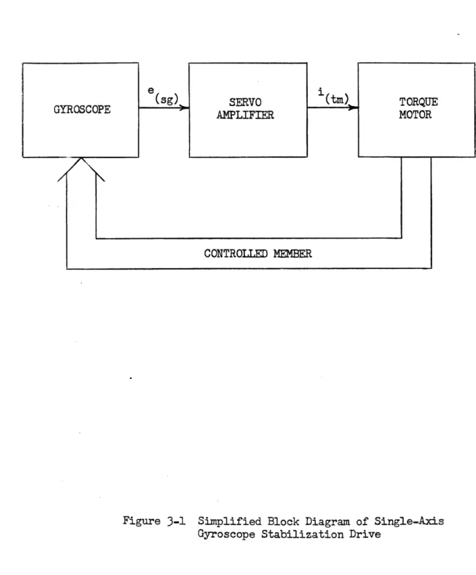
Figure
+7
Documents relatifs