HAL Id: hal-01259829
https://hal.archives-ouvertes.fr/hal-01259829
Submitted on 26 May 2016
HAL is a multi-disciplinary open access
archive for the deposit and dissemination of
sci-entific research documents, whether they are
pub-lished or not. The documents may come from
teaching and research institutions in France or
abroad, or from public or private research centers.
L’archive ouverte pluridisciplinaire HAL, est
destinée au dépôt et à la diffusion de documents
scientifiques de niveau recherche, publiés ou non,
émanant des établissements d’enseignement et de
recherche français ou étrangers, des laboratoires
publics ou privés.
structure due to aerosol variations
Steven T. Massie, Julien Delanoë, Charles G. Bardeen, Jonathan H. Jiang, Lei
Huang
To cite this version:
Steven T. Massie, Julien Delanoë, Charles G. Bardeen, Jonathan H. Jiang, Lei Huang. Changes in the
shape of cloud ice water content vertical structure due to aerosol variations . Atmospheric Chemistry
and Physics, European Geosciences Union, 2016, 16 (10), pp.6091-6105. �10.5194/acp-16-6091-2016�.
�hal-01259829�
www.atmos-chem-phys.net/16/6091/2016/ doi:10.5194/acp-16-6091-2016
© Author(s) 2016. CC Attribution 3.0 License.
Changes in the shape of cloud ice water content vertical structure
due to aerosol variations
Steven T. Massie1,3, Julien Delanoë2, Charles G. Bardeen3, Jonathan H. Jiang4, and Lei Huang4
1Laboratory for Atmospheric and Space Physics, University of Colorado, Boulder, Colorado, USA 2LATMOS/IPSL/UVSQ/CNRS, Guyancourt, France
3National Center for Atmospheric Research, Atmospheric Chemistry and
Modeling, Boulder, Colorado, USA
4Jet Propulsion Laboratory, California Institute of Technology, Pasadena, California, USA Correspondence to: Steven T. Massie ([email protected])
Received: 17 September 2015 – Published in Atmos. Chem. Phys. Discuss.: 21 January 2016 Revised: 22 April 2016 – Accepted: 1 May 2016 – Published: 19 May 2016
Abstract. Changes in the shape of cloud ice water
con-tent (IWC) vertical structure due to variations in Moderate Resolution Imaging Spectroradiometer (MODIS) aerosol op-tical depths (AODs), Ozone Monitoring Instrument (OMI) absorptive aerosol optical depths (AAODs), and Microwave Limb Sounder (MLS) CO (an absorptive aerosol proxy) at 215 hPa are calculated in the Tropics during 2007–2010 based upon an analysis of DARDAR IWC profiles for deep convective clouds. DARDAR profiles are a joint retrieval of CloudSat-CALIPSO data. Analysis is performed for 12 sep-arate regions over land and ocean, and carried out applying MODIS AOD fields that attempt to correct for 3-D cloud ad-jacency effects. The 3-D cloud adad-jacency effects have a small impact upon our particular calculations of aerosol–cloud in-direct effects. IWC profiles are averaged for three AOD bins individually for the 12 regions. The IWC average profiles are also normalized to unity at 5 km altitude in order to study changes in the shape of the average IWC profiles as AOD in-creases. Derivatives of the IWC average profiles, and deriva-tives of the IWC shape profiles, in percent change per 0.1 change in MODIS AOD units, are calculated separately for each region. Means of altitude-specific probability distribu-tion funcdistribu-tions, which include both ocean and land IWC shape regional derivatives, are modest, near 5 %, and positive to the 2σ level between 11 and 15 km altitude. Similar analy-ses are carried out for three AAOD and three CO bins. On average, the vertical profiles of the means of the derivatives based upon the profile shapes over land and ocean are smaller for the profiles binned according to AAOD and CO values,
than for the MODIS AODs, which include both scattering and absorptive aerosol. This difference in character supports the assertion that absorptive aerosol can inhibit cloud devel-opment.
1 Introduction
Uncertainty in aerosol effects upon clouds remains the largest of the global climate forcing uncertainties (Stocker et al., 2013). Tao et al. (2012) discuss the various types of aerosol indirect effects (e.g., effects on cloud droplets and ice particles, reflectance, cloud heights, lifetime, coverage, and precipitation). Though various aerosol indirect effects have been identified, there remains much quantitative uncertainty. By the cloud invigoration mechanism (Rosenfeld et al., 2008), an increase in aerosol is expected to modify the man-ner in which vertical and horizontal cloud structure devel-ops in deep convective clouds. The cloud invigoration mech-anism is of fundamental importance in regard to aerosol in-direct effects upon deep convective clouds. It is expected that the vertical ice water content (IWC), particle radii, and heat-ing rate profiles of a deep convective cloud differ under low and high aerosol optical depths (AODs) due to different ini-tial cloud condensation nuclei (CCN) values in the lower por-tion of the cloud. A change in the CCN concentrapor-tion alters the formation rate and size of liquid droplets, allowing more water to be transported above the freezing level, which leads to a perturbed vertical profile of latent heat release, and
sub-sequent invigoration of cloud development. This invigoration effect will occur throughout the cloud, changing IWC verti-cal structure.
The literature of observed and modeled aerosol indirect effects, however, is characterized by a variety of conclusions with differences in even the sign of the effects. For exam-ple, Koren et al. (2010) analyzed moderate resolution imag-ing spectroradiometer (MODIS) AOD and cloud top pressure data for July–August 2007 over the Atlantic west of equa-torial Africa for low and high clouds. For high clouds near 370 hPa (i.e., 7 km altitude, see Fig. 6 of Koren et al., 2010), cloud top pressure changed by −7 % / 0.1 AOD (i.e., cloud top heights increased as AOD increased). In this paper we use % change per 0.1 AOD units in order to compare the cal-culations from several studies. Assuming that the cloud top position is dependent upon the location of cloud vertical op-tical depths near unity, a decrease in cloud top pressure cor-responds to moving the optical depth profile upwards in alti-tude. IWC is then +7 % / 0.1 AOD larger at the position of the higher cloud top. In contrast, Wall et al. (2014) studied con-gestus (4–8 km altitude range), analyzing 14 years of Trop-ical Rainfall Measuring Mission (TRMM) radar precipita-tion features, and 6 years of CloudSat radar reflectivity data. Aerosol Index (AI) data (i.e., AI is the product of MODIS AOD and the MODIS Ångström exponent) were collocated with the TRMM and CloudSat data. TRMM echo-top heights increased with increasing AI over the Amazon and Africa, and decreased over the equatorial Atlantic and southwest United States. Differences in CloudSat maximum reflectivity means of clean and dirty congestus were statistically signif-icant at the 99 % level below 4 km over the Amazon, and at 4–5 km over Africa, but not at higher altitudes.
It is important to note that changes in particle radius due to changes in aerosol also result in IWC profile perturbations, even in the absence of convective invigoration. Morrison and Grabowski (2011) used a two-dimensional cloud-system re-solving model to investigate aerosol indirect effects for pris-tine, polluted, and highly polluted conditions during a 6-day period of active monsoon conditions. The ensemble calcu-lations indicated a small weakening of convection, higher cloud top heights and anvil ice mixing ratios for the polluted cases. Smaller ice particle sizes and smaller fall velocities perturbed the IWC profiles. Fan et al. (2013) used the NCAR WRF model, coupled to a spectral-bin microphysics code, to simulate deep convective clouds (DCC) for 1 month for three different regions over the tropical western Pacific (i.e., the TWP-International Cloud Experiment), southern China, and over the US southern Great Plains ARM site. They found “that although the widely accepted theory of DCC invigo-ration due to aerosol’s thermodynamic effect (additional la-tent heat release from freezing of greater amount of cloud water) may work during the growing stage, it is the micro-physical effect influenced by aerosols that drives the dra-matic increase in cloud cover, cloud top height, and cloud thickness at the mature and dissipation stages by inducing
larger amounts of smaller but longer-lasting ice particles in the stratiform/anvils of DCCs, even when thermodynamic in-vigoration is absent”.
Increases in AOD will invigorate for small AODs, though inhibit convection at larger AODs, since larger AODs de-crease the amount of sunlight which reaches the surface. Based upon application of a pseudo-adiabatic parcel model, Rosenfeld et al. (2008) estimated that maximum release of convective energy occurs for AODs near 0.3. The contrast-ing influences of cloud microphysics and radiative processes, and their influence on cloud fraction were parameterized in analytic equations by Koren et al. (2008), and validated by an analysis of MODIS AODs, cloud fractions, and cloud top pressure observed over the Amazon in the dry season. The upper panel of Fig. 2 of Koren et al. (2008) indicates that cloud top pressures are lowest (i.e., cloud top heights are highest) for AODs near 0.4.
It is also possible that absorptive AOD can inhibit cloud development. Ramanathan et al. (2005) used model simula-tions to study the influence of absorptive aerosol offshore of India. The model aerosol perturbed temperature profile ver-tical gradients in the first several kilometers near the surface, yielding a stabilizing influence upon cloud development. Ra-manathan et al. (2007) deployed small aerial aircraft over the Maldives in 2006 to measure aerosol characteristics during time periods with and without enhanced aerosol amounts. Heating rate calculations indicated that the enhanced aerosol produced a vertical temperature profile that was more stable, and therefore likely inhibited cloud development.
According to the theory, buoyancy increases by the re-lease of latent heat, and decreases when condensate load-ing (i.e., the weight of liquid or ice in a fluid parcel) in-creases (see Eqs. (2.50)–(2.53) of Houze, 2014). Lebo and Seinfeld (2011) state that “the aerosol-induced effect is con-trolled by the balance between latent heating and the increase in condensed water aloft, each having opposing effects on buoyancy.” Since changes in buoyancy can be positive or negative, depending upon specific situations in which latent heating or condensate perturbations are dominant, changes in cloud structure IWC likely could be positive or negative as AOD increases.
Lebo and Seinfeld (2011) modeled aerosol effects on deep convection by applying the Weather Research and Forecast-ing (WRF) model as a cloud resolvForecast-ing model, with separate bulk and bin microphysics schemes. Figure 6 of Lebo and Seinfeld (2011) presents domain averaged liquid and IWC profiles at 2, 4, and 6 h for “Clean”, “Semi-Polluted”, and “Polluted” scenarios, with cloud condensation nuclei (CCN) values of 100, 200, and 500 cm−3, respectively. The three IWC profiles for the three CCN values are equal to each other at 5 (6) km altitude for the bulk (bin) microphysics schemes, respectively, and then diverge at higher altitudes. This diverg-ing characteristic indicates that the shape of the IWC profile changes as AOD changes. This Figure motivates us to calcu-late IWC average profiles for individual regions in the
Trop-ics, and IWC shape profiles, for several AOD bins. The IWC shape profiles are obtained by normalizing the IWC average profiles to unity at 5 km altitude.
There are noticeable differences in the bulk and bin mi-crophysics model calculations in Fig. 6 of Lebo and Sein-feld (2011). The bulk scheme IWC profiles differ by −5 % at the IWC peak near 6 km altitude, indicating a decrease in IWC as aerosol increases, while the bin microphysics IWC profiles differ by 120 % at the IWC peak near 9 km alti-tude, indicating a large increase in IWC as aerosol increases. Figure 1 of Rosenfeld et al. (2008), which graphs 500 nm AOD as a function of CCN, can be used to estimate AODs that correspond to the model CCN values. The difference in AOD between the Clean and Polluted CCN values is approx-imately 0.094. The 120 % increase in IWC therefore trans-lates to an increase in IWC of 127 % per 0.1 AOD. Lebo and Seinfeld (2011) attribute the bulk and bin microphysics model differences to differences in vertical motion and parti-cle size (sedimentation) characteristics of the two microphys-ical schemes.
Storer and van den Heever (2013) modeled deep convec-tive clouds by running the Regional Atmospheric Modeling System (RAMS) (Cotton et al., 2003) in a 2-D radiative-convective equilibrium framework. Six CCN loadings be-tween 100 and 3200 cm−3 were applied in separate calcu-lations. After a 60-day initialization, model output was sam-pled every 5 min during a 10-day period. They note that early storm updrafts were influenced by increased latent heating, while more mature updrafts were largely influenced by in-creased drag from condensate loading. Differences in buoy-ancy curves for “polluted” and “clean” aerosol cases (see Fig. 8 of Storer and van den Heever, 2013) indicate that la-tent heating effects were numerically smaller, by an order of magnitude, than those due to condensate loading. The num-ber of cloud-top counts, averaged over 10 days, shifted to-ward higher and medium cloud tops and fewer low cloud tops (see Fig. 1 of Storer and van den Heever, 2013). The freezing level was near 4.4 km, with low, medium, and high cloud tops defined for altitudes less than 4.4, 4.4–10 km, and altitudes greater than 10 km, respectively. On a percentage basis, medium and high cloud top heights increased by ap-proximately 3 and 5 %, respectively, between the 100 and 400 cm−3 CCN values. The 100 and 400 cm−3 CCN val-ues are closest in value to those used in the Lebo and Se-infeld (2011) calculations discussed above.
Changes in the shape of cloud ice water content verti-cal structure, and changes in IWC vertiverti-cal profiles, due to aerosol variations in moderate resolution imaging spectro-radiometer (MODIS) aerosol optical depths (AODs), Ozone Monitoring Instrument (OMI) absorptive aerosol optical depths (AAODs), and Microwave Limb Sounder (MLS) CO (an absorptive aerosol proxy) at 215 hPa, are calculated in this paper for the Tropics over land and ocean during 2007– 2010 based upon an analysis of DARDAR IWC profiles of deep convective clouds. DARDAR profiles (Delanoë and
Hogan, 2008, 2010) are a joint radar-lidar retrieval using CloudSat radar reflectivity and CALIOP lidar observations at 532 nm. We carry out our calculations over several years (2007–2010), individual regions and seasons, in order to build up statistics. Section 2 discusses the data used in our study, Sect. 3 discusses the Methodology which is applied in a similar manner to the AOD, AAOD and CO data, and re-sults are presented in Sect. 4. A discussion of the rere-sults and conclusions are presented in Sect. 5.
2 Data
Ice water content vertical profiles are from the v2.1.0 DARDAR (raDAR/liDAR) data archive (http://www.icare. univ-lille1.fr/drupal/archive/) of the ICARE Thematic Cen-ter. The DARDAR cloud product is derived using the Varcloud algorithm (Delanoë and Hogan, 2008) and uti-lizes CloudSat reflectivity, and CALIOP lidar backscatter at 532 nm to jointly retrieve the properties of ice clouds (e.g., IWC, visible extinction, effective cloud particle ra-dius). There is one DARDAR profile, with a vertical reso-lution of 60 m, for every CloudSat radar profile and there-fore an along-track horizontal resolution of 1.7 km. Cloud-sat (Stephens et al., 2002) and the CALIOP lidar (on the CALIPSO satellite, Winker et al., 2010) were launched in tandem in 2006 as part of the A-Train. We analyze data from all months of 2007 through 2010.
The DARDAR retrieval algorithm is discussed in Delanoë and Hogan (2008, 2010). The applied optimal estimation technique (see Rodgers (2000) for a general discussion) in-corporates up to date aircraft particle size distribution and habit information to formulate forward model look-up ta-bles. The lidar forward model uses a fast radiative transfer code (Hogan, 2006). The combination of 95 GHz CloudSat radar and 532 nm CALIOP lidar observations provide infor-mation on both small and larger ice particles, since Cloud-Sat and CALIOP are sensitive to larger and smaller particles, respectively. Since the lidar is subject to strong attenuation, the radar measurement takes over for thick ice clouds. The radar-lidar overlap region allows one to retrieve simultane-ously size and concentration information. For this reason the combination of the two measurements improves the retrieval of cloud properties compared to single instrument retrievals. The DARDAR data focus on ice particles, so our analysis is restricted to altitudes above 5 km.
Deng et al. (2013) found reasonable agreement between CloudSat-CALIPSO (2C-ICE) and DARDAR retrieval prod-ucts. IWC values from 2B-CWC-RO, 2C-ICE, and DAR-DAR generally are in good agreement, while 2B-CWC-RVOD radii were 40 % larger than the 2C-ICE and DARDAR radii.
One stated concern in aerosol-indirect effect studies is that it is difficult to measure aerosol optical depths near clouds using nadir view satellite instruments. A cloud away from an observation point scatters light from the cloud towards the nadir observation point, which is then scattered towards the satellite sensor. Varnai and Marshak (2009) quantified how MODIS reflectance is enhanced as a function of dis-tance to the nearest cloud. The reflecdis-tance is enhanced by
∼10 % when clouds are 5 km away from clear sky footprints at a wavelength of 0.68 µm. Zhang et al. (2005) compared AERONET and MODIS MOD04 AODs. They demonstrate that MODIS AODs are enhanced at cloud edges, with dif-ferences between MODIS and AERONET AODs increasing as the cloud fraction increases, while the AERONET values stay relatively constant. We address this concern in our cal-culations by using the latest V6 MODIS aerosol data that in-clude a parameter indicating the average pixel distance from a measured AOD to the nearest cloud feature.
MODIS version 6 MYD04 data files are used to spec-ify daily aerosol optical depth fields. In particular, we uti-lize the “Optical_Depth_Land_and_Ocean” AOD values at 0.55 µm, which are specified at 10 km horizontal spatial res-olution. We process the 10 km AODs into daily data files at 1◦×1◦longitude–latitude resolution for 25◦S to 25◦N. As discussed by Levy et al. (2013), the Collection 6 (hence-forth C6) aerosol retrieval algorithms have made several improvements compared to the C5 data. The C6 “Aver-age_Cloud_Pixel_Distance_Land_Ocean” variable specifies the number of pixel units from an AOD to the nearest cloud pixel. Pixel unit distances are on the order of 0.5 km. We use this variable to calculate separate 1◦×1◦AOD fields for
several “cloud screening” cases. For the first case, all AODs are used within a 1◦×1◦ grid box if the AOD is between
10−3 and 3. Another set uses all AODs that are, e.g., 2 or more pixel units from MODIS clouds. Daily 1◦×1◦ fields of AODs for 2, 4, and 6 pixel units, and the “all AOD” case, are calculated separately for 25◦S to 25◦N. As discussed in the next section, the AOD fields are used in separate calcula-tions, for each pixel-distance case, to assess the sensitivity of the calculations to 3-D cloud adjacency effects. The AODs used in our processing are for quality flag 3 (i.e., only the best quality data are used).
Levy et al. (2014) discuss the differences in C6 and C5 Aqua MODIS AODs. C6 AODs increase by 0.05 over the tropical ocean and the Amazon, decrease by −0.05 over the southern oceans and northern mid-latitudes, and increase by 0.02 on a global basis. C6 AODs over land increased by 0.10 over East Asia, vegetation, Africa, Eastern United States, and decreased over the Western United States, South Africa, and semi-arid regions. The correlations of MODIS and AERONET AODs change slightly from 0.928 to 0.937 for the C5 and C6 data, respectively. Expected errors for C6 AODs over the ocean are −0.02 (−10 %) and +0.04 (+10 %) and over Land by ±(0.05 + 15 %).
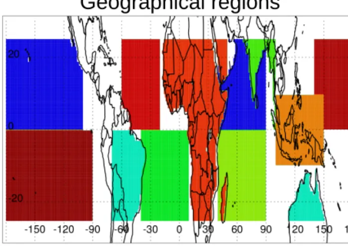
Geographical regions
Figure 1. Geographical Tropical regions over land and ocean.
The OMI OMAEROe data are contained in grid-ded (level 3) hdf files with a resolution of 1/4◦×1/4◦ (http://disc.sci.gsfc.nasa.gov/Aura/data-holdings/OMI/ omaeroe_v003.shtml). These data files utilize for each grid cell the level 2 data that has the shortest sun to sensor path length. The data are derived from a multi-wavelength aerosol retrieval algorithm (Veihelmann et al., 2007; Veihelmann and Veeefkind, 2009) that uses 14 bands and a look up reflectance table, calculated for four aerosol model types (desert dust, biomass burning, volcanic, and weakly absorb-ing aerosol), size distributions, and aerosol layer altitudes. The level 2 data are calculated by minimizing the differences between observed and model reflectance values.
MLS CO (http://disc.sci.gsfc.nasa.gov/Aura) at 215 hPa is an aerosol proxy (Jiang et al., 2008, 2009). CO is a byprod-uct of incomplete combustion of biofuels and fossil fuel, and is associated with soot (which absorbs light). CO is retrieved from microwave radiances in two bands of the 240 GHz radiometer (Livesey et al., 2008). Level 2 version 4.2 profiles have a vertical resolution of 3.5–5 km in the upper troposphere. We grid CO measurements at 215 hPa into daily 1◦×1◦ data files. As discussed in Livesey et al. (2015), 215 hPa is the highest pressure (lowest altitude) for which data applications are recommended. The 215 hPa data have a precision of 19 ppbv and a systematic uncertainty of ±30 ppbv (±30 %).
3 Methodology
Figure 1 presents the various regions in the Tropics for which we calculate average IWC profiles. The 12 regions are either over land or ocean since cloud dynamics differ over land and ocean (Houze, 2014), cloud dynamics likely vary from re-gion to rere-gion due to various topographical and surface heat-ing characteristics, and cloud activity peaks at different local times on a regional basis (Liu and Zipser, 2008). We focus on the Tropics in this study to avoid mid-latitude complications
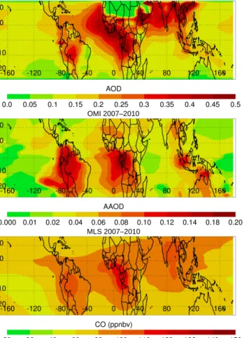
MODIS 2007–2010
OMI 2007–2010
MLS 2007–2010
Figure 2. Average MODIS AOD, OMI AAOD, and MLS CO at 215 hPa for 2007–2010.
due to frontal dynamics. The 12 regions cover most of the Tropics, are limited in longitude, and include as many IWC profiles as possible in order to reinforce the statistics.
The general distribution of MODIS AOD, OMI AAOD, and MLS CO, averaged over all seasons between 2007 and 2010, is presented in Fig. 2. The largest AODs originate from land regions over Africa, South America, Southeast Asia, and Indonesia. There are few 0.55 µm AODs over North Africa. This is due to the large surface albedo of desert sands, for which it is difficult for MODIS to detect suspended aerosols. AODs, AAODs, and CO values are generally larger over land than ocean. Large AODs, AOODs, and CO are observed off-shore of Africa due to transport of mainland aerosol to the adjacent ocean areas. Absorptive aerosol is prevalent over South America and Africa due to the prevalence of biomass burning in these regions.
An example of the IWC structure of a deep convective cloud, observed near 111◦W and 8◦N on July 10, 2007, is presented in Fig. 3. DARDAR IWC, with original units of kg m−3is rescaled for graph clarity purposes. Two hun-dred and forty individual profiles were measured in this deep convective cloud. In general, IWC increases in value from the top of the cloud downwards, reaches a maximum value,
IWC (kg m )-3
Figure 3. DARDAR IWC structure of a tropical cloudy region ob-served on 10 July 2007.
Step 1 Step 2 Step 3 Step 4 Step 5
IWCreg IWCreg,derivatives IWCreg,derivative pdfs
IWCdaily IWCsum
IWCshape IWCshape,derivatives IWCshape,derivative pdfs
Figure 4. Summary of the processing steps.
then decreases somewhat. For this cloudy region, latitude and height variations in IWC are apparent, since the heights of the top of the cloud and the maximum IWC values vary as a function of latitude.
Based upon the original DARDAR data files, we proceed in several steps, processing both day and night profiles. We first process the DARDAR data into daily files of IWC pro-files (i.e., IWC daily). An original profile is retained if the profile has IWC greater than 5 × 10⁻⁵kg m−3and less than 0.05 kg m−3 (i.e., near the high end of the retrieval) and if the IWC values are contiguous for two or more kilometers in vertical extent. This Step 1 processing is helpful due to the large data volume (i.e., 1.9 TB, 8.2 × 10⁶profiles for the
Tropics) of the original DARDAR data files. This Step and subsequent processing steps are summarized in Fig. 4.
The Step 2 processing of the DARDAR and AOD data produces yearly files of deep convective cloud structure for 2007–2010. Step 1 profiles are used if the vertical depth of the profile is at least 5 km above 5 km altitude. Step 1 IWC profiles are collocated with the daily MODIS AOD files to calculate IWCsum profile sums, binned according to AOD, longitude, latitude, aerosol to cloud pixel distance, season, and altitude.
IWCsum (AOD, longitude, latitude, pixel distance, season, altitude)
=6IWCdaily (1)
There are three MODIS AOD bins, 72 longitude and 11 lat-itude bins at 5◦ resolution, four cloud-screening cases (for “all AOD”, 2, 4, and 6 pixel-distance cases), four seasons, and 131 altitude steps in 0.1 km increments from 5 to 18 km altitude. IWCsum units are in kg m−3. The three AOD bins
stated in Table 1 (i.e., 0.01–0.15, 0.15–0.30, 0.30–0.45) were chosen to represent low, medium, and high amounts of AODs (as indicated by inspection of MODIS AOD probability dis-tribution functions, PDFs). The MODIS AOD PDFs (not shown) indicate that there are relatively few MODIS AODs greater than 0.45. AAOD and CO bins are also specified in Table 1. The bin ranges were selected from examination of, e.g., x = MODIS AOD vs. y = OMI AAOD scatter dia-grams, which indicated the range of OMI AAOD correspond-ing to each MODIS AOD bin range. The AOD vs. AAOD and AOD vs. CO scatter diagrams places the AOD, AAOD, and CO calculations on an approximate equal footing.
Step 3 of the processing sorts the IWCsum data into IWCreg regional averages, binned according to AOD, region, aerosol to cloud pixel distance, season, and altitude.
IWCreg (AOD, region, pixel distance, season, altitude)
=6IWCsum (AOD, longitude, latitude, pixel distance, season, altitude) (2) This calculation averages data into seven altitude bins of 2 km vertical extending from 5 to 18 km altitude. IWCreg units are in kg m−3. The reason for the vertical binning is to promote as much statistical significance as possible from the averaging process. The number of IWC profiles in a single re-gion and altitude bin varies from less than 103to greater than 9 × 10⁴ since AODs are generally smaller over the oceans and the regions vary in spatial extent.
We also calculate normalized IWC profiles (i.e., IWC-shape profiles) based upon the IWCreg profiles by dividing the IWCreg profile by the IWCreg value in the 5 to 7 km bin range.
IWCshape (AOD, region, pixel distance, season, altitude)
=IWCreg (AOD, region, pixel distance, season, altitude)/ IWCreg (AOD, region, pixel distance, season,
altitude from 5 to 7 km) (3)
The IWCshape array, in dimensionless units, has the same binning as the IWCreg array. The IWCshape profile is of course 1.0 for the 5–7 km bin, and deviates from unity at higher altitudes, indicating how the shape of the IWC struc-ture progressively changes above 7 km altitude. As noted above, the calculation of the IWCshape profiles is moti-vated by the profiles displayed in Fig. 6 of Lebo and Sein-feld (2011) since modeled IWC profiles for the three model CCN values diverge at altitudes greater than 5 km altitude.
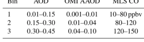
Table 1. AOD, AAOD, and 215 hPa CO bins used in this study.
Bin AOD OMI AAOD MLS CO
1 0.01–0.15 0.001–0.01 10–80 ppbv 2 0.15–0.30 0.01–0.04 80–120 3 0.30–0.45 0.04–0.10 120–150
Another reason to look at the shape of IWC structure is that observational sampling of a cloudy region for the three AOD bins is not a precisely “controlled” process. A cloudy region has a 3-D IWC structure with 3-D variations in IWC. The CloudSat and CALIPSO sampling of 3-D IWC struc-tures (i.e., a vertical 2-D slice through the cloudy region, with a corresponding set of 1◦×1◦ MODIS AODs) is random.
One random sampling of a cloudy region could be weighted by more observations with lower IWC values, and another random sampling could be weighted by higher IWC values. If the sampling of 3-D cloudy regions, with respect to low and high regions of IWC, is not consistently similar for the three bins of AOD, then a sampling issue arises. By looking at the shape of the vertical IWC structure one can attempt to mitigate this sampling issue, by putting the IWCreg average profiles for the three AOD bins on a normalized footing. It is reasonable to assume that this sampling issue becomes less of a concern when the number of profiles for a given region and season increases.
In Step 4 of the processing, derivatives are calculated two ways. ∂IWCreg/∂AOD derivatives (henceforth, IWCreg derivatives) are first calculated for each region, season, and pixel-distance AOD field at each of the seven altitude bins. The value of the IWCreg derivative is the average of two derivatives, based upon IWCreg values at the first and sec-ond, and first and third, aerosol bins.
∂IWCreg/∂AOD (region, season, pixel distance, altitude)
=0.5 {(IWCreg (2, . . .) − IWCreg (1, . . .))/
(AOD(2) − AOD(1)) + (IWCreg (3, . . .)
−IWCreg (1, . . .)) /(AOD(3) − AOD(1))} , (4)
where numbers (e.g., 2) refer to the AOD bin of Table 1, and . . . refers to the region, season, pixel distance, and altitude bins. This average derivative is then transformed, for graphical and other purposes, into percent change per 0.1 AOD units by dividing the derivative by the average IWCreg value. ∂IWCshape/∂AOD derivatives (henceforth, IWCshape derivatives) are then calculated for the seven al-titude bins in similar fashion.
Equations (1)–(4) are applied to the IWC profiles using OMI AAOD and MLS CO values, separately, in place of the MODIS AOD data. The transformed AAOD and CO deriva-tives are in % per 0.02 AAOD and % per 100 ppbv units, respectively. The AAOD and CO derivatives are binned
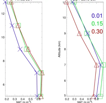
ac-IWC (g m )-3 IWC (g m )-3 Figure 5. Average IWCreg vertical profiles over SE Pacific during December–January–February and over Africa during June–July– August for MODIS aerosol bins with lower bin limits of 0.01, 0.15, and 0.30. Data have been averaged into 2 km bins of vertical alti-tude.
cording to region, season, pixel distance, and altitude, in the same way as for the AOD derivatives.
In Step 5 of the processing, we place the IWCreg deriva-tives for the various regions and seasons into PDFs at each of the seven altitude bins. PDFs are constructed separately from the AOD, AAOD, and CO derivatives. Derivatives are included in the PDF if the number of IWC profiles in a derivative is greater than 103. (The 103threshold was empir-ically determined based upon visual examination of individ-ual IWCreg profiles). We calculate the means of the PDFs, standard deviations from the means, and 95 % (2σ ) confi-dence levels of the means of the PDFs. In a similar manner, the IWCshape derivatives are used to calculate the means of PDFs and 95 % confidence limits of the means of the PDFs. As discussed below, we examine and compare the means of the various PDFs.
Finally, an additional separate processing goes back to Step 2 and assigns MODIS AODs at a given 1◦×1◦grid box to the AOD at that position using a randomly chosen day dur-ing the year of interest. Ideally, random AODs should yield means of the PDF of the derivatives that are close to zero, since the ∂IWCreg/∂AOD and ∂IWCshape/∂AOD deriva-tives are reversed in sign if low and high values of AOD are interchanged. We compare the PDF means of this separate processing with those of the previous paragraph.
4 Results
Figure 5 illustrates the average vertical structure of IWCreg over Africa during summer (June–July–August) and over the southeast Pacific during winter (December–January– February). The mark at 5 km specifies the average between 5 and 7 km altitude, etc. The IWCreg values over Africa in-crease as AOD inin-creases for nearly every altitude level. In contrast, the IWCreg curves over the southeast Pacific in-crease from the first to second bin for the 5 to 9 km range, while decreasing for the first and third aerosol bins. These curves illustrate that derivatives for specific regions and sea-sons can be either positive or negative.
These curves also indicate that calculations of derivatives need to be confined to specific regions. There are height dif-ferences at which a specific IWC value is observed, e.g., 0.3 g m−3occurs at 11 km over the SE Pacific and at 10.5 km
over Africa for the 0.01–0.15 AOD bin. Global calculations which lump together profiles from different regions mix IWC profiles of different height characteristics, due to regional differences in, e.g., cloud type and/or weather conditions. If the number of regional profiles varies from region to re-gion for a specific AOD bin, and these profiles have differ-ent average height characteristics, then the derivatives calcu-lated using the globally lumped profiles are prone to error (since differences in the average regional profiles are related to both AOD effects and regional differences due to cloud type and/or weather conditions).
The impact of cloud adjacency effects upon the AOD fields is illustrated in Fig. 6. Daily MODIS C6 AOD data fields were averaged for 25◦S to 25◦N for “all AOD”, 2, 4, and
6 pixel-distance cases. On the x axis the AODs correspond to the case when all AODs in the 1◦×1◦grid box are used
to define the AOD field. On the y axis is the ratio of the AODs for a particular pixel-distance to the “all AOD” case. The ratios for all of the curves are smallest for the smaller AODs, and increase to larger values as the AODs increase. The AODs are approximately 2 % smaller for the 2 pixel-distance case compared to the “all AOD” case. As more and more AODs are tossed out of the screening process, the AOD averages become progressively smaller than the “all AOD” case, up to 8 % for the 6 pixel-distance case. Unfortunately, the number of nonzero 1◦×1◦grid box AODs decreases for the 4 and 6 pixel-distance cases. Use of the 2 pixel-distance field is more practical than the other cases. Since each AOD bin range in our Step 2 binning processing covers a large range in AOD, a 2 % effect likely places an “all AOD” and, e.g., “2 cloud pixel distance” AOD into the same AOD bin range. It is therefore expected that correction for the cloud adjacency effect, using the three AOD bin ranges mentioned above in Sect. 3, will be of second order in our particular calculations.
–
Figure 6. Curves of 1◦×1◦MODIS V6 AOD averages, calculated with and without cloud pixel-distance screening. x axis AOD values are calculated using all MODIS AOD data, and y axis AODs are calculated by averaging AODs such that the AODs in the 1◦4× 1◦ geographical area are at 2, 4, and 6 pixel-distances from clouds. Data from 2007–2010, for 25◦S–25◦N, are used.
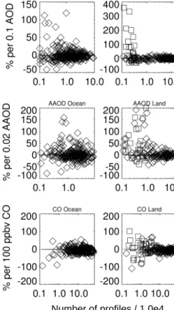
In Fig. 7 the statistical distribution of AOD, AAOD, and CO IWCreg derivatives for individual regions and seasons are displayed separately over land and ocean. The x axis indicates the number of individual profiles associated with the derivative of a specific region and season, with IWCreg derivatives on the y axis. As explained in Sect. 3 (Step 4 processing), the value of the IWCreg derivative for a 2 km altitude bin is the average of two derivatives, based upon IWCreg values at the first and second, and first and third, aerosol bins. The absolute magnitude of the derivatives over land or ocean decreases as the number of profiles increases.
The largest derivatives in the AOD, AAOD, and CO panels are those over mainland India, which are assigned the square symbol in Fig. 7. The India land region has the smallest area of our 12 regions, yet is subject to complicated monsoon dy-namics, and with the presence of absorptive aerosols over the Tibetan Plateau, likely subject to the absorptive aerosol “elevated heat pump” mechanism (Lau et al., 2006). Absorp-tive aerosol above the Tibetan plateau is attributed to provide an elevated heating source which leads to enhanced circula-tion that will draw air from the surface upwards along the southern flank of the Himalayas. India likely is subject to some of the most complicated aerosol–cloud interactions in the world.
In calculations presented below, we present analyses in which the largest derivatives are included, and excluded, from the calculations. Derivatives are not used in the
exclu-Number of profiles / 1.0e4
Figure 7. Statistical distribution of IWCreg derivatives between 5 and 15 km altitude for individual regions and seasons as a function of the number of profiles used to define each derivative. Derivatives over mainland India are assigned a square symbol.
Table 2. Average IWCreg derivatives over ocean and land (in % / 0.1 AOD units) expressed as a function of average pixel-distance values used to derive the AOD fields. Numbers in parenthesis are the numbers of derivatives used to define each average IWCreg deriva-tive.
Altitude Ocean Land
(km) 0 2 4 pixels 0 2 4 pixels 13–15 4.4 5.1 −3.8 2.8 1.7 1.7 (47 42 27) (31 31 28) 11–13 0.6 −0.3 2.8 23.1 23.5 15.8 (53 53 46) (36 36 34) 9–11 −0.9 −0.2 −0.5 18.0 18.0 19.1 (54 54 48) (36 36 36) 7–9 −1.7 −0.2 0.5 6.5 6.8 6.6 (54 55 48) (36 36 36) 5–7 0.4 0.9 1.9 1.7 1.6 1.6 (54 54 48) (36 36 36)
sionary calculations if the number of profiles on average are less than 1000 and/or if the derivatives are greater than 100 % per 0.10 AOD, 100 % per 0.02 AAOD, or 100 % per 100 ppbv CO.
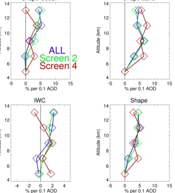
Figure 8. Curves of means of IWCreg and IWCshape PDFs illus-trating the sensitivity to the cloud-pixel distance AOD fields. “ALL” refers to the “All AOD” case, and corresponds to curves presented later in the text (i.e., Figs. 11 and 12).
Table 2 presents means of the PDFs for the IWCreg deriva-tives over land and ocean for the 2 km altitude bins, expressed as a function of the pixel-distance value. The means are culated assigning equal weight to each region (i.e., the cal-culations are not weighted by the number of profiles ob-served in each region). The number of statistically significant derivatives (i.e., number of separate regions and seasons) that went into the PDF decreases as the cloud pixel-distance value increases (since the number of AODs in the daily 1◦×1◦grid boxes decreases as the pixel-distance value increases). This is most apparent for the 4 pixel-distanced AOD fields. The PDF means in Table 2 are larger over land than the ocean, with fairly small modulation in these means due to pixel-distance choice.
Figure 8 illustrates how the means of curves presented later in the text (i.e., Figs. 11 and 12) are sensitive to the pixel-distance value. The means in Fig. 8 differ from those in Table 2 since the derivatives, used to calculate the curves in Figs. 11 and 12, are those less than 100 % per 0.1 AOD, while all derivatives are included in the Table 2 calculations. The “All AOD” case (i.e., “ALL in Fig. 8) and the Screen 2 (i.e., pixel-distance 2 AOD field) set of means are similar in Fig. 8.
Overall, it is apparent that the 3-D cloud adjacency effect has a fairly small impact upon the means of the PDFs in our calculations. For this reason, we henceforth focus on results
Figure 9. Vertical profiles of the means of the PDFs of IWCreg derivatives for individual regions and seasons based upon DAR-DAR IWC profiles, and MODIS AOD data for the “all AOD” case. Mean 95 % confidence (2σ ) limits are indicated by the horizontal lines. The symbol at 5 km denotes the average for the 5–7 km alti-tude range.
for the “all AOD” case in order to maximize the number of derivatives used in our calculations.
The means of the IWCreg derivative PDFs for the “all AOD” case are presented in Fig. 9 separately for land and ocean data. The 95 % confidence (2σ ) limits of the means are given by the horizontal lines. Over the ocean, the left panel of Fig. 9 indicates that the means are consistent with the zero % per 0.1 AOD line, as the zero % line falls between the 95 % confidence limits of the means. Over land the means are be-tween 10 and 20 % for the 9 to 13 km range, also consistent with the 0 % line.
Table 3 presents means of the PDFs for the IWCreg and IWCshape derivatives over land and ocean for the 2 km alti-tude bins, for the “all AOD” case. As before (see Table 2) the PDF IWCs derivative means over land are larger than those over the ocean, and the values increase with altitude. In ad-dition, the Rnd columns refer to calculations in which a dom day is calculated for each specific day, injecting a ran-dom AOD field into the calculations. If AODs are ranran-domly selected from the MODIS AODs, then the means of the PDFs of the IWCshape derivatives are small, though nonzero. We interpret the nonzero values near 2 % as evidence that the means of the cloud dynamic variables (e.g., surface humidity, CAPE, surface temperature, etc.) are different for the vari-ous AOD bins. The fact that the differences in the IWCshape and Rnd columns are positive (especially for the observa-tions over land) indicates that the cloud invigoration effect is nonzero and positive.
Table 3. Average IWCreg and IWCshape derivatives over ocean and land (expressed in % change in IWC/0.1 AOD units).
Altitude Ocean Land
(km) IWCreg Shape IWCreg Shape
IWCshape Rnd IWCshape Rnd 13–15 4.4 7.4 2.0 2.8 4.6 1.6 11–13 0.6 5.3 2.8 23.1 23.8 1.2 9–11 −0.9 5.4 2.2 18.0 14.5 0.1 7–9 −1.7 −0.2 1.2 6.5 3.0 −0.7 5–7 0.4 0.0 0.0 1.7 0.0 0.0
Rnd – same as IWCshape, with random MODIS AOD values used in the calculation.
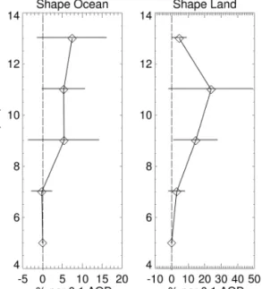
Figure 10. Vertical profiles of the means of the IWCshape regional and seasonal derivatives. MODIS “all AOD” data are used. Mean 95 % confidence (2σ ) limits are indicated by the horizontal lines.
Examination of individual derivatives over the ocean and land for the various altitude ranges indicates that most re-gions have positive and negative derivatives. This is consis-tent with our statements above in the Introduction that buoy-ancy is perturbed by both positive (latent heat) and nega-tive (condensate loading) influences. There are more posinega-tive ocean IWCreg derivatives north than south of the equator, with the largest annually averaged derivatives over the North-west and Northeast Pacific, and smallest derivatives over the South Atlantic. Largest annually averaged land derivatives are found over India, South America, and Africa, with small-est derivatives over Australia.
The means of the IWCshape derivative PDFs for the “all
AOD” case are presented in Fig. 10. Over the ocean and land the means are near 5 % and 10–20 % per 0.1 AOD for the 9 to 13 km range, respectively. The derivatives are positive to the 2σ level for the 9–11 and 13–15 km altitude ranges over
Figure 11. Same as Fig. 9 except that IWCshape derivatives less
than 100 % per 0.1 AOD are excluded from the averaging process.
land (i.e., the −95 % confidence limit of the mean value is positive for these two altitude ranges).
As remarked above, in regard to Fig. 7, the India aver-ages have a much smaller number of profiles than for other regions, since the geographical extent of this region is the smallest of the 12 regions. The IWCshape curves, from in-spection, are noisier than those of the other regions and the derivatives are substantially larger than those for the other regions. For this reason, it is appropriate to present calcula-tions in which India land derivatives, and those from other regions are excluded, if the number of profiles in an average is less than 1000 and the derivative is greater than 100 % per 0.10 AOD. Figure 11 presents calculations, similar to Fig. 9, except that the large derivatives are excluded from the calcu-lation. Over the ocean and land the means are near 5 and 4 % per 0.1 AOD, respectively, for the 9–13 km range.
Curves similar to Fig. 11 (not shown) were calculated for each Season of the year. Over land the Winter and Spring
Table 4. Percent of the observations indicating saturation and inhi-bition effects as MODIS AODs increase.
Altitude Saturation Inhibition
(km) Ocean Land Ocean Land
13–15 44 27 22 13
11–13 41 50 26 11
9–11 30 50 26 11
7–9 33 44 18 39
curves of the IWCshape means have altitude structure similar to Fig. 11 in that the means steadily increase as altitude in-creases. The Fall land means, however, are all near zero. Over the oceans the means are positive above 11 km altitude for all four seasons. The land and ocean seasonal means, however, are not statistically significant to the 2σ level.
As discussed in the Introduction, AODs are expected to invigorate convection for low AODs, with saturation appar-ent at larger AODs. These saturation effects start to occur for AODs near 0.30 and 0.40 as calculated by Rosenfeld et al. (2008) and Koren et al. (2008), respectively. These satu-ration onset AODs correspond to the third AOD range (0.35– 0.45) of our calculations. To quantify the percent of observa-tions which are consistent with this saturation scenario, we calculated for each region, season, and altitude, 1IWC(i, j ) differences
1IWC(i, j ) = IWCshape(i) − IWCshape(j ), (5)
where i or j refers to the aerosol bins 1, 2, 3 (i.e., the three MODIS aerosol bins in Table 1), respectively. If the first difference 1IWC(2, 1) was positive, and the differ-ence 1IWC(3, 2) was negative or less than the absolute value of the first difference, then this indicated saturation. With regards to inhibition, this scenario corresponds to the case in which the 1IWC(2, 1) and 1IWC(3, 2) values are both negative. Table 4 presents the percentages for which these two scenarios appeared in our calculations based upon the MODIS data. The saturation scenario occurred approxi-mately twice as often as the inhibition scenario. These per-centages are for “ideal” outcomes in which both 1IWC val-ues are used to identify one scenario or the other.
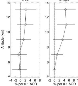
Figure 12 displays the means of PDFs specified by com-bining the land and ocean IWCshape derivatives, exclud-ing the largest derivatives, to obtain a Tropical average. The means of the shape derivatives are near 5 % per 0.1 AOD (as expected from Fig. 11), and positive to the 2σ level in the 11 to 15 km altitude range. Also displayed in Fig. 12 are means calculated using the IWCreg derivatives, again excluding the largest derivatives. The means are positive above 9 km al-titude, but not statistically significant at the 2σ level. The mean of the IWCreg derivatives in the 5–7 km altitude range is nonzero (i.e., 0.04) but very small.
Another way to look at the derivatives is by graphing PDFs of the derivatives. Figure 13 presents PDFs of the IWCshape
Figure 12. Means of PDFs of IWCreg and IWCshape derivatives over ocean and land, excluding derivatives greater than 100 % per 0.1 AOD. Mean 95 % confidence limits, given by the horizontal lines, indicate that IWCshape means are positive to the 2σ level for the 11–15 km altitude range.
derivatives for the AOD, AAOD, and CO data. Derivatives over the ocean and land regions (excluding the largest deriva-tives) were aggregated for the 7–13 altitude range. All PDFs have a main Gaussian-like distribution, with several smaller contributions outside of the primary distribution. Averages of the PDFs are indicated at the top of the panels. The arithmetic means of the PDFs are less for the AAOD and CO data than for the AOD data, with positive means for the AOD data, and negative means especially for the CO data. These results are supportive of the assertion that absorptive aerosol tends to inhibit cloud development.
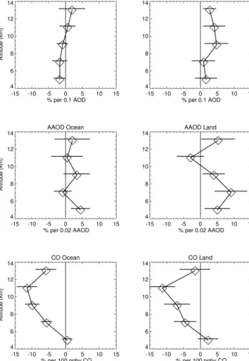
Figure 14 presents average IWCreg derivatives for AOD, AAOD, and CO data over ocean and land for all regions, excluding the largest derivatives. For legibility purposes, 1σ confidence limits of the determination of the means are given by the horizontal lines. The CO means over land and ocean are negative for the 7–15 km altitude range.
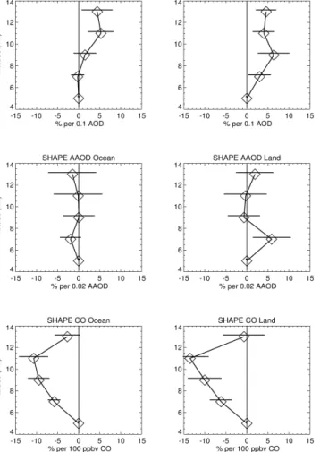
Finally, Fig. 15 is similar to Fig. 14 except that average shape derivatives are presented. The AAOD and CO shape derivative means are less than the AOD means both over ocean and land for the 9–15 km altitude range. These results are supportive of the assertion that absorptive aerosol tends to inhibit cloud development. It is notable in both Figs. 14 and 15 that the size of the mean derivatives are fairly small, with values mostly between −15 and 5 %.
Figure 13. Histograms of IWCshape derivatives for AOD, AAOD, and CO bins, when the derivatives are less than 100 % per 0.10 AOD, 100 % per 0.02 AAOD, and 100 % per 100 ppbv CO, respec-tively. Means of the distributions are indicated by the numbers in each panel’s title. Averages pertain to the 7–15 km altitude range.
5 Discussion
IWC increases slightly on average for deep convective clouds above the freezing level as AODs increase. The Tropical average means (Fig. 12), calculated using combined ocean and land IWCshape derivatives (excluding the largest deriva-tives) are near 5 % per 0.1 AOD above 9 km altitude, and positive to the 2σ level in the 11–15 km range. The 5 % per 0.1 AOD value is similar to the previously determined 7 % per 0.1 AOD value observed over the equatorial At-lantic region (corresponding to the cloud top pressure data of Fig. 6 from Koren et al., 2010), and similar to the 3–5 % increase in medium and high cloud tops calculated by Storer and van den Heever (2013), but substantially less than the
∼127 % / 0.1 AOD change in the IWC profile indicated by the bin microphysics calculations presented in Fig. 6 of Lebo and Seinfeld (2011).
As discussed above, the IWCreg average profiles are cal-culated without normalization at 5 km altitude. The IWCreg means in Fig. 12 are positive above 9 km but not statistically
Figure 14. Average IWCreg derivatives over ocean and land for AOD, AAOD, and CO. Derivatives were used when they were less than 100 % per 0.10 AOD, 100 % per 0.02 AAOD, and 100 % per 100 ppbv CO. Confidence limits (1σ ) of the determination of the means are indicated by the horizontal bars.
significant at the 2σ level. The lack of statistical significance is similar to the conclusions of Wall et al. (2014). One is struck by the fact that our study and that of Wall et al. (2014) both yield inconclusive aerosol indirect effects when many years of data are processed.
Figure 7 imparts an important lesson – the scatter in the measured derivatives decreases as the number of observed profiles in the various regions increases. We interpret Fig. 7 as follows. Changes in IWC vertical structure are due to both aerosol and cloud dynamic influences. For a specific region, a relatively small number of profiles will not likely sample the PDFs of all variables (aerosol and cloud dynamic variables such as surface and 500 hPa relative humidity, CAPE, wind shear, etc) as completely as for the case in which a larger number of profiles are considered. Differences in the average IWCreg profiles at different AODs can be due to differences in cloud dynamic differences, to a greater extent than to the AOD difference, depending upon circumstance, if the num-ber of observed profiles is relatively small. A negative (or
Figure 15. Average IWCshape derivatives over ocean and land for AOD, AAOD, and CO. Derivatives were used when they were less than 100 % per 0.10 AOD, 100 % per 0.02 AAOD, and 100 % per 100 ppbv CO. Confidence limits (1σ ) of the determination of the means are indicated by the horizontal bars.
large positive) derivative could be due to a change in cloud dynamic influences and not the AOD change. In addition, the CloudSat/CALIPSO observational 2-D “curtains” slice through a cloudy region. If the sampling of 3-D cloudy re-gions with respect to low and high rere-gions of IWC is not consistently similar for the, e.g., three bins of AOD, then a sampling issue arises. This sampling consideration becomes less of an issue when the number of observed profiles in-creases.
Interest in the cloud invigoration process is of course im-portant due to its consequences in regard to the radiative ef-fects of aerosol indirect efef-fects – perturbations in cloud ver-tical structure due to changes in aerosol translate into pertur-bations in the radiative effects of clouds upon climate. Un-derstanding the effects of aerosols upon cloud structure is a necessary step towards understanding the radiative effects. Global calculations which average regional and seasonal per-turbations of cloud structure over many years are of interest
since they yield a grand ensemble average that fully samples the PDFs of the aerosol and cloud dynamic variables.
It is apparent from our calculations that both invigoration processes (Rosenfeld et al., 2008; Koren et al., 2008) and inhibition processes (Ramanathan et al., 2005, 2007) are ex-pressed in our long-term derivatives which indicate that IWC can both increase or decrease as AOD increases. Changes in MODIS IWCshape profiles did indicate saturation effects as discussed by Koren et al. (2008). Saturation effects, in which an increase in IWC is followed by a small increase or de-crease in IWC, was present 32 % of the time (the average of the 1st and 2nd columns of Table 4). The means of the PDFs presented in Fig. 13, and the means of the IWCshape deriva-tives presented in Fig. 15 are also supportive of the assertion that absorptive aerosol can inhibit cloud development. Inhi-bition effects were present 17 % of the time (the average of 3rd and 4th columns of Table 4). The saturation scenario for MODIS data occurred approximately twice as often as the inhibition scenario.
Cloud adjacency (i.e., 3-D radiative transfer) issues are real, but the impact in our particular calculations is a second order effect. The 3-D cloud adjacency effects appear not to be a major impediment in regard to calculation of aerosol–cloud indirect effects, if the AOD bin ranges are fairly wide com-pared to the size of the 3-D effect (see Fig. 6). The variations in the IWCreg land derivatives in Table 2 for the “all AOD”, 2, and 4 pixel-unit cases is smaller than the altitude variations in the derivatives. We place an AOD into one of three AOD bin ranges. A 2 % AOD correction (see Fig. 6) due to cloud adjacency effects does not likely move the AOD from one bin range to another. As remarked above, the number of 1◦×1◦
AODs decrease as the pixel-distance unit increases. With the “all AOD” and 2 pixel-distance AODs giving similar deriva-tives over land in the right-hand portion of Table 2, and with the similarity in the curves presented in Fig. 8 for the three screening cases, the necessity to apply the pixel-distance cor-rection is debatable.
In conclusion, the literature of observed and modeled aerosol–cloud indirect effects is characterized by a range of results of different signed outcomes, including this study. This is due to the fact that numerous variables and many other physical considerations can influence whether a posi-tive or negaposi-tive effect is measured. In Fig. 15 there is a stark contrast between the positive AOD derivatives above 9 km altitude, and the negative CO derivatives. A portion of the contrasting positive and negative results reported in the lit-erature is likely due to whether or not absorptive aerosol is absent or present in a particular set of observations.
Data availability
DARDAR data were provided by CNES, and we thank the ICARE Data and Services Center (http://www.icare. univ-lille1.fr) for providing access to the data used in this study. OMI OMAEROe and MLS CO data were provided
by the NASA Goddard Earth Sciences Data and Infor-mation Services Center (http://disc.sci.gsfc.nasa.gov/Aura/ data-holdings/OMI/omaeroe_v003.shtml and http://disc.sci. gsfc.nasa.gov/Aura, respectively).
Acknowledgements. The work discussed in this paper is supported
by NASA Grants NNX14AL55G and NNX14AO85G. The Na-tional Center for Atmospheric Research (NCAR) is supported by the National Science Foundation. We also acknowledge the support by the Jet Propulsion Laboratory, California Institute of Technology, under contract with NASA.
Edited by: Q. Fu
References
Cotton, W., Pielke Sr., R. A., Walko, R. L., Liston, G. E., Tremback, C. J., Jiang, H., McAnelly, R. L., Harrington, J. Y., Nicholls, M. E., Carrio, G. G., and McFadden, J. P.: RAMS 2001: Current status and future directions, Meteorol. Atmos. Phys. 82, 5–29, 2003.
Delanoë, J. and Hogan, R. J.: A variational scheme for re-trieving ice cloud properties from combined radar, lidar, and infrared radiometer, J. Geophys. Res., 113, D07204, doi:10.1029/2007JD009000, 2008.
Delanoë, J. and Hogan, R. J.: Combined CloudSat-CALIPSO-MODIS retrievals of the properties of ice clouds, J. Geophys. Res., 115, D00H29, doi:10.1029/2009JD012346, 2010. Deng, M., Mace, G. G., Wang, Z., and Lawson, P. R.: Evaluation of
Several A-Train Ice Cloud Retrieval Products with In Situ Mea-surements Collected during the SPARTICUS Campaign, J. Appl. Meteorol. Clim., 52, 1014–1030, 2013.
Fan, J., Leung, L. R., Rosenfeld, D., Chen, Q., Li, Z., Zhang, J., and Yan, H.: Microphysical effects determine macrophysical re-sponse for aerosol impacts on deep convective clouds, P. Natl. Acad. Sci., 110, E4581–E4590, 2013.
Hogan, R. J.: Fast approximate calculation of multiply scattered li-dar returns, Appl. Optics, 45, 5984–5992, 2006.
Houze, R.: Cloud Dynamics, Elsevier, Amsterdam, the Netherlands, 2014.
ICARE Thematic Center: v2.1.0 DARDAR data, Ice water con-tent vertical profiles, available at: http://www.icare.univ-lille1.fr/ drupal/archive, last access: 10 May 2016.
Jiang, J. H., Su, H., Schoeberl, M., Massie, S. T., Colarco, P., Platnick, S., and Livesey, N. J.: Clean and polluted clouds: relationships among pollution, ice cloud and precip-itation in South America, Geophys. Res. Lett., 35, L14804, doi:10.1029/2008GL034631, 2008.
Jiang, J. H., Su, H., Massie, S. T., Colarco, P. R., Schoeberl, M. R., and Platnick, S: Aerosol-CO relationship and aerosol ef-fect on Ice cloud particle size: Analyses from Aura Microwave Limb Sounder and Aqua Moderate Resolution Imaging Spec-troradiometer observations, J. Geophys. Res., 114, D20207, doi:10.1029/2009JD012421, 2009.
Koren, I., Martins, J. V., Remer, L. A., and Afargan, H.: Smoke in-vigoration versus inhibition of clouds over the Amazon, Science, 321, 946–949, 2008.
Koren, I., Feingold, G., and Remer, L. A.: The invigoration of deep convective clouds over the Atlantic: aerosol effect, meteorol-ogy or retrieval artifact?, Atmos. Chem. Phys., 10, 8855–8872, doi:10.5194/acp-10-8855-2010, 2010.
Lau, K. M., Kim, M. K., and Kim, K. M.: Asian summer monsoon anomalies induced by aerosol direct forcing: the role of the Ti-betan Plateau, Clim. Dynam., 26, 855–864, doi:10.1007/s00382-006-0114-z, 2006.
Lebo, Z. J. and Seinfeld, J. H.: Theoretical basis for convective in-vigoration due to increased aerosol concentration, Atmos. Chem. Phys., 11, 5407–5429, doi:10.5194/acp-11-5407-2011, 2011. Levy, R. C., Mattoo, S., Munchak, L. A., Remer, L. A., Sayer, A.
M., Patadia, F., and Hsu, N. C.: The Collection 6 MODIS aerosol products over land and ocean, Atmos. Meas. Tech., 6, 2989– 3034, doi:10.5194/amt-6-2989-2013, 2013.
Levy, R. C., Mattoo, S., Munchak, L. A., Kleidman, A. R., Patadia, F., and Gupta, P: MODIS Atmosphere Team Webinar Series#2: Overview of Collection 6 Dark-Target aerosol product, avail-able at: http://modis-atmos.gsfc.nasa.gov/products_C006update. html (last access: 10 May 2016), 2014.
Liu, C. and Zipser, E. J.: Diurnal cycles of precipitation, clouds, and lightning in the tropics from 9 years of TRMM observations, Geophys. Res. Lett., 35, L04819, doi:10.1029/2007GL032437, 2008.
Livesey, N. J., Filipiak, M. J., Froidevaux, L., Read, W. G., Lam-bert, A., Santee, M. L., Jiang, J. H., Pumphrey, H. C., Waters, J. W., Cofield, R. E., Cuddy, D. T., Daffer, W. H., Drouin, B. J., Fuller, R. A., Jarnot, R. F., Jiang, Y. B., Knosp, B. W., Li, Q. B., Perun, V. S., Schwartz, M. J., Snyder, W. V., Stek, P. C., Thurstans, R. P., Wagner, P. A., Avery, M., Browell, E. V., Cam-mas, J.-P., Christensen, L. E., Diskin, G. S., Gao, R.-S., Jost, H.-J., Loewenstein, M., Lopez, J. D., Nedelec, P., Osterman, G. B., Sachse, G. W., and Webster, C. R.: Validation of Aura Mi-crowave Limb Sounder O3and CO observations in the upper
tro-posphere and lower stratosphere, J. Geophys. Res., 113, D15S02, doi:10.1029/2007JD008805, 2008.
Livesey, N. J., Read, W. G., Wagner, P. A., Froidevaux, L., Lambert, A., Manney, G. L., Mill’an, L. F., Pumphrey, H. C., Santee, M. L., Schwartz, M. J., Wang, S., Fuller, R. A., Jarnot, R. F., Krosp, B. W., and Martinez, E.: Version 4.2x Level 2 data quality and description document. JPL D-33509 Rev. A, available at: http:// mls.jpl.nasa.gov/data/v4-2_data_quality_document.pdf (last ac-cess: 10 May 2016), 2015.
Morrison, H. and Grabowski, W. W.: Cloud-system resolving model simulations of aerosol indirect effects on tropical deep convec-tion and its thermodynamic environment, Atmos. Chem. Phys., 11, 10503–10523, doi:10.5194/acp-11-10503-2011, 2011. NASA Goddard Earth Sciences Data and Information Services
Cen-ter data archive: v3 OMI OMAEROe data, absorptive aerosol optical depths, available at: http://disc.sci.gsfc.nasa.gov/Aura/ data-holdings/OMI/omaeroe_v003.shtml, last access: 10 May 2016.
NASA Goddard Earth Sciences Data and Information Services Cen-ter data archive: v4 MLS CO data, carbon monoxide mixing ra-tios, available at: http://disc.sci.gsfc.nasa.gov/Aura, last access: 10 May 2016.
Ramanathan, V., Chung, C., Kim, D., Bettge, T., Buja, L., Kiehl, J. T., Washington, W. M., Fu, Q., Sikka, D. R., and Wild, M.:Atmospheric brown clouds: Impacts on South Asian climate
and hydrological cycle, P. Natl. Acad. Sci. USA, 102, 5326– 5333, doi:10.1073/pnas.0500656102, 2005.
Ramanathan, V., Ramana, M.m V., Roberts, G., Kim, D., Corri-gan, C., Chung, C., and Winker, D.: Warming trends in Asia am-plified by brown cloud solar absorption, Nature, 448, 575–579, doi:10.1038/nature06019/, 2007.
Rodgers, C. D: Inverse Methods for Atmospheric Sounding, World Scientific, Singapore, 2000.
Rosenfeld, D., Lohmann, U., Raga, G. B, O’Dowd, C. D, Kulmala, M., Fuzzi, S., Reissell, A., and Andreae, M. O.: Flood or drought: How do aerosols affect precipitation?, Science, 321, 1309–1313, doi:10.1126/science.1160606, 2008.
Stephens, G. L., Vane, D. G., Boain, R. J., Mace, G. G., Sassen, K., Wang, Z., Illingworth, A. J., O’Connor, E. J., Rossow, W. B., Durden, S. L., Miller, S. D., Austin, R. T., Benedetti, A., Mitrescu, C., and The CloudSat Science Team: THE CLOUD-SAT MISSION AND THE A-TRAIN, B. Am. Meteorol. Soc., 83, 1771–1790, doi:10.1175/BAMS-83-12-1771, 2002. Stocker, T. F., Qin, D., Plattner, G.-K., Alexander, L. V., Allen, S.
K., Bindoff, N. L., Bréon, F.-M., Church, J. A., Cubasch, U., Emori, S., Forster, P., Friedlingstein, P., Gillett, N., Gregory, J. M., Hartmann, D. L., Jansen, E., Kirtman, B., Knutti, R., Kr-ishna Kumar, K., Lemke, P., Marotzke, J., Masson-Delmotte, V., Meehl, G. A., Mokhov, I. I., Piao, S., Ramaswamy, S. V., Ran-dall, D., Rhein, M., Rojas, M., Sabine, C., Shindell, D., Talley, L. D., Vaughan, D. G., and Xie, S.-P.: Technical Summary. In: Climate Change 2013: The Physical Science Basis. Contribution of Working Group I to the Fifth Assessment Report of the Inter-governmental Panel on Climate Change, edited by: Stocker, T. F., Qin, D., Plattner, G.-K., Tignor, M., Allen, S. K., Boschung, J., Nauels, A., Xia, Y., Bex, V., and Midgley, P. M., Cambridge Uni-versity Press, Cambridge, UK and New York, NY, USA, 2013.
Storer, R. L. and van den Heever, S. C.: Microphysical Processes Evident in Aerosol Forcing of Tropical Deep Convective Clouds, J. Atmos. Sci., 70, 430–446, 2013.
Tao, W.-K., Chen, J.-P., Li, Z., Wang, C., and Zhang, C.: Impact of aerosols on convective clouds and precipitation, Rev. Geophys., 50, RG2001, doi:10.1029/2011RG000369, 2012.
Varnai, T. and Marshak, A.: MODIS observations of enhanced clear sky reflectance near clouds, Geophys. Res. Lett., 36, L06807, doi:10.1029/2008GL037089, 2009.
Veihelmann, B. and Veefkind, J. P.: http://projects.knmi.nl/omi/ research/product/aerosol/omaero_Readme.pdf (last access: 10 May 2016), 2009.
Veihelmann, B., Levelt, P. F., Stammes, P., and Veefkind, J. P.: Sim-ulation study of the aerosol information content in OMI spectral reflectance measurements, Atmos. Chem. Phys., 7, 3115–3127, doi:10.5194/acp-7-3115-2007, 2007.
Wall, C., Zipser, E., and Liu, C.: An Investigation of the Aerosol Indirect Effect on convective Intensity Using Satellite Observa-tions, J. Atmos. Sci., 71, 430–447, 2014.
Winker, D. M., Pelon, J., Coakley Jr., J. A., Ackerman, S. A., Charlson, R. J., Colarco, P. R., Flamant, P., Fu, Q., Hoff, R. M., Kittaka, C., Kubar, T. L., Le Treut, H., McCormick, M. P., Mégie, G., Poole, L., Powell, K., Trepte, C., Vaughan, M. A., and Wielicki, B. A.: The CALIPSO Mission: A Global 3-D View of Aerosols and Clouds. B. Am. Meteorol. Soc., 91, 1211–1229, doi:10.1175/2010BAMS3009.1, 2010.
Zhang, J., Reid, J. S., and Holben, B. N.: An analysis of potential cloud artifacts in MODIS over ocean aerosol op-tical thickness products, Geophys. Res. Lett., 32, L15803, doi:10.1029/2005GL023254, 2005.