FROM THE ARTERIAL PRESSURE PULSE
by
JEFFREY KENT RAINES
B.S.M.E., Clemson University (1965)
M.M.E., University of Florida (1967)
SUBMITTED IN PARTIAL FULFILLMENT OF THE REQUIREMENTS FOR THE DEGREE OF
DOCTOR OF PHILOSOPHY at the
MASSACHUSETTS INSTITUTE OF TECHNOLOGY September, 1972
Signature of Author
DepaftmMnof Mechanical Engineering August, 1972
Certified by
Accepted by
Thesis Supeiv(. r
Chairman, Departmental Committee on Graduate Students
Archives
OCT
1 6 1972
DIAGNOSIS AND ANALYSIS OF ARTERIOSCLEROSIS IN THE LOWER LIMBS
FROM THE ARTERIAL PRESSURE PULSE
by
Jeffrey Kent Raines
Submitted to the Department of Mechanical Engineering on August 7, 1972 in partial fulfillment of
the requirement for the degree of Doctor of Philosophy
ABSTRACT
An electronic instrument is described which permits a reasonably accurate non-invasive recording of the arterial pressure pulse in the extremities. These recordings are calibrated by independent measure-ments of systolic and diastolic pressure, and compare favorably with direct intra-arterial measurements. The instrument has been used clinically to study peripheral arterial dynamics in both healthy and diseased arterial systems. In these studies it was found that the pressure pulse is grossly affected by arterial disease. A computer simulation of the arterial dynamics of the lower extremity was developed
to aid in the interpretation of our clinical observations; dog experi-ments were also performed. Results indicate changes in the pressure pulse contour distal to an obstruction are due to the dynamics of the obstruction itself and also to an impedance mismatch between the larger arteries and the peripheral resistance. The fluid mechanics of
intermittent claudication are also discussed.
Thesis Supervisor: Michel Y. Jaffrin Title: Associate Professor
Department of
ACKNOWLEDGEMENTS
Individuals too numerous to mention both at the Massachusetts Institute of Technology and the Massachusetts General Hospital deserve credit for their part in this research.
Special thanks are extended to Professor M.Y. Jaffrin for his encouragement, hard work, and guidance. Professor R. Clement Darling and his staff provided the energy, faith, and medical environment that enabled results of this work to be useful in clinical practice.
Professors A.H. Shapiro and R.S. Lees were very close to this project and provided suggestions and interpretations of great value.
Mr. Steve Holford and Mr. Karsten Sorensen spent endless hours in the design of the complex electronic circuits required to make this project possible.
Mrs. Dianna Evans and Mrs. Sandy Williams transformed my sometimes illegible handwriting into this accurately typed manuscript. This effort is sincerely appreciated.
My wife Sonja has worked and successfully maintained a home without a husband while I have pursued my education. She has made many
sacrifices and I have often wondered if the wife should receive a degree for understanding.
This work was supported in part by NIH Grant HL 14-209 and in a form of a predoctoral NIH Fellowship to the author.
TABLE OF CONTENTS
Page No.
I. INTRODUCTION 1
II. PRESSURE PULSE RECORDER - DEVELOPMENT 6 AND DESCRIPTION
2.1 Current Non-Invasive Devices 6
2.2 The Pressure Pulse Recorder 7
2.3 Description and Operating Procedures 8 2.4 Measurement of Systolic and Diastolic
Pressure in the Lower Limbs 10 2.5 Dynamics of the Air in the Cuff 12 2.6 Comparisons with Intra-Arterial
Measurements 16
2.7 Frequency Response 18
III. CLINICAL STUDIES AND OBSERVATIONS 20
3.1 Case Studies 21
3.2 Pressure Pulse Contours 26
IV. MATHEMATICAL MODEL OF ARTERIAL FLOW 29
4.1 Governing System of Equations 31
4.2 Linearized Equations 33
4.3 Boundary Conditions 34
Proximal Boundary Condition 34
Distal Boundary Condition 35
Conditions at Branching 37
4.4 Friction Term 37
4.5 Leakage Term 38
V. NUMERICAL SOLUTION BY FINITE DIFFERENCE METHOD 39
5.2 Proximal Flow Prescribed 40
5.3 Stability Criterion 43
VI. PHYSIOLOGICAL MODEL 45
6.1 Geometric Properties 45
6.2 Elastic Properties 47
6.3 Flow Distribution 51
6.4 Branches and Termination 53
6.5 Control Case 54
VII. DYNAMICS OF CONTROL CASE 56
7.1 Pressure and Flow Pulses 56
7.2 Effect of Convective Acceleration 57
7.3 Effect of Blood Viscosity 57
VIII. ARTERIAL DYNAMICS IN HEALTH AND DISEASE 59
8.1 Branching 59
8.2 Effect of Taper 60
8.3 Effect of Arterial Compliance 60 8.4 Effect of Distal Reflections 62 8.5 Effect of Arterial Obstruction 65
Computer Simulation of
Arterial Obstruction 65
Experimental Arterial
Obstruction in Dog 67
Discussion and Comparison of Data 68
IX. CONCLUSIONS 71
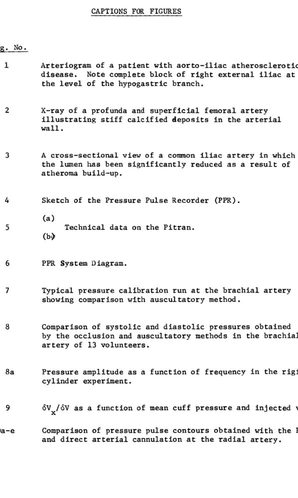
CAPTIONS FOR FIGURES 73
FIGURES (1-60) 78
APPENDIX A - Computer Listing (Al-A17) 79 APPENDIX B - % Area Reduction as a Function
of Clamp Opening 167
APPENDIX C - Electrical Drawings and Specifications
Page No.
MEDICAL GLOSSARY 172
REFERENCES 178
NOMENCLATURE
A cross-sectional area
A local area at reference pressure
BP brachial artery blood pressure (systolic/diastolic) BPM beats per minute (HR)
c pulse-wave velocity (wave speed) C segment volumetric compliance
CC control case
C compliance of arterial section surrounded by monitoring cuff (6V /6p a a)
Cu vessel compliance per unit length (DA/3P) CT volume compliance of tibial termination
D diameter
D clamp gap
Dco clamp gap (no obstruction)
f wall friction force per unit mass of blood
F approximate viscous coefficient in momentum equation GAIN PPR electrical gain
HR heartrate (BPM)
Hz hertz (cycles per second)
i time notation for finite difference method
k entrance loss coefficient
KHz 1000 hertz
L length of obstruction Ln(X) the natural log of X
Lu inertance per unit length (p/A 0)
N spatial notation for finite difference method
p pressure
p mean pressure
pATM atmospheric pressure
Pa arterial pressure
Pc absolute cuff pressure PCUFF cuff gage pressure (P
C
pO reference pressure
PPR pressure pulse recorder
Pv venous pressure
PS systolic pressure Q volume rate of flow
Q mean flow
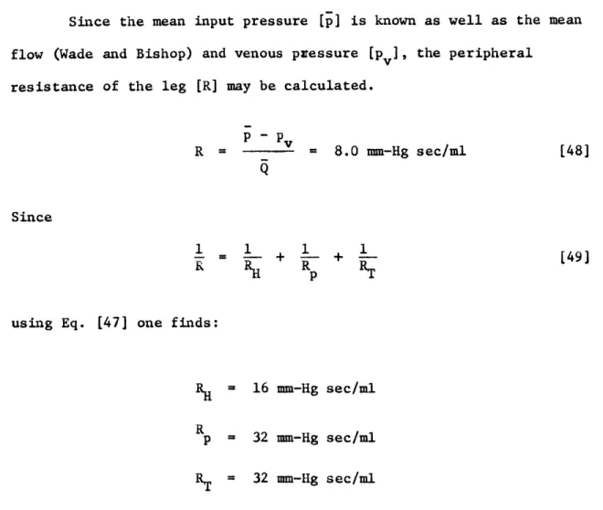
QL leakage term in continuity equation R leg peripheral resistance
R 1primary termination or branch resistance R2 secondary termination or branch resistance R H hypogastric resistance
R profunda resistance p
RPR real peripheral resistance
RT tibial resistance also (R + R2) for general representation
u mean fluid velocity (1 - D)
V volume of air in cuff monitoring circuit of PPR C
V injected volume
V tube volume from an internal shut-off valve in the PPR to the monitoring cuff
V2 tube volume from the shut-off valve in the PPR to
the syringe
x longitudinal distance
th th
denotes the value of X at the i time step and the N spatial step
z 0characteristic impedance ZT termination or load impedance
CL percent arterial area change per 50 mm-Hg at 100 mm-Hg proportionality constant relating p to C
u 6pc cuff pressure change
6V volume change applied to cuff 6V a arterial volume change
6V c cuff volume change
6V xvolume change due to the expansion of the bladder over a monitoring cycle
A relative amplitude of PPR traces AP pressure drop across obstruction
APBL pressure loss due to developing boundary layer in obstruction model
AP pressure loss due to contraction in obstruction
c model
APu pressure loss due to unsteady flow AP expansion pressure loss
At time step for finite difference method
Ax spatial element for finite difference method TI Womersley Frequency Parameter
Y ratio of specific heats
$ phase of reflection coefficient
P dynamic viscosity
v kinematic viscosity
w pulsatile or circular frequency
p fluid density
symbol used in the finite difference method
0 symbol used in the finite difference method
Arteriosclerosis is a term applied to a number of pathological conditions in which there is thickening, hardening, and loss of
elasticity of the arterial wall. Atherosclerosis is a form of arterio-sclerosis in 'Thich there are localized inflammatory lesions (atheromas) within or beneath the intimal surface of the arterial wall. This condition
is thought to be due to general arterial wear and metabolic defect involving lipids and lipoproteins (1,2) and is one of the common causes of arterial narrowing and occlusion.
Arteriosclerosis is present to some extent in almost all adults and can involve almost any artery, thus producing a variety of symptoms and consequences. The most common examples of acute conditions include:
i) myocardial infarction - a portion of the heart muscle becomes damaged because of interruption of its blood supply by atherosclerotic occlusion, acute thrombosis,
or coronary artery embolism.
ii) stroke - the blood supply to portions of the brain is suddenly reduced by cerebral arterial occlusion or embolus.
iii) gangrene - the blood supply to a peripheral tissue mass is reduced due to arterial occlusion and the tissue dies. More chronic conditions include angina, transient cerebral ischemia, and
intermittent claudication.
In the last ten years options open to physicians for the treatment of arteriosclerosis have increased at a rapid pace (3). Surgical
revas-cularization is now possible in an increasing number of anatomical areas ranging from the myocardium to the arteries of the lower limbs (4,5,6,7). This has been possible through the development of prosthetic grafts,
techniques involving the removal of atheroma, and the use of vein segments for arterial bypass (8). Drug and dietary treatment for high blood levels of cholesterol and triglyceride, as well as hypertension have also been expanded with success (9).
As these new procedures have become more common the need for early and accurate evaluation of arteriosclerosis has become more acute, both for the clinician and the research scientist.
Arteriography is the primary invasive technique for the diagnosis of arteriosclerosis in man. It is performed by injecting radio-opaque dye into an artery in the region of interest and taking roentgenograms of
the area. Figure 1 is an example of an arteriogram taken in a patient with aorto-iliac disease. The procedure consists of inserting 18 gauge needles in the common femoral arteries at the level of the inguinal ligament and injecting 35cc of Renograffin-60R into each artery just prior to X-ray. While this technique often provides the vascular surgeon with an arterial
"roadmap" there are a number of drawbacks:
i) The technique is expensive. It requires hospitalization and is performed either in the operating room or in an
elaborate radiology suite. Typically two physicians, a nurse, and an X-ray technician are required for an hour with an aggregate cost, including hospitalization, of
producing varying degrees of pain during and immediately following the dye injection. Many patients describe arteriography as more of an ordeal than the operation for which they are being examined. In addition, the dye may produce nausea and diuresis, and in some cases cannot be used due to allergy.
iii) Hazards of the procedure are not uncommon and include possible intimal damage to the artery at the site of puncture, local artery thrombosis, and hematoma in the region wiere surgery will be
performed.
iv) It is often quite difficult to interpret arteriograms (10). Even when arteriograms have been taken in
two orthogonal planes lumen obstruction and hemodynamic significance of the lesions are not clear.
v) The procedure cannot be performed repeatedly.
Since present non-invasive techniques have many shortcomings that will be outlined in a subsequent section of this paper, new non-invasive
techniques for preoperative evaluation, monitoring during arterial reconstruction, post-operative monitoring and assessment of arterial condition after and during drug and dietary treatment are needed.
The rationale we have adopted to develop a new non-invasive
conditions such as increased arterial wall stiffness by calcified deposits (Fig. 2) and decreased lumen area by atheromatous build-up (Fig. 3) which in turn change the pressure and flow characteristics of the arterial pulse. The effects of these pathological changes on the arterial pressure and flow pulses will be discussed with the aid of experimental and theoretical data.
In this investigation the diagnosis and analysis of peripheral vascular disease in the lower limbs were chosen as the focal points. This decision was made because of the prevalence of all forms of arteriosclerosis below the renal arteries (11) and because arteries of the lower limbs are accessible to different forms of diagnostic measurement.
The first task in the research was to develop a device, referred to here as a Pressure Pulse Recorder (PPR), that could be used non-invasively to measure the pressure pulse at specific sites on the lower
extremities. The second step was to study the pressure pulse characteristics recorded with the PPR in diseased and healthy arteries. In
accomplish-ing this, patients undergoaccomplish-ing vascular reconstruction were studied pre-operatively, intra-pre-operatively, post-operatively, and during office
follow-up examinations during an 18-month period. Results provided by the PPR were compared to arteriograms, surgical findings, and clinical information.
To aid in the interpretation of measurements made during the clinical studies a computer simulation of the arteries of the lower
was developed. The major requirement of the model was to accurately mimic the pulse propagation along the arteries. Relevant physiological
data were obtained and used in the model. When a control case
corresponding to a normal healthy individual was defined, the arterial elasticity, reflection coefficients, and other circulatory parameters were varied and their effects analyzed with the model. In addition
various degrees of obstruction were introduced in the simulated arteries. Verification of model results were obtained from human data and dog
experiments.
In summary, this report describes:
i) the development of an instrument to non-invasively record the pressure pulse on the lower extremities.
ii) the measurement of arterial pressure pulses in diseased and normal arteries. iii) the interpretation of observations of the
arterial pressure pulse by means of
II. PRESSURE PULSE RECORDER-DEVELOPMENT AND DESCRIPTION
The development of the PPR was prompted by the fact that no adequate non-invasive instrument was available for the measurement and recording of arterial pressure pulses in the extremities. 2.1 Current Non-Invasive Devices
The examination of a patient for an arterial abnormality generally includes symptomatology, pulse palpation, auscultation by stethoscope (bruit location), as well as observations such as limb pallor, temperature, and capillary filling.
In addition to the stethoscope as previously mentioned there are some other non-invasive instruments currently in use.
The oscillometer (12,13) is the oldest of the devices used specifically to aid in the diagnosis of vascular problems. It
consists of two small overlapping blood pressure cuffs and a mechanical pressure transducer. When its sensitivity is adequate, it provides a
qualitative indication of limb volume pulse with its output read on an aneroid gage. It is highly qualitative, cannot be standardized,
provides no contour information, provides no permanent record, and in most cases is not sensitive enough to distinguish all but the most
obvious peripheral vascular abnormalities. It is, however, easy to use and inexpensive.
In recent years the transcutaneous Doppler ultrasonic blood-velocity detector (14,15,16) has gained popularity among vascular
the presence of blood flow in arteries and can be used in conjunction with the cuff occlusion method to accurately measure systolic blood pressure in the lower limbs. With the Doppler velocity detector in
its present form it is virtually impossible to obtain transcutaneously any quantitative measurement of blood velocity because the angle
between the ultrasonic beam and the vessels is not known accurately and cannot be maintained.
Two other instruments deserve mention. They are the mercury-in-silastic strain gage (23,24) and the impedance segmental plethysmograph
(25). The mercury-in-silastic strain gage measures the change in limb or digit circumference. The impedance segmental plethysmograph measures impedance changes in a limb segment secondary to pulsatile blood
volume changes. Both of these devices do produce hardcopy readout and contour information, however, they cannot be standardized and produce traces with high noise content. For these reasons they are not of great use in diagnosis or in following the state of the peripheral vascular system.
2.2 The Pressure Pulse Recorder
The following sections describe an instrument that produces a reasonably accurate recording of the arterial pressure pulse at various sites on the extremities. This instrument records the segmental limb volume displacement due to the passage of the arterial pressure pulse. With the aid of some experimental work including in vivo simultaneous measurement of intra-arterial pressure and non-invasive pressure pulse
recordings an operating procedure was developed such that the pulsatile volume displacement is approximately proportional to the
arterial pressure pulse. The trace can be calibrated by two independent pressure measurements of systolic and diastolic pressure and the
instrument constitutes then an arterial pressure pulse recorder (PPR). For screening purposes the instrument is essentially used to compare the pressure pulse amplitudes recorded at different locations along the two legs (at the thigh, calf and ankle). If the amplitudes are different in the two legs, this is interpreted as the presence of an obstruction proximal to the monitoring site in the leg which has the smallest amplitude. A sharp amplitude drop in the same leg between two sites is also indicative of a block. For monitoring, a comparison of the pulse amplitudes recorded before and after revascularization provides a verification that surgery has improved peripheral circulation.
Although pulse amplitude by itself provides important information, it is logical to assume that additional information can be extracted from the entire pulse contour. For this reason, it is important that the recording represent as accurately as possible the true arterial pressure pulse. The accuracy of this instrument rests on an optimum design of the electronic components permitting a large amplification of the signal and the use of low cuff pressures.
2.3 Description and Operating Procedures
The PPR (Fig. 4) consists of two non-overlapping air-filled *
cuffs , one for pressure monitoring and the other for occluding the
artery for calibration purposes. These cuffs consist of a neoprene bladder (13 cm wide, 23 cm long) covered by a semi-rigid nylon-velcro band. When recordings are made at the thigh a larger cuff (18 cm wide,
35 cm long - bladder size) of the same material is used. The monitoring cuff is connected by stiff latex tubing to a pressure sensitive
transistor (Pitran - 0.1 psid series). The Pitran is a silicon IPN planar transistor with its emitter-base junction mechanically coupled
to a diaphragm. A differential pressure applied to the diaphragm produces a large, reversible change in the gain of the transistor which has a uniform frequency response up to 150 KH z. Figure 5 provides
additional technical data on the Pitran, while a diagram of the layout is represented on Fig. 6. The instrument is compact and self-contained and can be operated by paramedical personnel after a brief training period.
The other electronic components of the PPR are:
i) A sample-and-hold circuit operating in closed-loop fashion to maintain the proper operating point for the pressure sensor.
ii) Logic circuits to configure the 120 volt AC solenoid
*
valves according to the mode selected by the operator. iii) A dual-limit comparator to detect and correct for
excessive differential pressure applied to the sensor. iv) A panel switch to provide DC-coupled or AC-coupled
output to the chart recorder with a sensitivity selected by the operator.
v) A peak-to-peak detector to provide an indication
of relative pulse volume on the panel meter.
Detail electrical drawings and specifications are provided in Appendix C. This appendix was prepared by the Medical Engineering Company, Mansfield, Massachusetts.
Either cuff can be connected to an aneroid pressure gage which serves to measure the mean cuff pressure. A built-in syringe is used to introduce a definite volume of air at atmospheric pressure into the bladder of the cuff (generally 75 ml for the arm, ankle and calf cuff and 200 ml for the thigh cuff). The band around the bladder of the cuff is used to adjust the pressure in the monitoring cuff to a value sufficient to insure close contact with the skin, but well below
diastolic pressure. The proximal cuff is open to atmospheric pressure. The passage of the arterial pulse causes the segmental volume of the limb surrounded by the cuff to change. The changes in limb volume are absorbed by the bladder which is contained by the semi-rigid band. The
cuff pressure fluctuations caused by the cuff volume changes are trans-formed into electric signals by the transistor. The output signal is displayed on a convenient recording device (an ECG recorder is adequate).
2.4 Measurement of Systolic and Diastolic Pressure in the Lower Limbs To permit maximum use of the chart width and provide stable recordings, the instrument is AC-coupled with a time constant of 1 sec. As a result the pressure trace is centered on the chart and the
location of zero pressure is not known. It is therefore necessary to calibrate tlhe pressure scale by measuring independently the systolic and diastolic pressures at the site of the recording. This calibration
is made with an occlusion cuff placed proximally. A typical measurement of systolic and diastolic pressure with the PPR for the brachial
artery is shown in Fig. 7. The pressure in the occlusion cuff is raised above systolic pressure (no oscillations in the monitoring cuff) then is slowly lowered until the pressure in the monitoring cuff starts to fluctuate. The systolic pressure is read from the aneroid gage at the onset of the pressure fluctuations in the monitoring cuff. As the
pressure is lowered in the occluding cuff the oscillations in the monitor-ing cuff grow in amplitude and generally overshoot the control value obtained when the pressure in the occluding cuff was zero. At the
point the oscillations reach a maximum diastolic pressure is read as the pressure in the occluding cuff. Although the cuff pressure at which oscillations reach their maximum amplitude does not rigorously correspond to the diastolic pressure, a study illustrated in Fig. 8 has indicated that it provides a convenient and reasonably criterion for diastolic pressure especially if the venous return is not interrupted for a long period. This figure gives a comparison of systolic and diastolic pressures obtained by the occlusion and auscultatory methods in the brachial arteries of 13 healthy volunteers using standard blood pressure cuffs 13 cm in width. As suggested by Karvonen et al. (26) the diastolic pressures indicated by the auscultatory method have been decreased by
7-8 mm-Hg. This correction generally brings the diastolic pressure in closer agreement with those indicated by the PPR. The systolic pressures determined by the PPR are consistently higher than those obtained by the auscultatory method, but the difference is small. Systolic and diastolic pressures obtained by the PPR have also been compared with pressures measured by cannulation of the radial and common femoral arteries at
surgery and during arteriography, respectively. The agreement was very similar to that presented in Fig. 8.
2.5 Dynamics of the Air in the Cuff
To aid in the development of the PPR operating procedure and the interpretation of its recordings it was important to understand how the pressure of the air in the cuff related to the arterial pressure. In order to accomplish this a number of experiments were performed in addition to analysis.
First, consider the constant mass of air in the cuff at an
absolute pressure p c in a volume V . Further, if it is assumed that the gas undergoes an isentropic process the following equation may be written
p V = const [1]
where y is the ratio of specific heats (for air, y = 1.4).
To test the validity of the isentropic assumption the pressure measuring components of the PPR were connected to a rigid cylinder (50 ml volume). Also included in the pneumatic circuit was a small piston-in-cylinder pump with a 1 ml stroke volume. The pump was used to oscillate
the total volume of the system at various frequencies while measuring the pressure changes. It was found that at frequencies from 0.25 Hz to 20 Hz (highest frequency tested) the pressure amplitude remained constant. The
*
frequency (isothermal) to 0.25 Hz. This experiment suggests that in the range of frequencies encountered in clinical use (0.50 to 1.5 Hz) the
air in the cuff undergoes an isentropic process, changing from isothermal to isentropic between zero and 0.25 Hz. The heat transfer characteristics of the bladder may be different than the rigid cylinder due to geometry and material differences. This is discussed in a later section. Also, it will be shown later that the identification of the process is not critical
to the analysis as its effect is to be combined with the elastic expansion of the cuff. Since the volume excursions in the cuff are a small fraction
(2% max) of its mean volume, Eq. [1] can be differentiated to give
6p = c 6V [2]
6V
c - c
C
where p c and Vc have been replaced by their time-mean values PC and V respectively. The time-mean volume V is also a function of
cuff pressure and the injected air mass. If the initial volume of air injected at atmospheric pressure (pATM) is V1 , the volume of air in the cuff is defined by Eq. [3]
- ATM (V + V + V2 2 [3]
Here V is the tube volume from an internal shut-off valve in the PPR to the monitoring cuff; V2 represents the tube volume from the shut-off valve
to the syringe. In the prototype built V1 and V2 are 21 and 22 cc, respectively. The compression of the injected air is assumed to be iso-thermal since it subsists for a long period of time, much longer than 4 sec
(0.25 Hz).
*
Combining Eqs. [2] and [3] we find
- y6V 12
6pC = c C [4]
(p ~ATMC (V + V1 +V) - V 2 )
To investigate the validity of Eq. [4] another experiment was performed. The monitoring cuff was connected to the PPR electronics with a 1.0 ml syringe also in the pneumatic circuit. The syringe was used to change the total air volume in increments of 0.25 ml from
0.25 ml to 1.0 ml at different cuff pressures and initial injected
volumes. Cuff gage pressures of 20,40,60,80 and 100 mm-Hg were used with injected volumes of 25,50,75 and 100 ml. The results of this experiment indicated that the bladder constrained by the nylon-velero band is
not inextensible, but instead expands with pressure over a monitoring cycle. The edges and corners of the bladder which are not constrained by the cuff may move and make additional volume available. The actual volume change of the air in the bladder 6V is calculated from the measured pressure change using Eq. [4]. Then the volume 6V due to the expansion of the cuff is defined by
6V = 6V - 6V [5]
x
c
where 6V is the volume change applied to the cuff.
Figure 9 illustrates how the ratio 6V /6V varies with mean cuff pressures and injected volumes. It is interesting to note that the extrapolation of the measurements to p + 0 leads to 6V
c
= 6Vand that even at high cuff pressures the expansion is still present, but to a lesser degree as the bladder becomes stiffer. The fact that wrapping an inextensible band around the cuff does not change the results suggests that end effects, not the stretching of the bladder,
is the dominant factor. This observation suggests that the sensitivity of the instrument may be considerably improved by designing a cuff which
absorbs all the limb volume change. Including the results of the preceding experiment we rewrite Eq. [4] as
6V -y6V(l - x
OC C (PATi4'c (VI + V1 + V2 - 2) [6]
[
]
The next step in the analysis is to assume that the volume changes of the limb caused by tae passage of the pressure pulse are proportional to the changes in the arterial volume 6Va encompassed by the cuff. We write
6V = 6V = C 6 p [7]
a a a
where C = 6V a/6p is the compliance of the arterial section a a a
surrounded by the cuff and pa denotes the arterial pressure. Combining Eqs. [6] and [7]
6V
YCa6pa(
6p = a a [8]
( ATM c (VI+ V +V2 2
Since 6V /6V is approximately independent of 6V , it follows from
Eq. [8] that if Ca remains constant the variations in the cuff
pressure are proportional to the variations in arterial pressure and the output of the pressure sensitive transistor will yield a good representation of the arterial pulse contour. The critical experiment
to test the accuracy of this analysis is of course the comparison with
direct intra-arterial measurements.
2.6 Comparisons with Intra-Arterial Measurements
To verify the accuracy of tue pressure pulse contours produced by the PPR, recordings were compared with direct intra-arterial pressure measurements taken at the same location. Five comparisons on different subjects prior to surgery were performed by placing the PPR monitoring cuff around the forearm while simultaneously recording radial artery pressure with a cannula (the radial cannula had been placed for
surgical monitoring purposes). The transducer used for all the direct
pressure measurements was a Hewlett Packard Model 267 BC. The cannula
was an 18 gauge needle connected to a 2 foot length of rigid wall catheter. All comparisons yielded the same degree of agreement, even
though patient size, weight, and age were in general different. Figures lOa-lOe show comparisons made at the radial artery with recordings taken
externally in the same arm with various adjustments of the mean cuff pressure. Only the recordings for 30 (lowest value for good bladder contact) and 100 mm-Hg are shown as the traces corresponding to inter-mediate values fall between these two limiting curves. Since the
drawn and scaled to the same amplitude. Five additional comparisons were made during arteriography with the PPR monitoring cuff placed high on the thigh while simultaneously recording common femoral artery pressure via a cannula. In all cases, no arterial block was present in the short distance between the cannula and the cuff. Figures lla-lle illustrate comparisons taken at the thigh after appropriate scaling. Further studies at the calf were made during arterial reconstruction by introducing a catheter down the popliteal artery. The results showing identical trends as illustrated by Figs. 10 and 11.
The results of our studies indicate that the smaller the cuff pressure, the closer the PPR recording is to the true pressure contour. We postulate, since the presence of the cuff reduces the transmural
pressure in the artery beneath it, at high cuff pressure, the nonlinearity of the arterial pressure-volume relationship (27) produces a marked
distortion in the recorded pulse contour. The distortion is proportionally larger in the diastolic part of the pulse. Viscoelastic effects present
in the tissue and arterial wall also probably distort the PPR traces. However, the cuff pressure must be sufficient to produce adequate contact between the bladder and the skin. A cuff pressure of 30 mm-Hg provides good bladder contact and still gives a reasonably good agree-ment with intra-arterial measureagree-ments.
In another study we changed injected volume while holding cuff pressure constant over a range of 20 ml to 125 ml. The results indicate
that the injected volume in the cuff does not alter significantly the pressure pulse contour [see Fig. 12] and that the injected volume in the
cuff may be lowered as low as 20cc if a larger signal is desired without danger of distorting the pulse contour.
2.7 Frequency Response
The frequency response of the complete device (cuff and
electronic circuit) was tested by connecting a liquid-filled bladder to a small piston-in-cylinder pump producing a sinusoidal change in volume in the bladder. This bladder was strapped around a rigid plastic cylinder and surrounded by the air-filled monitoring cuff of the device. The action of the pump produced oscillations in the volume, and consequently in the pressure of the monitoring cuff. The amplitude of the air pressure oscillations in the cuff remained constant from 0.25 Hz to 20 Hz (as in the rigid cylinder experiment). The
natural frequency of the cuff and electronic system was determined to be approximately 55 Hz by sharply tapping tae monitoring cuff and measuring the frequency of the vibration from the trace (28). Two important conclusions may be drawn from these observations. First, the frequency response is sufficient for monitoring the pressure pulse since a frequency response of 20 Hz is considered to be adequate (29).
Secondly, we have an experimental confirmation of the assumption that the pressure pulse compresses the cuff isentropically. If the
compression was isothermal (or at least non-adiabatic) at the usual
heart frequency, it would certainly become adiabatic at higher frequencies (between 0.25 and 20 Hz) when the duration of each cycle is too small for
heat transfer to occur. If this was the case the change in the coefficient y in Eq. [2] (from 1 for isothermal compression to 1.4 for adiabatic compression) would cause a 40% increase in cuff pressure amplitude over the frequency range.
In summary, it has been established that the readings produced by the PPR are reasonably close to the actual arterial pulse contour if the pressure in the cuff is at 30 mm-Hg or below.
Sample recordings taken at the brachial artery, forearm, thigh, calf, and ankle of both upper and lower extremities in a healthy
III. CLINICAL STUDIES AND OBSERVATIONS
Two Pressure Pulse Recorders were constructed and tested at the Fluid Mechanics Laboratory at M.I.T. The conceptual design and general construction were performed by the author. The electronic circuits were built by the Medical Engineering Company of Mansfield, Massachusetts. When the units had undergone sufficient laboratory testing they were transferred to the Massachusetts General Hospital. One unit was placed
in the office of R. Clement Darling, M.D., for initial patient evaluation and follow-up. The other unit remained in the hospital to be used for
in-patient pre-operative, intra-operative, and post-operative studies. The plan included studying as many patients as possible undergoing vascular reconstruction and comparing data obtained with the PPR with results from current methods. In the course of an 18-month period over
200 patients were examined with the PPR. The clinical PPR examinations include:
i) the measurement of systolic blood pressure at the brachial artery, thigh, calf, and ankle at rest in all extremities.
ii) recordings of thigh, calf, and ankle pressure pulse contours in both legs at rest.
iii) noting the presence or absence of femoral, popliteal, and pedal pulses.
iv) patients were asked to walk at their normal rate until claudication occurred or 200 yards
taken at the ankle; the maximum walking time and character of the recordings and pressures after exercise were measured
(a treadmill is now being used).
v) other pertinent clinical information was recorded such as absence or presence of rubor and bruits, as well as, limb skin temperature.
A wide spectrum of vascular disease was encountered: aneurysmal and occlusive disease of the aorta and distal vessels, vasospastic disease, and occlusive disease of the upper and lower extremities. The
following cases are given to illustrate how the PPR data were used, and how they correlated with the clinical and angiographic findings.
3.1 Case Studies
The first case was a 50 year old female (YW) presented with sudden onset of claudication of the right calf radiating to the thigh. All pulses were palpable in both lower extremities. Figure 14 is a comparison of the angiographic findings and the resting pre-operative PPR examination. On the right side the pulse amplitudes [A] were
severely reduced despite palpable pulses at rest. A 60 mm-Hg systolic pressure difference (measured with the PPR using the occlusion method) was present between the brachial artery and the right femoral artery.
on the right side after walking 150 yards in 1.5 minutes. Figure 15 shows the pulse amplitude at the right ankle became flat and required
2.5 minutes after ceasing exercise before returning to the normal
resting level. The pulse amplitude at the left ankle actually increased after exercise and returned to normal after a short period of time. Figure 16 shows that, after insertion of an aortoiliac bifurcation graft, the pulse amplitude in the lower extremities were equal. In addition, no pressure difference in systolic pressure between upper and
lower extremities could be demonstrated. Figure 17 shows that, post-operatively, after exercise no diminution in pulse amplitudes at the ankles were present. Actually the pulse amplitudes in the ankles increased twofold with exercise.
The second case [KN] was a 65 year old stockbroker, a heavy smoker, and diabetic for 25 years. He presented a long history of bilateral calf claudication and threatened gangrene of toes on the right
foot. Good femoral pulses were the only pulses palpable. Pre-operative findings are presented in Fig. 18. The PPR examination suggested severe ischemia on the right side with a 70 mm-Hg difference in systolic
pressure between the brachial artery (left arm) and the superficial femoral arteries in both legs. The patient was not asked to exercise because of the threatened gangrene of the right foot. The diagnosis of bilateral superficial femoral occlusion with tibial vessel involvement was made and confirmed by arteriogram. Figure 19 illustrates the findings
vein bypass graft in the right leg. No vascular reconstruction was performed in the left leg. The pulse amplitude increase on the right side is evident by examining pre- and post-operative traces (Figs. 18 and 19). In addition, the systolic pressure differences between the brachial artery and the superficial femoral artery on the right side was reduced from 70 mm-Hg to 10 mm-Hg. Figure 20 shows the results after walking the patient 100 yards in 2.5 minutes. Note the left ankle pulse amplitude goes to zero and requires three minutes to return
to normal. Following surgery claudication was no longer present at the right calf.
The object of the third case is to emphasize the application of monitoring with the PPR during vascular reconstruction. The patient
(TB) was a 62 year old male, ex-smoker presented with a 10 cm abdominal aortic aneurysm, right superficial femoral occlusion, and left iliac obstruction secondary to the aneurysm. Prior to surgical preparation, blood pressure cuffs used with the PPR were placed at the calf level of both legs. At the beginning of surgery, readings were taken at the right and left calves (the device is placed at a convenient location in the operating room and the air hose from the cuffs connected to the
electronics). These pre-operative readings along with the remaining read-ings of this study are given in Fig. 21. With the aneurysm resected and the left anastomosis completed, a recording was taken as the clamp was removed from the left iliac limb. At this point, as illustrated, a 33 mm relative pressure pulse amplitude was recorded at the left calf. When the right anastomosis was completed and the clamp removed, the pulse amplitude remained zero at the calf although the pre-operative recording was 8mm. A good femoral pulse, however, could be felt on the operating table. Due to the
superficial femoral artery occlusion no palpable pulses were expected below the femoral level after surgery. The PPR provided a non-invasive method of immediately evaluating the reconstruction. The common
femoral was explored and a thrombus removed at the profunda femoris level. When this was completed the recorded amplitude at the right calf was 10 mm. The remainder of the procedure was uneventful and angiography was notnecessary.
In addition to the frequent vascular conditions previously described the PPR was used in other less common clinical situations. PPR examinations were requested by the Pediatric Service for two infants because of suspected coarctation of the aorta (conventional blood pressure measurements had not proved useful). In the first case a 50 mm-Hg
systolic pressure difference between the upper and lower limbs confirmed the diagnosis, and further study was warranted. In the second case no systolic difference was present and the child was discharged. In three cases involving the catheterization of very young children the PPR was used to look for the complication of femoral artery thrombosis. When the examinations proved positive, thrombectomy was performed in all three cases. The device was used for intra-operative monitoring and post-operative follow-up as well. In one case the thrombectomy was not
successful and the child was examined at regular intervals over a two week period and released when the device indicated adequate collateral circula-tion had developed. In two cases the PPR was used for verification of thoracic outlet syndrome. Angiography had not proven decisive in either case. In one case the syndrome was convincingly demonstrated by near
zero PPR amplitudes when the patient extended her neck and arms to the point of pain. In the other case no arterial changes occurred with position, the symptoms later found to be of neurological origin only.
During the clinical evaluation period the PPR was demonstrated to be consistent in the monitoring of arterial pressure as shown by the following examples.
A patient (RS) was examined four times with the PPR over a
nine month period. he was followed for general atherosclerotic disease after a carotid endarterectomy was performed. Figure 22 illustrates the PPR traces at the left calf using the same cuff pressures and volumes during the period of study. The consistency of the PPR traces
is confirmed by the patient's clinical evaluation regarding the peripheral arterial system of the lower limbs. It is important to note that the PPR traces were not affected by seasonal temperature
variations. All recordings were taken in a standard examination room with no special temperature control.
A patient (JA) was examined seven times with the PPR over a
twelve month period following insertion of an aorto-femoral bypass graft (Fig. 23). On the fourth visit it was found that the left limb of the graft had occluded. The amount of collateral circulation after occlusion may also be assessed from these traces.
In a series of seven patients in which one extremity (upper or lower) was grossly enlarged while the extremity on the other side remained normal in the absence of arterial disease on either side, it was concluded that, when properly applied the PPR will produce virtually
identical traces on the left and right limbs. An example is patient (BH) who developed lymphedema of the left arm following an automobile accident. The circumference of her left upper arm was twice tnat of the right arm. Figure 24 shows that recordings taken at the left and right brachial artery at the same cuff pressure and injected volume are almost identical. From this series of patients we concluded that edematous tissue does not appreciatively alter the contour or
amplitude of the PPR recordings. 3.2 Pressure Pulse Contours
In addition to pressure pulse amplitude changes, there are distinct alterations in the pressure pulse contour with peripheral vascular disease. Figure 25 shows recordings taken at the right calf
of three healthy athletic young men. Note the sharp rise and fall of the pulse during the initial phase followed by a distinct wave in the latter half of the trace. For reasons to be explained later this wave will be referred to as a reflected wave.
Figure 26 presents recordings taken at the right and left ankles of a 50 year old male (WP). This patient had an occlusion of the left superficial femoral artery and complained of claudication at 50 yards. His right leg was asymptomatic and the corresponding ankle recording was relatively normal. At the left ankle the systolic pressure was reduced by 15 mm-Hg, in addition this contour is considerably different. The upstroke was sharp, however, the descending phase of the curve was slow and the reflected wave was absent.
Figure 27 illustrates recordings taken at the right and left calves of a 30 year old female (MM). This patient had a long standing right common femoral artery thrombosis which was caused as a result of a left heart catheterization. Te left femoral artery was normal. Right calf claudication was present after walking 100 yards and pain radiated to the thigh with continued exertion. The contour changes seen in this case are similar to the changes observed in the preceding case.
It is beyond the scope of this work to make a detailed analysis of all the parameters and situations that have been dealt with during
the clinical studies. However, regarding the contour of the pressure pulse, certain changes deserve attention. In all cases when significant occlusive disease was present a reflected wave was never observed distal to the obstruction. Instead, traces similar to those of tne symptomatic side in Figs. 26 and 27 were found. In older persons the reflected wave was often not present, however, in these cases when the vessels were open a rapid rise was noted along with an exponential pressure decay. This
is in contrast to the patient with arterial occlusion where the rate of pressure rise distal to occlusion is reduced and the pressure decay slow.
Blood pressure levels and palpable pulses are often normal at rest in patients with significant peripheral vascular disease; in this case the only indication of an abnormality at rest is the shape of the pressure pulse contour. However, if significant occlusive disease is present the muscle mass distal to an obstruction will not be adequately perfused when the patient exercises. This inadequate perfusion causes claudication and
pressure reduction. This pressure reduction (both mean and pulse pressure) results in decreased recordings distal to the muscle mass as demonstrated in Figs. 15 and 20. To determine what happens to the recordings in the normal individual with exercise, healthy athletes were examined before and after running. Typical results are presented
in Fig. 28. The recorded amplitude increases with exercise and returns to normal shortly after ceasing exercise. In addition, the reflected wave is no longer present directly after exercise, but returns with
time. Post-exercise examination with the PPR is helpful in monitoring the state of the peripheral vascular system under stress.
In summary, the PPR traces provide consistent information with regard to the state of the peripheral vascular system, and can be
used to follow patients over extended periods of time. PPR recordings taken after exercise may reveal vascular abnormalities that would not be detected in the resting state. In addition, the device has been most
helpful for intra-operative monitoring during vascular reconstruction (30). Finally, arterial occlusions can be detected by contour and amplitude
IV. kATHEMATICAL MODEL OF ARTERIAL FLOW
Since the pioneering work of Frank (31) in 1899, numerous electrical, mechanical and computer simulations of the arterial system have been attempted, all aimed at a better understanding of
cardiovascular dynamics. An extensive survey of mathematical models is given by Noordergraaf (32). Lost of these simulations require that some restrictions be placed on the geometric and elastic properties of the arterial system as required by the electrical components them-selves or by linearization of the equations of a computational model. This section presents a convenient and economical method of calculation, based on a finite difference technique, for a one-dimensional pulsatile flow in a network of elastic tubes naving arbitrary geometric and elastic properties. As more data on the dimensions and the compliance of
arteries become available this method makes possible more realistic and more accurate models of the arterial system than can be done with
electrical and other linearized models.
Our own observations reported in Cnapter 3, as well as those of otilers (33,34) have shown that a patient afflicted with severe vascular disease has a peripheral pressure pulse markedly different from tnat of a healthy person. The ultimate goal of the arterial model and method of calculation described in this section is to aid in the diagnosis of peripheral vascular diseases such as thrombosis and atherosclerotic
plaque formation, starting from observations of the shape of the pressure pulse contour, such as those taken with the PPR.
In order to be able to make accurate diagnoses from computed pressure pulse contours these contours must be free from artifacts resulting from the model itself or from the computational techniques used. Therefore the choice of the model, its degree of complexity, and the computational scheme of solution, are all crucial to the method. The model cannot reproduce the complete arterial tree, not only because the mathematical complexity and the computation time would be enormous, but also because physiologic data on arteries are still too limited to permit a model of great detail.
It
is clear tnat a compromise mustbe
sought and tnat the different options availaule for describing the blood flow and tue arterial tree must be tried and compared against each other in order to arrive at the simplest model which still describes reliably the shape of tne pressure pulse as it propagates into the peripheral arteries.The arterial models proposed in the past have ranged from electrical analogues made of lumped elements to elaborate mathematical models with continuously distributed properties. The lumped-element models are adequate for studying the relations between cardiac output
and peripheral load, but, because of the small number of lumped-elements present, they cannot mimic the high frequency behavior of the cardio-vascular system. An important step towards more versatile and more
realistic models was the discovery that the linearized one-dimensional equations of a flow in an elastic tube are formally identical to the telegraph equations [Landes (35]; thus the theoretical literature of electrical engineering on transmission lines could be immediately applied to the dynamics of the arterial system.
Although the models based on the transmission line analogy can be made to yield a qualitatively correct behavior of the pressure pulse, they all possess intrinsic limitations due to their linearity.
On tiie contrary, the fluid mechanical equations are nonlinear because of the term for the convective fluid acceleration in the equations of motion, and, even more importantly, because of the dependence of the
compliance and cross section on pressure. Solutions to the nonlinear equations for certain physiological states can be drastically different from solutions of the same equations once they are linearized. This has been illustrated by Miickisz (36) and in recent papers by Rockwell
(37) and Raines et al. (38).
4.1 Governing System of Equations
In this analysis, tne pressure and velocity are assumed to be uniform over the entire arterial cross section. This is an approximation to real arterial flow and means that we are considering spatial
average values of thIe dependent flow variables at each cross section. In making this assumption it is implied that the boundary layers are thin and that the streamlines are almost straight. We must, therefore, exclude small arteries as well as those with bends or rapid changes in
cross section. In pulsatile flow the thickness of the boundary layer is related to the Womersley Frequency parameter [n] (39).
D[]
T = R ,o/ [wl' 9]
where V is the kinematic viscosity of blood and w is the pulsatile frequency. The thickness of the boundary layer is of the order D/r .
In the arteries of the lower extremities nl is approximately 7. The stream-lines are relatively straight in the lower extremities because the area taper is gradual and sharp bends are not present to produce secondary flows. Westerhof et al. (40), Jager (41,42) and Noordergraaf (43)
have
analyzed the limitations of this assumption and have found it to be in accord with experimental results.The continuity and momentum equations for a one-dimensional flow in a flexible tube are, respectively,
-- +0 [10]
Dx t
_ t x P ax
Here u denotes the one-dimensional mean fluid velocity, A the tube cross sectional area, p the fluid density, p the pressure, and
Q [
= uA] the volume rate of flow; x is the longitudinal distance along the vessel and t denotes time. The symbol f represents the wall friction force per unit mass of fluid and will be explained later.On multiplying Eq. [10] by u and Eq. [11] by A , and adding the resulting equations, we obtain
aQ -- += + (Q 2/A) - A - lp+ + fA [12]12
at ax P ax
Equation [12] will be used instead of [11] as the momentum equation in this analysis. The system of governing equations is completed by
the "equation of state" of the vessel, which we assume to be represented in the form
A A(p,x) [13]
Note that Eq. [13] allows the vessel to be tapered and distended in
an arbitrary way by the transmural pressure, but excludes active muscular contraction of the vessel wall, relaxation effects, wall
inertia, and viscoelasticity. Attinger (44) and Westerhof (45) nave shown experimentally and theoretically, respectively, that these effects do not play a significant role in arterial dynamics. However, other
investigators are currently developing models including these effects (46).
4.2 Linearized Equations
Equation [11] is non-linear in two respects: (i) because of the quadratic term in Q , and (ii) because of the pressure dependence of A This equation has been linearized by several authors (40,47,48) by
assuming that the cross sectional area is a linear function of pressure and also that changes in area are relatively small, that is
(P - P) Cu(x) << A (x) [14]
where
A(x,p) A (x) + (p - p ) C (x)
Here C u= A/ap is the vessel compliance per unit length and A (x)
u t
quadratic term in Q is neglected in Eq. [12], Eqs. [10] and [12] may be written in linearized form as
+Q C
Cx)
= 0 [15]ax u at
+ L (x) DQ f [16]
ax u at
Here Lu (x) p/A (x) is the inertance per unit length of the fluid. Equations [15] and [16] show the well-known analogy with transmission lines with the corresponding quantities being: Q , electric current; p , electric potential; Cu , capacitance per unit length; Lu $
inductance per unit length; f , electric resistance per unit length. From the same analogy the local "characteristic impedance" of the vessel is defined as
pf + jL (x)W 1/2
Z (x) = (. u
o jC (x)[
where
j
H rl and w is the circular frequency (w = 120i/HR).In all studies performed in this report non-linear features were retained. However, the electrical analogy, although it is strictly valid only in the linearized case, proves especially useful for obtaining
insight into the treatment of boundary conditions. 4.3 Boundary Conditions
Proximal Boundary Condition
The proximal boundary condition (closest to the heart) may be set by giving either the flow or the pressure distribution as a
function of time. Here we consider only a periodic boundary condition, although the calculational method works as well with arbitrary time functions.
Distal Boundary Condition
In order to reduce the complexity, small arteries, arterioles and capillaries are generally not represented in detail in arterial models. Rather, it is customary to truncate the arterial tree at some point and to replace the remaining part by a lumped pure resistance. As seen from the electrical analogy reflected waves will occur at a termination point when the terminal arterial characteristic impedance does not match the local peripheral impedance. If this mismatch is present the steady-state component of the response to a sinusoidal
driving function will not be a simple travelling-wave pair of voltage and current (pressure and flow). It will be a more complicated function, which may be resolved mathematically into the sum of two oppositely moving sinusoidal travelling-wave pairs; the incident and the reflected waves. The reflection coefficient is defined as the ratio of magnitudes of the reflected waves and incident waves. Since reflected waves are observed to some extent physiologically (49,50,51), a practical scheme
should be developed for arterial models in which the magnitude of the reflection coefficient [K] is a parameter. The electrical analogy gives a clue as to how this may be accomplished. The reflection coefficient
at the end of a transmission line is (52)
zT - Z
K =
z
[18]where Z is the characteristic impedance and ZT is the load impedance. Many previous investigators (40,48) have set ZT = z0 in their arterial models. This produces no reflected waves and
there-fore is not realistic in the regions where reflected waves are important or when anatomical accuracy is desired.
In this study a distal boundary 'condition is employed which provides realistic values for the reflection coefficients while
retaining the physiological values of characteristic impedance and blood flow. In the small arteries forming transition between the large
arteries and the arterioles the resistance to the flow increases
progressively as the arterial diameter decreases. At the same time the coupling between vessel compliance and the frictional resistance helps damp out the large reflections as in acoustic mufflers. This is
presumably the reason why large high frequency reflections are not
observed in the normal human arterial system. Thus it is essential that at least some distensibility of the small vessels and vascular bed past the point of truncation be accounted for in the distal boundary condition. The simplest manner in which this can be done is to terminate the model of the artery at the truncation by a lumped compliance in parallel between two lumped resistances. The equivalent electrical network is represented in Fig. 29a. With this model the complex load impedance
is given by
Z =R + 2(1 jR2CTw) [19]
T 1 R 22+ 2C 2 2+RZT
The sum of the resistances is taken to be equal to the terminal resistance which is obtained from the known mean flowrate and mean pressure at the point of termination.
Conditions at Branching
Another set of boundary conditions is given at a bifurcation [see Fig. 29b]. The conservation of volume flow requires that
Q, = Q2 +3 . Since the mean velocities in the three branches are in general different, the pressures will also be different, according to Bernouilli's equation. However, because the dynamic pressure of blood
(-~ 2 mm-Hg) in large arteries represents a small fraction of the un-steady pressure amplitude (~ 50 mm-Hg), the pressures at points 1, 2
and 3 may be considered equal to a good approximation. 4.4 Friction Term
It is convenient to express the friction force per unit mass f in Eq. [12] as
2
f = FQ/pA [20]
In the equations that follow the viscous coefficient F depends on the assumptions made for the viscous effects. If they are neglected F = 0 . For Poiseuille flow, F = 8wp , where p is the dynamic
viscosity of blood. To obtain an approximate expression for the viscous effects in this study the coefficient derived from Poiseuille flow was used. This friction term is not very accurate for pulsatile flow in arteries but, since, the viscous pressure drops represents a small