HAL Id: hal-00317679
https://hal.archives-ouvertes.fr/hal-00317679
Submitted on 3 Nov 2004
HAL is a multi-disciplinary open access
archive for the deposit and dissemination of
sci-entific research documents, whether they are
pub-lished or not. The documents may come from
teaching and research institutions in France or
abroad, or from public or private research centers.
L’archive ouverte pluridisciplinaire HAL, est
destinée au dépôt et à la diffusion de documents
scientifiques de niveau recherche, publiés ou non,
émanant des établissements d’enseignement et de
recherche français ou étrangers, des laboratoires
publics ou privés.
patches in the morning sector
R. A. Makarevitch, F. Honary, I. W. Mccrea, V. S. C. Howells
To cite this version:
R. A. Makarevitch, F. Honary, I. W. Mccrea, V. S. C. Howells. Imaging riometer observations of
drifting absorption patches in the morning sector. Annales Geophysicae, European Geosciences Union,
2004, 22 (10), pp.3461-3478. �hal-00317679�
© European Geosciences Union 2004
Geophysicae
Imaging riometer observations of drifting absorption patches in the
morning sector
R. A. Makarevitch1, F. Honary1, I. W. McCrea2, and V. S. C. Howells2
1Department of Communication Systems, Lancaster University, Lancaster, LA1 4YR, UK 2Rutherford Appleton Laboratory, Chilton, Didcot, OX11 0QX, UK
Received: 10 December 2003 – Revised: 30 June 2004 – Accepted: 2 July 2004 – Published: 3 November 2004
Abstract. Observations by a 7×7-beam imaging riometer in Kilpisj¨arvi, Finland (∼66◦ MLAT) of the drifting cos-mic noise absorption (CNA) structures in the morning sector near the zonal drift reversals are presented. The examina-tion of the absorpexamina-tion intensity images revealed several re-gions with enhanced CNA (absorption patches) slowly drift-ing through the riometer field of view (FoV). The absorption patches were found to vary in shape, orientation (for elon-gated arc-like patches), and drift direction. The latter was calculated from the regression lines to positions of the ab-sorption maxima in the FoV images and compared with the direction of electrojet plasma flow from horizontal magnetic perturbations and (for one event) tristatic ion drift velocities in the F-region. A reasonable agreement was found between these directions both in point-by-point comparisons and in terms of direction reversal timings. The absorption patches of lower intensity appear to have smaller drift velocities and to be associated with weaker magnetic perturbations. These results are consistent with the notion that relatively slow mo-tions of the auroral absorption near the zonal drift reversals are associated with the E×B drift of the entire magnetic flux tube as opposed to the gradient-curvature drift of energetic electrons injected into the ionosphere at the substorm onset. The absorption drift velocity magnitude, on the other hand, was found to be substantially lower than that of the plasma flow based on the results of limited comparison with tristatic ion drift measurements. A comparison of the drift directions with those of the patch elongation showed that a consider-able number of patches had these directions close to each other. Using this observation, we demonstrate a satisfactory agreement between the patch drift velocities (both in direc-tion and magnitude) as determined from the absorpdirec-tion im-ages and keograms under the assumption that some patches were propagating in a direction that was significantly differ-ent from the perpendicularity to elongation.
Key words. Ionosphere (auroral ionosphere; electric fields and currents; plasma convection)
Correspondence to: R. A. Makarevitch
(r. makarevitch@lancaster.ac.uk)
1 Introduction
The spatial resolution of riometer systems has been gradually increasing over the years of research from several hundred (widebeam riometer sets) to a few tens of kilometers (imag-ing riometers), which has significantly extended the range of detectable absorption structures and enabled more accurate determination of the cosmic noise absorption (CNA) drift ve-locity (e.g. Hargreaves, 1970; Berkey et al., 1974; Nielsen, 1980; Kikuchi et al., 1990; Stauning et al., 1995; Kainuma et al., 2001; del Pozo et al., 2002, and references therein).
Berkey et al. (1974), by considering a large number of syn-optic absorption maps from over 40 riometer stations in the subauroral, auroral, and polar cap latitudes during substorm conditions, concluded that the absorption maxima in most cases moved eastward from the substorm injection area with a velocity of 0.7–7 km/s, consistent with the idea that the mo-tion of auroral particles injected during the substorm into the nightside ionosphere is governed by gradient-curvature (GC) drift. Hargreaves (1970), using the absorption data from 4 closely-spaced riometers, found a significantly lower (from 80 m/s to 3.3 km/s) range of velocities of eastward expan-sion with a significant number of absorption events expand-ing westward. This casted doubt on the validity of a simple injection-drift model and suggested that another mechanism could be responsible for the observed drifts of absorption fea-tures. Hargreaves (1970) proposed that the precipitating elec-trons are moving together with the entire magnetic flux tube and hence their motion is governed by the E×B drift or, in other words, by the high-latitude convection.
Later Nielsen (1980) in a four-narrow-beam riometer ex-periment in Northern Scandinavia studied the dynamics of absorption spikes during the substorm expansion phase and discovered that the spike velocity appeared to be different from the E×B drift velocity. Moreover, a comparison with the STARE radar measurements showed an almost ideal co-incidence over the observed range from 0.3 to 3.0 km/s be-tween the spike velocity and the velocity of the STARE backscatter poleward border.
More recently, Kikuchi and Yamagishi (1990) and Kikuchi et al. (1990), by employing the data from the scanning nar-row beam riometer at the Syowa Antarctic station, showed that the drift pattern of the elongated arc-like regions with enhanced absorption was similar to that of the ionospheric convection, thus extending the result of Hargreaves (1970) towards the smaller scales (30–60 km versus ∼250 km in Hargreaves, 1970). Using the imaging riometer in Søndre Strømfjord, Greenland and nearby magnetometers, Stauning et al. (1995) investigated the dayside convection disturbances accompanied by the CNA enhancements and demonstrated that the disturbances propagate poleward from the cusp lat-itudes across the polar cap with velocities of 0.4–0.9 km/s. Kainuma et al. (2001) gathered significant data statistics on the velocity of auroral arc-like absorption regions from the imaging riometer in Poker Flat, Alaska with a beam sepa-ration of 10–20 km. These authors concluded that the nar-row absorption regions appeared to move with a velocity that was consistent with the E×B drift. A similar conclusion was also reached in several case studies that used the data from the Imaging Riometer for Ionospheric Studies (IRIS) in Kilpisj¨arvi, Finland (Nielsen and Honary, 2000; Kavanagh et al., 2002; del Pozo et al., 2002). In the latter study, how-ever, it was demonstrated that this conclusion seemed to hold only for relatively stable auroral arcs and that during the sub-storm expansion phase the absorption drift velocity was sig-nificantly different from that of convection, as observed by the European Incoherent Scatter (EISCAT) radar facility, a result similar to that of Nielsen (1980).
In most of the above studies, including those that concen-trated on the drift patterns of arc-like absorption structures utilizing large data statistics (Kikuchi et al., 1990; Kainuma et al., 2001), the drift velocity was calculated under the as-sumption that the arc-like structures propagate in a direc-tion perpendicular to that of elongadirec-tion, which reflects the difficulty of determination of the velocity component along the arc. Therefore, to complement previous studies and to test the validity of this assumption we decided to exploit the imaging capability of the IRIS facility by using the absorp-tion field of view (FoV) images and in addiabsorp-tion to the drift velocity, to examine the shape of absorption patches. We de-veloped a simple method of absorption patch identification based on the absorption images that does not require manual sifting through the data. In order to conclude on the mech-anisms governing the drift of auroral absorption patches, in this study we concentrate on 10 events in the morning sector featuring a change in patch zonal velocity from eastward to westward, thus exploring the absorption drifts in this transi-tional region.
2 Observations
The IRIS facility in Kilpisj¨arvi, Finland (69.1◦N, 20.8◦E, ∼66◦ MLAT) became operational in September 1994. It records the cosmic noise absorption at 38.2 MHz in 49 differ-ent directions with 1-s resolution, although some
post-integ-ration is usually employed to increase the signal-to-noise ra-tio (Browne et al., 1995). The bulk of CNA is due to pre-cipitating auroral electrons with the energies above 25 keV that ionize the neutral atmosphere at D-region altitudes be-low 95 km (del Pozo et al., 1997). IRIS is therefore capable of providing a continuous picture of the particle precipita-tion with good temporal resoluprecipita-tion in 49 direcprecipita-tions centered around the zenith beam. To facilitate the riometer data han-dling it is customary to combine the data from all 49 direc-tions in one absorption intensity FoV image using a grid in geographical coordinates and interpolating the data. The ab-sorption keograms obtained by fixing the geographic longi-tude or latilongi-tude provide a simple method of visualising the data. For more detailed analysis, however, the examination of the image series is preferable. More details on the imag-ing riometer technique and methods of data processimag-ing can be found in Detrick and Rosenberg (1990).
To put the motion of absorption features in the context of the ionospheric currents in this study we used the magnetic field data from the Kilpisj¨arvi (KIL) fluxgate magnetome-ter of the Inmagnetome-ternational Monitor for Auroral Geomagnetic Ef-fects (IMAGE) network (e.g. L¨uhr et al., 1998) co-located with the IRIS facility. The IMAGE magnetometers measure the north (X), east (Y ), and vertical (Z) components of mag-netic field with 10-s resolution, from which the picture of electrojet currents at E-region heights of 100–110 km can be estimated.
As mentioned, in this study we decided to look at the peri-ods in the morning sector of IRIS observations when the ab-sorption structures changed drift direction from eastward to westward. In total, 10 events with 10 such reversals, as seen from the east-west keograms, were selected for the analy-sis, the criterion being that the event should show absorp-tion structures first propagating eastward and then westward. Table 1 shows the complete list of events; all times shown are in UT; MLT∼=UT+2.7. In addition to event start and end time, Table 1 shows Kp indices (for the duration of event),
IMF By and BzGSM components in nT (typical for event)
as measured by the ACE magnetic field instrument (Smith et al., 1998), sunrise time, and drift reversal times from ab-sorption keograms. Note also that during event 2 two rever-sals were seen, first at ∼06:33 UT (from east- to westward) and the opposite at ∼08:00 UT. The magnetic activity was from weakly to moderately disturbed, whereas IMF condi-tions varied from event to event. In the following section the riometer and magnetometer data from 14 February 2001 are presented and discussed as a representative example of events.
For this event the data on the ionospheric density, elec-tron and ion temperatures, and ion drift velocities from the EISCAT facility were also available. The EISCAT UHF tristatic incoherent radar system (∼928 MHz) consists of three parabolic dish antennas with one site in Tromsø com-bining both transmitting and receiving capabilities, and two remote site receivers at Kiruna and Sodankyl¨a (Rishbeth and Williams, 1985). On 14 February 2001 EISCAT operated in a CP-1 common mode with the Tromsø radar looking along
Table 1. Selected periods of the IRIS observations.
Event Date Start Time End Time Kp By Bz Sunrise Reversal Time
1 24 October 1994 01:00 11:00 4 5 5−4− na na 06:28 06:35 2 4 November 1994 03:00 09:00 5+3+ na na 07:19 06:33 08:00 3 12 March 1995 01:00 09:00 6 6 4 −5 0 05:24 05:39 4 10 April 1995 05:00 10:00 5−4 5− −4 −4 05:00 07:54 5 08 September 1995 04:00 12:00 5+6+5+ 5 −4 04:00 07:09 6 18 September 1997 04:00 10:00 5 3+2+ −10 −8 04:08 07:20 7 30 August 1998 03:00 09:00 4−2+ 4 −3 03:00 07:00 8 30 September 1999 04:00 09:00 5+4 4 −5 04:53 07:07 9 14 February 2001 04:00 09:00 4−3− −3 −4 07:21 07:22 10 25 December 2002 02:00 05:00 3 3− 5 4 04:59 03:40
the magnetic field line at an azimuth of 183.8◦ and eleva-tion of 77.1◦ and receiver beams in Kiruna and Sodankyl¨a intersecting the Tromsø beam at an altitude of 293 km. We present the EISCAT measurements and derived ionospheric parameters in Sect. 5.
3 Event on 14 February 2001
Figure 1 shows the IRIS absorption intensity images from 14 February 2001, 04:00–09:00 UT, in 1-min resolution (to make the diagram readable only every other image is shown). For each 1-min frame, the black dot indicates the absorption maximum position inside the IRIS FoV. To obtain a smoother variation of the absorption maximum position, a parabolic function was fitted to the point of maximum and two imme-diate neighbors in the grid (both along x and y axes) and the point of parabola maximum was taken as the absorption maximum position. In addition to the black dot marking the current fitted maximum position, up to four previous fitted maximum positions are indicated in Fig. 1 by grey dots, the lightest being the absorption maximum of 4 min before the current one. The coloured lines in each frame mark the half-power contours (absorption maximum minus minimum in the FoV). The colour of the line is the same for each indi-vidual patch.
We defined the start and the end frames for each absorption patch as follows. We first considered if the maximum posi-tion changed from one 1-min frame to another by more than 100 km (approximately 1/2 of the FoV dimensions). This limitation implies the largest drift velocity of 1667 m/s to be measured by tracing the absorption maximum, which is sufficient for events of interest with the observed velocities in the vicinity of drift reversals. If the jump in the absorp-tion maximum posiabsorp-tion was more than 100 km (we marked such frames in Fig. 1 by a big yellow letter J in the top left corner of the frame), the frame count for a patch was reset. The minimum “duration of a patch” (between jumps in max-imum) was taken to be 4 min (two frames in Fig. 1). The maximum duration of the patch was limited by 20 min. We
marked in Fig. 1 the start and the end frame for each indi-vidual patch by letters B and E, respectively. Thus the start frame for patch 06 in Fig. 1 (the patch number is indicated in the right bottom corner) coincides with the jump at 05:32 UT and the end frame is at 05:52 UT, 1 min before the next jump at 05:53 UT (the frame is skipped). One should note here that by restricting the maximum number of frames we artificially increased the number of patches and that some successive patches are in fact the same patch (as, for example, patches 07–10). However, in this way we are certain that our patch velocity calculations (see below) refer to reasonably small periods of time, so that the average velocity (for each indi-vidual patch) represents well the sense of the patch motion. The latter is illustrated in Fig. 1 by the previous successive positions of the absorption intensity maximum (we marked the previous positions only for the same patch). Thus, it is clear from Fig. 1 that, for example, patch 05 (green contour) was drifting eastward. To emphasize this feature we indi-cated the average direction of the patch motion (for each in-dividual patch) in each frame of Fig. 1 by a blue straight line with the origin in the absorption maximum (black dot). The motion of the absorption maximum was not always simple and steady, that is along the average direction of drift, for ex-ample, as for patch 15 (blue contour) for which the maximum first (08:06–08:08 UT) migrated eastward and then (08:10– 08:20 UT) drifted westward. We return to this issue in Sect. 4 where we quantify the uncertainty in the patch drift velocity determination and restrict the database used for further anal-ysis.
Another feature illustrated in Fig. 1 is the shape of the absorption patch and its relationship with the patch drift velocity. One can see in Fig. 1 a great variability in the patch shapes and directions of the longest dimension (for elongated patches), even within relatively short periods of time. For example, patch 00 (blue) was elongated in the east-west direction while successive patches 01 (yellow) and 02 (green) were more diagonally-elongated. Patch 04 (yellow), on the other hand, is clearly rotated by ∼90◦with respect to patch 02. To quantify the size, shape, and orientation of the
04:00 04:02 00 04:04 00 04:06 00 04:08 00 04:10 00 04:12 00 04:14 00 04:16
E
00 04:18 01 04:20 01 04:22B
J
02 04:24 02 04:26 02 04:28 02 04:30 02 04:32 02 04:34E
02 04:36 03 04:38 03 04:40 03 04:42 03 04:44 03 04:46 03 04:48 03 04:50 03 04:52 03 04:54 03 04:56 04:58 04 05:00 04 05:02 04 05:04 04 05:06 04 05:08 04 05:10 04 05:12 04 05:14E
04 05:16 05 05:18 05 05:20 05 05:22 05 05:24 05 05:26 05 05:28J
05:30J
05:32B
J
06 05:34 06 05:36 06 05:38 06 05:40 06 05:42 06 05:44 06 05:46 06 05:48 06 05:50 06 05:52E
06 05:54 07 05:56 07 05:58 07 06:00 07 06:02 07 06:04 07 06:06 07 06:08 07 06:10 07 06:12 07 06:14B
08 06:16 08 06:18 08 06:20 08 06:22 08 06:24 08 06:26 08 06:28 08 06:30 08 06:32 08 06:34B
09 06:36 09 06:38 09 06:40 09 06:42 09 06:44 09 06:46 09 06:48 09 06:50 09 06:52 09 06:54B
10 06:56 10 06:58 10 07:00 10 07:02 10 07:04 10 07:06E
10 07:08 11 07:10 11 07:12 11 07:14 11 07:16 11 07:18 11 07:20 11 07:22 11 07:24 11 07:26 11 07:28B
12 07:30 12 07:32 12 07:34 12 07:36 12 07:38J
07:40 13 07:42 13 07:44 13 07:46 13 07:48 13 07:50 13 07:52 13 07:54 13 07:56 13 07:58 13 08:00B
14 08:02 14 08:04 14 08:06B
J
15 08:08 15 08:10 15 08:12 15 08:14 15 08:16 15 08:18 15 08:20E
15 08:22 16 08:24 16 08:26J
08:28 08:30 08:32 08:34J
08:36 08:38 08:40 08:42 17 08:44 17 08:46J
08:48B
J
18 08:50 18 08:52E
18 08:54 08:56 08:58J
0.0 0.3 0.5 0.8 1.0 1.3 1.5 1.8 2.0 Abs, dB 18 19 20 21 22 23 GGLon 68 69 70 GGLatFig. 1. Sequence of the IRIS absorption intensity images at 1-min resolution for 14 February 2001, 04:00–09:00 UT. The scale for the absorption is indicated on the right. For each frame the absorption maximum position is shown by the large black dot. Coloured contours represent the half-power contours for each individual patch with the patch number indicated in the right bottom corner of each image. The four previous absorption maximum positions (for the same patch) are shown by grey dots, with the lightest dot being the maximum position 4 min before the current one. The yellow letter J indicates whether a jump of more than 100 km has occurred in the absorption maximum location, and letters B and E indicate the start and the end frame of the individual patch, respectively. The short (long) straight black line with the origin in the black dot shows the shortest (longest) distance between the absorption maximum and the half-power contour. The white straight line indicates the average direction (for individual patches) of the patch’s longest dimension in cases when the standard deviation in
this direction was less than 40◦. The blue straight line shows the average motion direction (for each individual patch).
absorption patch we introduced the following two estimates. Two black straight lines with the origin in the absorption maximum in Fig. 1 show the longest and shortest distance be-tween the absorption maximum and half-power contour (ex-cluding the points at FoV borders). Although quite variable
even for each individual patch, these estimates provide a use-ful framework for studying the relationship between the ab-sorption patch orientation and drift direction. Figure 1 shows by white straight lines the direction of the patch’s longest di-mension obtained by averaging these directions for all frames
68 69 70 Geographic Latitude 20010214 0.0 0.3 0.6 0.9 1.2 1.5 Abs, dB
a)
00 00 00 00 00 00 01 01 01 01 01 01 01 01 01 02 02 02 02 02 02 03 03 03 03 03 03 03 04 04 04 04 04 04 04 04 05 05 05 05 05 05 05 06 06 06 06 06 06 06 07 07 07 07 07 07 07 04 05 06 07 08 09 18 19 20 21 22 23 Geographic Longitudeb)
00 00 00 00 00 00 00 00 00 00 00 00 01 01 01 01 01 01 01 01 01 01 01 02 02 02 02 02 02 02 02 02 02 02 02 03 03 03 03 03 03 03 03 03 04 04 04 04 04 04 04 04 04 04 04 05 05 05 05 05 05 06 06 06 06 06 06 06 07 07 07 07 07 07 07 07 07 07 07 07 04 05 06 07 08 09 68 69 70 Geographic Latitude 0.73 -0.79 -0.67 0.90 0.95 0.84 0.60 0.52 -0.08 0.79 0.84 0.61 -0.83 -0.20 -0.86 0.76 -0.69 -0.98 -0.84c)
04 05 06 07 08 09 18 19 20 21 22 23 Geographic Longitude 0.76 0.80 -0.25 0.95 0.80 0.99 0.96 0.94 0.83 0.65 0.86 -0.53 0.40 -0.49 -0.93 -0.91 0.41 -0.65 -0.75d)
04 05 06 07 08 09 -2 -1 0 1 2 ∆ X, ∆ Y, 100 nT 20010203 20010204 20010218 00 01 02 03 04 05 06 07 08 09 10 11 12 13 14 15 16 17 18e)
Az Magn, 100 degFig. 2. The IRIS absorption keograms for 14 February 2001, 04:00–09:00 UT, at 1-min resolution for (a) 20◦E and (b) 69◦N. The keogram
geographic longitude and latitude are indicated in (b) and (a), respectively, by the dash-dotted orange lines. The scale for the absorption is indicated on the right of panel (a). The black dots show the local maxima in time for the absorption. The dashed black lines represent the initial guesses for the absorption patch movements, while the solid lines denote the best fits to all maxima located within 10 min of the initial guesses. The maxima for each patch are marked by digits showing the patch number (from 00 to 07). The vertical dashed white line shows the reversal time of the patch motion direction (from eastward to westward). Panels (c) and (d) show the location of the absorption maxima identified in Fig. 1 within the IRIS field of view. The maxima for each individual absorption patch are connected by the coloured lines with the correlation coefficients for each patch shown by red digits nearby. Panel (e) shows the 1X (1Y ) component of magnetic perturbations from KIL station at 1-min resolution by the heavy (light) black line. The days used for QDC calculations are indicated at the bottom of panel (e). The blue line represents the azimuth of electrojet plasma flow as inferred from the magnetometer data. The thickness of the line corresponds to the magnitude of horizontal perturbations. The solid vertical lines denote the reversals in azimuth sign. Also shown in panel (e) by coloured horizontal lines are the azimuths of the absorption patch motion. The patch number from Fig. 1 is shown at the bottom of each line.
in a patch (longer black lines) if the standard deviation was less than 40◦(to increase the data statistics, for this
averag-ing we allowed up to 3 frames with the largest deviation to be discarded). One can notice that this restricted estimate represents reasonably well the sense of the patch orientation (see, for example, patches 00, 08, 12). The angle between the patch drift velocity vector and the direction of the longest di-mension (blue and white straight lines, respectively) greatly varies from patch to patch; if patch 04 drifts in the direction that is more or less perpendicular to the patch elongation di-rection, for patch 15 this angle is closer to zero than to 90◦.
With respect to the variation of the patch average drift di-rection (indicated in Fig. 1 by the blue line) with time, one can see that during (roughly) the first half of the event (from 04:00 to 06:30 UT) the absorption patches were drifting pre-dominantly eastward (with exception of patch 02). The first patch to drift westward after that was patch 11 (green) from 07:08 to 07:26 UT. The next patch 12 drifted slightly east-ward, but the next two long-duration patches (13 and 15) clearly drifted westward. To explore the time variation in more detail we present the next diagram, Fig. 2, which shows the same data as Fig. 1 but in a different format. Panels (a) and (b) are the absorption keograms at 20◦E (east of ge-ographic north) and 69◦N, respectively. This geographic longitude and latitude are indicated in panels (b) and (a), respectively, by the dash-dotted horizontal lines. One can immediately notice in Figs. 2a–b several absorption patches propagating first, from 04:00 to ∼07:30 UT, eastward and northward and then, after 07:30 UT, westward and south-ward. The patch near 07:30 UT actually changed its drift direction while being inside the IRIS FoV, so that the east-west keogram (b) clearly shows the drift direction reversal at ∼07:22 UT and we marked this time by the white dashed vertical line. Since this patch hardly reaches the central lon-gitude of the FoV (20.75◦E), for the north-south keogram (a) we selected a slightly more westward location to make the reversal at 07:22 UT clearer.
The existence of the clearly defined patches in the ab-sorption keograms allows one to estimate the patch velocity, for example, using the method described in some detail in Kainuma et al. (2001), that is by fitting a straight line to the absorption maxima for each patch. We first found all local absorption maxima in time for each of the latitudes and lon-gitudes in panels (a) and (b), respectively. To restrict the number of such maxima the minimum period of time be-tween maxima was set to 10 min and the minimum height of the maximum (with respect to adjacent minima in time) was set to 0.1 dB. The obtained maxima are shown in Figs. 2a–b by black dots. We then assigned to each patch a start and end time; these times are connected in Figs. 2a–b by dashed black lines which thus represent the initial guesses for the re-gression lines. For the following least-square linear fitting, only those local maxima that were located within 10 min of the initial guesses were used. In this way, we avoided the necessity to sift through all maxima manually for each patch, setting instead only the start and end time for the patch. The local maxima that were selected for the fitting are shown by
the dots with digits that indicate the patch number and the fi-nal regression lines are shown by the solid black lines. Note that the patch numbering scheme here is completely different from the one used in Fig. 1 (we have here 8 patches versus 19).
The absorption patch velocity estimates from the keograms are used later in Sect. 7 where we compare them with velocities obtained using the primary method used in this study described below. Panels (c) and (d) of Fig. 2 show the geographic latitude and longitude, respectively, of the ab-sorption maximum location in the IRIS FoV versus time. The maximum positions were determined from the absorp-tion images as discussed above (Fig. 1). The maxima for each individual patch are connected with the coloured lines; the colour of the line is the same as the colour of the half-power contour in Fig. 1 (with the substitution of the yel-low lines by the red ones, more appropriate for the diagram colour scheme). To calculate the patch velocity we again fit-ted straight lines (least-square fit) to the absorption maximum positions for each patch, separately for x and y components. The linear regression coefficients for each patch are indicated in Figs. 2c–d by the red digits. One should note here that the drift velocity calculations are rather straightforward in this method; the drift velocity from the regression lines gives the “true” components of the absorption maximum velocity, while the drift velocity from the keograms gives only the ap-parent velocity that needs to be converted to the true patch velocity, as discussed later in Sect. 7.
The direction (azimuth from the geographic north through the geographic east) of the obtained patch drift velocity is shown in Fig. 2e by the coloured horizontal lines with the patch numbers indicated by the red digits. The thickness of the line corresponds to the quality of the fitting: the heavier the line, the higher the regression coefficient (minimum of the two coefficients for x and y components).
Also shown in Fig. 2e are 1X and 1Y components of magnetic perturbations (heavy and light black lines, respec-tively) recorded by the KIL magnetometer. The quiet day curve was deduced from magnetometer records from the three quiet days in February 2001, indicated in the bottom part of Fig. 2e. Assuming that the magnetic perturbations were mainly caused by the convection-related Hall electro-jet currents (Fukushima, 1976), the azimuth of the electroelectro-jet plasma flow (opposite to the current direction) was derived from the magnetometer data by rotating the direction of the horizontal magnetic perturbations by 270◦. This azimuth is
plotted in Fig. 2e by the blue line whose thickness corre-sponds to the total magnitude of magnetic horizontal pertur-bations 1H =(1X2+1Y2)1/2.
One can notice in Fig. 2e a reasonable agreement between the directions of the absorption patch drift and electrojet flow derived from the magnetic perturbations. These directions are at ∼90◦, that is eastward during the first half of the pe-riod and at ∼−90◦(westward) during the last 1.5 h with the variable values in between. The agreement is better for the patches of sufficiently long duration (e.g. patches 00, 02– 08, 13, 15). The periods with not very good agreement (e.g.
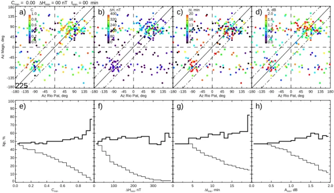
Cmin = 0.00 ∆Hmin = 00 nT tmin = 00 min
-180 -135 -90 -45 0 45 90 135
Az Rio Pat, deg -180 -135 -90 -45 0 45 90 135 180 Az Magn, deg a) 225 0.0 0.2 0.4 0.6 0.8 1.0 C -180 -135 -90 -45 0 45 90 135
Az Rio Pat, deg
b) 0 80 160 240 320 400 ∆H, nT -180 -135 -90 -45 0 45 90 135
Az Rio Pat, deg
c) 4 7 10 13 16 20 ∆t, min -180 -135 -90 -45 0 45 90 135 180
Az Rio Pat, deg
d) 0.0 0.4 0.8 1.2 1.6 2.0 A, dB 0.0 0.2 0.4 0.6 0.8 Cmin 0 10 20 30 40 50 60 70 80 90 100 Np, % e) 0 100 200 300 ∆Hmin, nT f) 0 5 10 15 ∆tmin, min g) 0.0 0.5 1.0 1.5 2.0 Amin, dB h)
Fig. 3. Scatter plots of the azimuth of the electrojet plasma flow versus the azimuth of the absorption patch drift. Each dot is colour coded in (a) correlation coefficient C, (b) total magnitude of horizontal perturbations 1H , (c) patch duration 1t, and (d) absorption intensity A. The colour code bar is shown in the top left corner of each panel. The total number of points is indicated in the bottom left corner of panel (a). Panels (e)–(h) show by a heavy black line the percentage of points above a certain threshold in parameter from a respective panel (a)–(d)
that is located within 45◦of the ideal coincidence line. The thin line shows the percentage of points within 45◦and above a certain threshold
with respect to the total number of points.
long-duration patches 09 and 11) are clearly associated with the changes in the flow direction polarity indicated in Fig. 2e by the vertical solid lines. In the next section we explore the relationship between the absorption drifts and electrojet flow using the data for all 10 events.
4 Absorption patch drifts and electrojet flow
In Fig. 3 we compare (point-by-point) the azimuth of the ab-sorption patch drift with the average azimuth (for the patch duration) of electrojet flow for all considered events, Table 1. Altogether 225 absorption patches were identified using the method described in Sect. 3. To identify the parameter(s) that might affect the quality of the absorption patch velocity determination, all points in Fig. 3 are colour-coded in (a) cor-relation coefficient C= min(Cx, Cy), (b) the total magnitude
of horizontal magnetic perturbations 1H , (c) patch duration 1t, and (d) absorption intensity maximum A. As mentioned, 1t was limited by 20 min. The maximum values for 1H and A were 850 nT and 5.3 dB, respectively, with the ma-jority (>∼90%) of points having 1H <400 nT, A<2 dB. In the correlation coefficient calculations we discarded one out-sider point to eliminate the effects of the sudden jumps (by less than 100 km) in the CNA maximum location with suc-cessive return to the original position that most likely did not represent the actual motion but rather a sudden, short-lived
(1–2 min) CNA intensification at some other location within the same patch, as, for example, at 04:46 UT in Figs. 1, 2c, 2d. One can see that, similar to the previous section, there is a general agreement between the azimuths; the majority of points are within 45◦ of the ideal coincidence line (we selected a ± 45◦limit simply as a boundary between direc-tions that are closer to the plasma drift direction and the ones that are closer to the perpendicular direction; these bound-aries are shown by dash-dotted lines). Of the four param-eters of interest, the points with greater C, 1t, and A tend to concentrate in the vicinity of the ideal coincidence line. To emphasize this point, we show in panels (e)–(h) with a heavy line the number of points above a certain threshold in the respective parameter with a relatively good agreement (±45◦ of the ideal coincidence) divided by the number of
all points above the same threshold (in %). For reference we also show with a thin line the percentage of points with good agreement with respect to the total number (225). Thus, for example, from panel (e), 50% of points with the correla-tion coefficient C between 0.5 and 1.0 have good agreement, while in total the points with C =0.5–1.0 and good agree-ment constitute 25% of all 225 points. Clearly, the agreeagree-ment improves with the increase in C, 1t , and A, while it does not change much with the 1H increase. We also notice that the percentage of points with larger 1H drops faster (thin line) than in any other histogram. Having that in mind, for further analysis we restricted the database of absorption patches by
Cmin = 0.50 ∆Hmin = 30 nT tmin = 10 min
-180 -135 -90 -45 0 45 90 135 180
Az Rio Pat, deg -180 -135 -90 -45 0 45 90 135 180 Az Magn, deg a) 46 -300 -200 -100 0 100 200 300 Vx, m/s -300 -200 -100 0 100 200 300 -∆ X, nT 0.0 0.4 0.8 1.2 1.6 2.0 A, dB b)
Fig. 4. Panel (a) The same as Fig. 3d but with additional criteria ap-plied. Panel (b) shows the scatter plot of the magnetic perturbations
−1Xversus zonal velocity of patch motion Vx.
imposing the following criteria: Cmin≡0.5, 1Hmin≡30 nT,
and 1tmin≡10 min.
Figure 4a shows the points that satisfy these new criteria. In total, there are 46 absorption patches in the new database. One can immediately notice that the agreement is indeed much better. The analysis analogous to that of Figs. 3e–h shows that at least 70% of points are within 45◦of the ideal coincidence line. The points with worst agreement tend to have smaller absorption maximum values. In panel (b) we show a similar scatter plot, the reversed north component of magnetic perturbations −1X versus zonal component of the patch drift velocity Vx. The sign of the magnetic
perturba-tions is opposite to that of the zonal component of drift ve-locity (except for 4 points in the bottom-right and top-left quadrants). The points of the same sign are all located close to zero, both in terms of velocity and magnetic perturbations. The points with small absorption tend to have small veloc-ities and magnetic perturbations. The zonal velocveloc-ities are not high, with the typical values of the order of 150 m/s for both east- and westward drifts. Magnetic perturbations, on the other hand, tend to be smaller in amplitude for westward propagating patches than for eastward drifting ones (50 nT versus 50–200 nT).
One can conclude from Figs. 3, 4 that the absorption patches drift in the direction which is close to that of the elec-trojet plasma flow derived from magnetic perturbations. If so, the absorption patches should reverse their drift direction (from eastward to westward) at the same time as the elec-trojet flow does. In the example presented in Fig. 2 we saw that this was approximately the case; from the keogram, the absorption drift reversal was observed at 07:22 UT, close to the reversal in magnetic azimuth at 07:16 UT (vertical solid line in Fig. 2e). The analysis of the absorption patch motion based on the tracing of the absorption maximum in succes-sive locations confirmed this result; patch 10 (∼07:00 UT) was drifting eastward, while patch 11 (∼07:15 UT) was drift-ing westward. To assess how well the reversals in the riome-ter and magnetomeriome-ter data correspond to each other in all 10 events we performed the following analysis.
The absorption drift direction reversals trev keowere
iden-tified from the keograms for all 10 events (two for event 2);
3 5 7 9 UT -40 -30 -20 -10 0 10 20 30 40 dT, min 2 2 3 4 5 6 7 8 9 10 a)
10
3 5 7 9 UT 2 2 3 4 5 6 7 8 8 9 10 b)11
Fig. 5. The time difference between the motion direction rever-sals as determined from two different methods versus the reversal time from the second method: (a) from the absorption images and keograms and (b) from the absorption images and magnetic pertur-bations. The total number of points is indicated in the bottom left corner of each panel. The diamonds mark the points that are farther from the zero time difference than the estimate uncertainty (verti-cal bars). The digits by each point indicate the event number from Table 1.
these reversals are given in the last column of Table 1. The drift reversals were also determined from the analysis of the drift direction for successive absorption patches as described below. We first identified successive patches with zonal drifts in opposite directions and above a threshold of 20◦in drift
az-imuth magnitude. Only the absorption patches of sufficiently long duration 1tmin=7 min and high correlation coefficient
(the highest of the two) Cmin=0.6 were considered here. The
absorption patch drift reversal time was then set to the mean of the start time of the first patch tst1 and the end time of the second patch tend2 , trev pat≡(tst1+tend2 )/2. The uncertainty in
reversal time in this method was set to (tend2 −tst1)/2. The re-versal time estimates calculated in this method were shown in Fig. 2e by the dotted vertical lines with the uncertainties shown by the dashed vertical lines.
To check that the two methods of reversal time calcu-lations (from the keograms and from the absorption im-ages) give comparable results we plotted the time difference trev keo−trev pat versus trev keo in Fig. 5a. The uncertainty
in trev keo was assumed to be zero for the present purpose.
Digits near each point indicate the event number from Ta-ble 1. There are 10 (out of 11 total) reversals trev keo that
have a corresponding reversal trev pat within 30 min. The
points are clustered evenly around the horizontal line of ideal coincidence and only one point (7, marked by the diamond) is farther from the zero line than the estimate uncertainty. In panel (b) we compare the reversal times from the mag-netometer data trev magn (shown by solid vertical lines in
Fig. 2e) with the closest reversals trev pat (dotted lines in
Fig. 2e) by plotting the difference between those against trev magn. Again, with the exception of event 1 all reversals in
the electrojet flow had corresponding reversals in absorption patch drift direction. Two reversals (both in magnetometer and riometer data) were identified for event 8, whereas only
-180 -135 -90 -45 0 45 90 135 180 Az, deg 00 01 02 03 04 05 06 07 08 09 10 11 12 13 14 15 16 1718
a)
04 05 06 07 08 09 Universal Time 0 250 500 750 1000 1250 1500 Vel Horiz, m/s IRIS EISCAT 00 0102 03 04 05 06 07 08 09 10 11 1213 14 15 16 17 18b)
Fig. 6. Comparison of the IRIS absorption drift and EISCAT convection velocities in (a) azimuth and (b) magnitude. Blue lines show the absorption drifts with the digits indicating the patch number from Fig. 2e. Diamonds connected with the thin lines correspond to the EISCAT ion drift measurements at 2-min resolution simultaneous with the absorption patches from Figs. 1, 2e (the colour scheme is the same as in Fig. 2e). Green horizontal lines show the average EISCAT ion drift velocities (for the patch duration).
one such reversal was identified in keogram. The overall agreement is satisfactory, with only two points located far-ther from the zero line than the estimate uncertainty. A sim-ilar result was obtained by plotting trev magn−trev keoversus trev keo (not presented here). One can conclude that within
the estimate uncertainty the reversals in the riometer absorp-tion drift direcabsorp-tion were almost coincident with the reversals in the electrojet flow direction derived from magnetic pertur-bations.
5 Ion drifts and ionospheric conductances from the EISCAT measurements
In the previous section we compared the absorption drift di-rections with those of the electrojet plasma flow derived from the magnetic perturbations under an assumption that the lat-ter are mainly produced by the Hall ionospheric currents and showed that these directions were close to each other. A com-parison of the absorption drifts and Doppler velocities mea-sured by ionospheric radars such as CUTLASS (HF), STARE (VHF), and EISCAT (UHF) is another way of exploring the relationship between the absorption drift and plasma convec-tion. Unfortunately, during none of the 10 events of interest the HF/VHF echo occurrence near the IRIS FoV was high enough to produce reliable convection velocity estimates.
The EISCAT tristatic ion drift velocity measurements from which the plasma convection velocity in the F-region (E×B drift) can be inferred, were performed only during one event (14 February 2001) and in this section we present these data. One should note, however, that the quality of the EISCAT data during this event was not fully conducive for compar-isons with the IRIS-inferred drifts, e.g. for the exact zonal drift reversal time determination, partly due to the technical problem with remote site computers (the transmitter power was not transmitted properly to the remote sites), resulting in minor measurement errors introduced during the data analy-sis for which a fixed value of the transmitter power had to be assumed.
In Fig. 6 we present the comparison between the IRIS and EISCAT horizontal velocities in (a) geographic azimuth and (b) magnitude for 14 February 2001, 04:00–09:00 UT. Blue lines represent the IRIS absorption patch drifts from Fig. 2e. The digits nearby show the patch number. Diamonds show the EISCAT horizontal velocities at 2-min resolution. The average EISCAT velocities (for the patch duration) are shown by green lines and the EISCAT data points used for this av-eraging (including points above the maximum velocity in panel (b)) are colour-coded according to the colour scheme of Fig. 2e. We have excluded all points with unrealistically high velocity VEI SCAT>5 km/s.
The EISCAT convection velocity gradually changes its di-rection from eastward to westward, panel (a), although the scatter in the EISCAT data points is quite large (except for the last 30 min). The reversal occurs between 06:30 and 08:00 UT. The agreement between IRIS and EISCAT drift di-rection is quite good, especially for patches with higher cor-relation coefficients 00, 04, 05, and 10 (shown as in Fig. 2e by thicker lines). Unfortunately, there is no simultaneous EISCAT data for the critical, westward drifting patch 15. The only “good” patch for which the difference in azimuths is above 15◦ is patch 03. We would like to point out, how-ever, that this large difference is almost entirely due to one blue point with negative azimuth of −135◦at ∼04:52 UT. The agreement between velocity magnitudes is much worse, panel (b), with the IRIS drifts being significantly lower, though one can notice that the EISCAT drifts decrease to-wards the middle of the interval of interest (06:00 UT), where the IRIS drifts are minimized as well (patch 07) and that for the intervals with smaller point scatter the disagreement is smaller, too. The latter suggests that the relatively large dis-agreement between velocity magnitudes could be related to the rapid fluctuations in the electric field intensity that are not seen through the imaging riometer technique but detected by incoherent radar as occasional high-velocity measurements, which, on average, result in larger EISCAT velocity magni-tudes.
Another issue that should be addressed in the context of the EISCAT data is the relationship between the absorption drift and ionospheric conductance. More specifically, we at-tempt to relate absorption to the height-integrated conduc-tivity and to assess the role that the conductance gradients may play in the determination of the Hall current direction from equivalent currents. Indeed, even though inferring this direction from the magnetometer records is rather a stan-dard technique (e.g. Stauning et al., 1995), its applicability may be questionable when, for example, the electron den-sity/conductivity distribution in the ionosphere is not homo-geneous as discussed below.
The height-integrated horizontal ionospheric current J is related to the Pedersen (6P) and Hall (6H) conductances
and electric field through Ohm’s law:
J = 6PE + 6H(ˆb × E) , (1)
where ˆb≡B/B is assumed to point downwards. The curl of the toroidal (divergence-free) component of the current JT
identical with the equivalent current Jeq derived from
mag-netic perturbations is given by:
∇ ×JT = ∇ ×(6PE) + ∇ × (6Hb × E)ˆ (2)
and can be approximated as:
∇ ×JT ∼= ∇6P ×E + ∇6H×(ˆb × E) + 6Hb∇ · E . (3)ˆ
To derive the real electrojet currents J from the mag-netic perturbations one needs the information on the large-scale distribution of either ionospheric conductances (e.g.
Kamide et al., 1981) or electric fields from which the for-mer can be estimated (Inhester et al., 1992; Amm, 1995). Since the imaging riometer data from which the conduc-tance gradients can be inferred, was available only near the KIL magnetometer site and since the electric field distribu-tion (e.g. from coherent radars) informadistribu-tion was not avail-able, we are not in a position to accurately compute the real currents. In addition, global techniques applied to the lo-cal problems often lead to large uncertainties (Murison et al., 1985; Knipp et al., 1994). We can nevertheless estimate the effects of the conductance gradients on the errors associated with the assumption that the equivalent currents are equal to the Hall currents/conductance homogeneity. Thus, from Eq. (3), this error depends on the relative contribution of the first term as compared to the other two terms and hence on the ratios ∇6P/∇6H and ∇6P/6H. Under the
assump-tion of the fixed ratio α≡6H/6P at any point, it follows that ∇6P/∇6H=1/α and ∇6P/6H=1/α∇6H/6H. Hence,
we should consider the relative gradient ∇6H/6H.
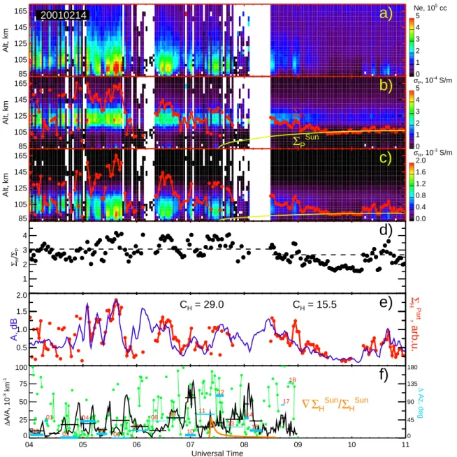
We next present the EISCAT data and ionospheric char-acteristics derived from these measurements and model pa-rameters. Figure 7a shows the EISCAT electron density data from 84.4 to 173.5 km on 14 February 2001, 04:00– 11:00 UT. The raw data from the Tromsø site have been analyzed with a 2-min resolution using the alternating cod-ing scheme. The minimal altitude of 84.4 km was selected, since during the analysis it was found that the density data below the fully decoded altitude of 87.4 km (90-km range) exhibited regular changes that were consistent with the den-sity measurements above 87.4 km in at least one 3-km gate. The EISCAT densities have been calibrated using the Tromsø Dynasonde data for the same period. The data points that had negative densities or temperatures (not shown) have been excluded from further analysis. Panels (b) and (c) show the Pedersen and Hall conductivities, respectively, estimated from the EISCAT densities, electron temperatures and model collision frequencies according to the standard formulas (e.g. Kelley, 1989, p. 39). The collision frequencies have been calculated by using the expressions given by Schunk and Walker (1973) and Schunk and Nagy (1978) and neutral at-mosphere density profiles given by the MSISE-90 thermo-spheric model for the time (14 February 2001, 06:00 and 09:00 UT, for night- and daytime measurements, respec-tively) and location of measurements (IRIS FoV centre). The red dots in panels (b) and (c) are the height-integrated (84– 173 km) Pedersen (6P) and Hall (6H) conductivities in
ar-bitrary scale. These values have been assigned to a spe-cific time only if the percentage of altitude ranges with den-sity/temperature data was above 50%, so that the intervals when the EISCAT measurements were patchy (as, for exam-ple, near 08:00 UT) have been excluded. Finally, the yellow curves show the model height-integrated conductivities due to the sunlight (Robinson and Vondrak, 1984). The ratio be-tween Hall and Pedersen conductances α, panel (d), was of the order of 3 for the entire period of interest. This ratio was slightly higher during the night.
85 105 125 145 165 Alt, km 0 1 2 3 4 5 Ne, 105 cc
a)
20010214 85 105 125 145 165 Alt, kmΣ
PΣ
P Sun 0 1 2 3 4 5 σP, 10 -4 S/mb)
85 105 125 145 165 Alt, km 0.0 0.4 0.8 1.2 1.6 2.0 σH, 10 -3 S/mc)
1 2 3 4 ΣH / ΣPd)
A, dB 0.5 1.0 1.5 2.0 Σ H Part , arb.u.e)
CH = 29.0 CH = 15.5 04 05 06 07 08 09 10 11 0 25 50 75 100 ∆ A/A, 10 -3 km -1 Universal Time ∆ Az, deg 0 45 90 135 180 00 01 03 04 05 06 07 08 09 10 11 12 13 14 15 17 18f)
Σ
H Sun/
Σ
H Sun∆
Fig. 7. Ionospheric conductances from the EISCAT measurements on 14 February 2001, 04:00–11:00 UT. First three panels show (a)
the electron density Ne, (b) Pedersen conductivity σP, and (c) Hall conductivity σH from 84.4 to 173.5 km. The colour bars are shown
on the right of each panel. Also shown in panels (b) and (c) by red dots and lines are the Pedersen (6P) and Hall (6H) conductances,
respectively, and the model conductances (6PSunand 6SunH ) due to the sunlight (Robinson and Vondrak, 1984). Panel (d) shows the ratio
α = 6H/6Pwith the average night- and daytime ratios (3.06 and 2.66, respectively) shown by dashed lines. Panel (e) shows the absorption
intensity at IRIS beam 16 (blue), together with the normalized Hall conductance due to the particle precipitation 6P artH (red). The scaling
coefficient CH = 6HP art/Ais different for night- and daytime conditions, as indicated on the top of panel (e). The red dots in panel (e)
are connected only if the difference between neighbour points is less than 0.5 dB. The bottom panel (f) shows by a black line the relative gradient of absorption 1A/A at the IRIS FoV centre (IRIS beam 25) and by blue lines the difference in drift azimuths 1Az= |Az Magn
−Az Rio| as determined from absorption images and magnetometer records from Fig. 2e. The relative gradient of the conductance due to
the sunlight ∇6SunH /6SunH is shown by the orange line. The black horizontal lines indicate the average relative absorption gradients (for the
patch duration). The instantaneous (1-min resolution) difference in azimuths is shown by green dots (connected if the difference between
neighbour points <45◦).
In panel (e) we show by blue line the absorption intensity measured in beam 16 of IRIS, the beam closest to that of EISCAT at 90 km. The Hall conductance due to the particle precipitation only, 6HP art≡
q
6H2 −(6HSun)2, is shown in
panel (e) by red dots/lines in arbitrary scale. The scaling coefficients CH=6HP art/Awere selected separately for the
night- and daytime conditions. Some of the red dots are significantly lower than the blue line, but more detailed inspection reveals that these points in most of the cases refer
-180 -135 -90 -45 0 45 90 135 Az Rio Pat, deg -180 -135 -90 -45 0 45 90 135 Az a, deg a) 00 03 04 05 06 07 15 07 -180 -135 -90 -45 0 45 90 135
Az Rio Pat, deg
Az b, deg b) 0003 04 05 06 07 15
Fig. 8. The azimuth of the patch’s (a) longest and (b) shortest di-mension versus azimuth of the patch drift from 14 February 2001
for Cmin=0.5, 1Hmin=30 nT, 1tmin=10 min. The digits by each
point indicate the patch number, Figs. 1, 2e.
to those 2-min intervals during which density is greatly reduced as compared to the intervals immediately before and after, as, for example, at 07:22 and 07:32 UT. In general, however, absorption A is correlated quite well with the Hall conductance due to the particle precipitation 6HP art.
Assuming that a similar relationship exists also for any other point within the IRIS FoV, the effects of the con-ductance gradients on the agreement between riometer- and magnetometer-inferred drift directions can be estimated. We have to remember, however, that consideration of the rela-tive gradients is more appropriate, as discussed above. Fig-ure 7f shows the comparison between the relative gradi-ent in absorption intensity 1A/A at the IRIS FoV cen-tre and the difference between drift directions determined from riometer (Az Rio) and magnetometer (Az Magn) data. The relative gradient in conductance due to the sunlight ∇6SunH /6SunH is shown by the orange line. The average dif-ferences 1Az≡|Az Rio–Az Magn| taken from Fig. 2e are shown by horizontal blue lines and the average relative ab-sorption gradients (for the patch duration) are shown by black lines.
The relative gradients due to the sunlight ∇6HSun/6HSun are small, except for the interval immediately af-ter the sunrise (07:22 UT) and even then they are smaller than the gradients associated with the parti-cle precipitation 1A/A∼=∇6HP art/6HP art. The depen-dence ∇6H 6H =F ( ∇6Sun H 6SunH , ∇6P art H
6HP art ) is rather complex because
of the nonlinear dependence of 6H upon 6HSun and 6HP art but from Fig. 7f it can be approximated as ∇6H/6H∼=∇6P artH /6HP art∼1A/A for almost the entire
period of interest. There is no clear relationship between the average 1Az and 1A/A, e.g. patches 03 and 04 are associ-ated with the comparable 1A/A (black) but 1Az (blue) is much larger for patch 04. One might think that a comparison of the average parameters is less meaningful in a situation when gradients at a fixed observational point exhibit high
variability, while the absorption drifts are estimated from the tracing of the absorption patches in the entire FoV and that a similar comparison on a smaller time scale could be more ap-propriate. To achieve this we computed the “instantaneous” differences in azimuths in a manner similar to that described in Sect. 3, except that instead of considering the motion of the absorption intensity maximum for long intervals (10–20 min) we considered the motions for each 1 min of measurements. To reduce the data scatter inevitable in such a crude method of velocity determination we discarded all 1-min intervals during which the absorption maximum jumped by more than 25 km. We show these instantaneous differences by green dots, Fig. 7f. Despite the difference in approach, one still cannot recognize any clear relationship between gradients and the difference in azimuths, except for the interval 05:00– 06:00 UT when the larger differences are associated with the larger gradients. Interestingly enough, this was also the in-terval during which the absorption was highly correlated with the Hall conductance, Fig. 7e.
6 Absorption patch drifts and orientation
In Fig. 1 we presented an example of the absorption inten-sity images that showed a large variability in the absorption patch shape, orientation, and drift velocity. In this section we further explore the relationship between the direction of absorption patch drift and those of the patch’s longest and shortest dimensions (determined as described in Sect. 3). In Fig. 8a (8b) we have plotted the azimuth of the patch’s longest (shortest) dimension, “Az a” (“Az b”), versus az-imuth of the patch drift direction, “Az Rio Pat”. As before, we limited the number of patches from 14 February 2001 us-ing criteria Cmin=0.5, 1Hmin=30 nT, 1tmin=10 min. The
digits near each point in Fig. 8 indicate the patch number. Figure 8 also shows the standard deviations for azimuth of the longest and shortest dimensions.
In case of the elongated region with enhanced absorption propagating in the direction perpendicular to the direction of elongation one would expect that the azimuths of the ab-sorption patch’s longest dimension (Az a) would be located near the lines that denote perpendicularity with the patch drift direction (outer diagonal lines), while the azimuths of the shortest dimension (Az b) would be located close to the ideal coincidence line (solid diagonal line). Figure 8 con-firms these expectations but only to a certain extent. Indeed, from Fig. 8b, the direction of the shortest dimension is very close to the drift direction. In Fig. 8a, however, quite a few points lie within ±45◦lines, that is closer to the drift vec-tor than to the perpendicular direction. The standard devia-tions for some points in both estimates, however, were quite large. To reduce uncertainties associated with these particu-lar estimates, for the next diagram we restricted the database to encompass only the points with standard deviations less than 30◦, Fig. 9. From the event on 14 February 2001 only points 04 and 06 have sufficiently small deviations, so that in this diagram we show the data from all events. In addition, to
σa max = 30 0
σb max = 30 0
-180 -135 -90 -45 0 45 90 135
Az Rio Pat, deg -180 -135 -90 -45 0 45 90 135 Az a, deg a) 17 0.0 0.4 0.8 1.2 1.6 2.0 A, dB -180 -135 -90 -45 0 45 90 135
Az Rio Pat, deg
Az b, deg
b)
Fig. 9. The same as Fig. 8 but for all events and patches when the standard deviation in average azimuth (both for longest and shortest
dimensions) was below 30◦. The points are colour-coded in
ab-sorption intensity. The colour bar is shown in the top left corner of panel (a).
check whether the absorption intensity has any effect on the data in this presentation, all points in Fig. 9 are colour coded in absorption. Despite the limitations, the situation is quite similar to that of Fig. 8. The majority of points in Fig. 9b are located close to the ideal coincidence line, whereas there are at least 4 points in Fig. 9a with sufficiently small deviations to say for sure that they are also located close to the drift di-rection. Finally, there seems to be no consistent pattern in Fig. 9 with respect to the absorption intensity.
7 Absorption patch drifts from images and keograms In Sect. 3 we described two methods of the absorption patch velocity calculations, the first method is based on the trac-ing of the absorption intensity maximum positions in the absorption “square-shaped” FoV images, deriving velocity components from the regression lines, and constructing the total drift velocity vector as a simple vectorial sum of com-ponents. An alternative way is to use the information from the single row and column of the riometer beams (“cross-shaped” FoV), which is the case, for example, for presen-tation in the form of absorption keograms. In this method, however, the construction of the total drift velocity vector is not so straightforward (see below) and in general requires making an assumption about the direction of the drift. More precisely, an arc-like absorption enhancement is often as-sumed to propagate perpendicular to the direction of elon-gation. The data presented in this report, on the other hand, suggest that this is not always the case (Figs. 1, 9a).
In Fig. 10 we illustrate the motion of an elongated patch and the patch velocity calculations, assuming an arbitrary patch drift direction with respect to the patch elongation. As the patch drifts from the initial position, shown by dark grey ellipse, to the final position (light grey ellipse), the successive narrow riometer beams along the x and y axes would record the passage of the absorption maximum through the beam,
q
d
V
dx
y
Vax VayV
d=
V /cos
ad
az
d= p/2-q+d
VaFig. 10. Motion of elongated absorption patch. The initial (final) patch position is shown by the dark (light) ellipse. The velocity of
apparent motion (perpendicular to the longest patch dimension) Va
is obtained from the apparent velocities along the axes Vaxand Vay.
from the timing of which the apparent velocities Vax and Vay, respectively, can be deduced. Using these values and
assuming a certain rotation of the drift velocity vector from the direction perpendicular to elongation (angle δ in Fig. 10) the total patch velocity can be constructed as follows: θ =tan−1Vax Vay , Va=Vaxcos θ , (4) azd = π 2 −θ + δ, Vd=Va/cos δ , (5)
where Vaand θ (Vdand azd) are the magnitude and direction
of the apparent (true) drift velocity vector. Note that the an-gle θ is counted from the x axis counterclockwise, while the drift azimuth azdis counted from the y axis in the clockwise
direction.
The second method (from the apparent motion in keograms) is limited in a sense that the angle δ has to be assumed, whereas the first method (from the absorption im-ages) can provide both the total velocity vector Vd and the
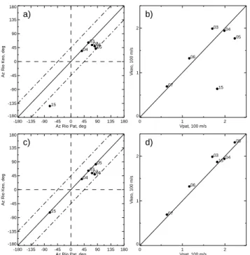
angle δ. It is, therefore, of particular interest to compare the drift velocities obtained using these two methods. Fig-ures 11a–b show the result of such a comparison for (a) drift azimuths and (b) drift magnitudes from 14 February 2001, assuming δ≡0. The digits by each point indicate the patch number (in the numeration scheme of Figs. 1 and 2e). The drift velocity from the absorption keograms (“Az Rio Keo” and Vkeo) was calculated for the closest (within 20 min)
“keogram patch” to those “image patches” that satisfied the criteria of Fig. 4. Thus, patches 03–07, 15 (Figs. 1, 2e) are compared with patches 00–04, 07 in Figs. 2a–b. The over-all agreement in Figs. 11a–b is satisfactory. The points 05 and 15 have the worst agreement, both in terms of azimuth and magnitude; for both patches the keogram method under-estimates the drift velocity. The reason for this underestima-tion can be the finite rotaunderestima-tion of the drift velocity vector away from the perpendicularity with the patch elongation. Accord-ing to Eq. (5), the drift velocity increases with δ as 1/ cos δ,
-180 -135 -90 -45 0 45 90 135 180 Az Rio Pat, deg
-180 -135 -90 -45 0 45 90 135 180
Az Rio Keo, deg
03 04 05 06 07 15 a) 0 1 2 Vpat, 100 m/s 0 1 2 Vkeo, 100 m/s 03 04 05 06 07 15 b) -180 -135 -90 -45 0 45 90 135 180
Az Rio Pat, deg -180 -135 -90 -45 0 45 90 135 180
Az Rio Keo, deg
03 04 05 06 07 15 c) 0 1 2 Vpat, 100 m/s 0 1 2 Vkeo, 100 m/s 03 04 05 06 07 15 d)
Fig. 11. Comparison of the (a) azimuths and (b) speeds of the patch drift motion on 14 February 2001 as determined from absorption keograms and images. The digits by each point indicate the patch number, Figs. 1, 2e. Panels (c) and (d) show the same comparison but with the assumed additional rotation of the velocity vector for points 05 and 15.
so that one can introduce a necessary correction for velocity simply by assuming some finite angle δ. Figures 11c–d show the same comparison as Figs. 11a–b, but with “correction” angles δ=40◦and δ=70◦for patches 05 and 15, respectively. One can see a significantly better agreement both in magni-tude and azimuth of the drift velocity. The correction angles are in agreement with the data presented in Fig. 8a, in which the average deviations from perpendicularity were 58◦ and
77◦for patches 05 and 15, respectively, with the uncertainties
of ∼40◦. Thus, using velocities of the patch apparent
mo-tion inferred from the keograms and by assuming that some patches were drifting in a direction that was different from perpendicularity to elongation, it is possible to reproduce the results obtained from the absorption images.
8 Summary and discussion
In this study we concentrated on the motions of the steadily drifting absorption structures in the morning sector. For the analysis we selected 10 events featuring the change in the zonal component of drift velocity from east- to westward.
In the past, zonally propagating absorption structures have been associated with the precipitating electrons injected into the nightside ionosphere at substorm expansion phase onset. The motion of electrons with energies in excess of 25 keV (required to produce a considerable absorption) is expected to be governed by the combined effect of the inhomogeneity
and curvature of the geomagnetic field (GC drift) (Roed-erer, 1967, 1970). Experimentally, however, Berkey et al. (1974) demonstrated that, even though in most events the observed velocities of the absorption eastward expansion of 0.7–7 km/s were close to velocities expected for the 50– 300 keV electrons, during some events the eastward expan-sion velocity was as high as 20 km/s, which would require unrealistically high energies if the GC drift interpretation was to be used.
In our observations, the absorption drifts were much slow-er, with the typical zonal velocities of the order of 150 m/s, Fig. 4b. For these velocities to be associated with the GC mechanism the precipitating electrons should be very soft (ε<10 keV) and hence very unlikely to cause a noticeable absorption on the ground. A similar result was obtained in the study by Hargreaves and Berry (1976), who reported the median absorption peak eastward speeds of 38 km/min (633 m/s). In an earlier study by Hargreaves (1970) the range of reported speeds was wider (from 80 m/s to 3.3 km/s), but for midnight observations the drift direction was pre-dominantly westward, in sharp contrast with the gradient-curvature hypothesis which implies eastward drifts for all time sectors. The great variability in velocity in Hargreaves (1970) suggested that the absorption structures move with the E×B rather than with the gradient-curvature drift. Later, Kikuchi and Yamagishi (1990) and Kikuchi et al. (1990) presented evidence that the drift pattern of the small-scale (30–60 km in width) absorption structures was essentially the same as the drift pattern derived by Hargreaves (1970) using riometers separated by ∼250 km. Kikuchi et al. (1990) also noticed a similarity between the absorption drift pattern and that of magnetospheric convection, although the data statis-tics was relatively low (13 drift events). In this context the absorption drift observations in various time sectors become of crucial importance. Kainuma et al. (2001) considered 106 absorption drift events between 13:00 and 07:00 MLT and found a reasonable agreement between their results and those of Hargreaves (1970) and Kikuchi et al. (1990).
In the present study we considered a comparable number of drift events (225 events without restrictions and 46 with re-strictions, Sect. 4) in the morning sector (06:00–12:00 MLT) the observations from which were poorly represented in the previous studies. The auroral absorption drift observations from these magnetic local times are also important, since one can expect the ionospheric convection to be reversed near magnetic noon, so that one can check whether the sense of absorption drift is reversed, too. Following this idea, instead of plotting the drift velocities for each individual drift event versus MLT in a statistical fashion similar to previous stud-ies (Hargreaves, 1970; Kikuchi et al., 1990; Kainuma et al., 2001), we considered a series of drift events, thus monitor-ing the absorption motions continuously, which allowed us to identify the reversal times. We would like to note here that the present report appears to be the first example of con-tinuous observations of absorption drifts that showed a clear change in the sense of zonal motions.