HAL Id: hal-00566971
https://hal.archives-ouvertes.fr/hal-00566971
Submitted on 17 Feb 2011
HAL is a multi-disciplinary open access archive for the deposit and dissemination of sci-entific research documents, whether they are pub-lished or not. The documents may come from teaching and research institutions in France or abroad, or from public or private research centers.
L’archive ouverte pluridisciplinaire HAL, est destinée au dépôt et à la diffusion de documents scientifiques de niveau recherche, publiés ou non, émanant des établissements d’enseignement et de recherche français ou étrangers, des laboratoires publics ou privés.
The Resilience of the Indian Economy to Rising Oil
Prices as a Validation Test for a Global
Energy-Environment-Economy CGE Model
Céline Guivarch, Stéphane Hallegatte, Renaud Crassous
To cite this version:
Céline Guivarch, Stéphane Hallegatte, Renaud Crassous. The Resilience of the Indian Economy to Rising Oil Prices as a Validation Test for a Global Energy-Environment-Economy CGE Model. Energy Policy, Elsevier, 2009, 37 (11), pp.4259-4266. �10.1016/j.enpol.2009.05.025�. �hal-00566971�
The Resilience of the Indian Economy to Rising Oil Prices as a Validation Test for a Global Energy-Environment-Economy CGE Model
Céline Guivarcha,* , Stéphane Hallegattea,b, Renaud Crassousa,c
a Centre International de Recherche sur l’Environnement et le Développement, Nogent-sur-Marne,
France
b Ecole Nationale de la Météorologie, Météo-France, Toulouse, France
c AgroParisTech – Institut , Paris, France
* Corresponding author at: CIRED, 45bis, Av. de la Belle Gabrielle, F-94736 Nogent-sur-Marne, France.
Tel.: +33 1 43 94 73 86; fax: +33 1 43 94 73 70. E-mail address: guivarch@centre-cired.fr (C. Guivarch).
Reference to this paper should be made as follows: Guivarch, C., Hallegatte, H., Crassous, R., 2009, ‘The resilience of the Indian economy to rising oil prices as a validation test for a global energy–environment–economy CGE model’, Energy Policy 37:11, 4259–4266.
Abstract
This paper proposes to test the global hybrid computable general equilibrium model
IMACLIM-R against macroeconomic data. To do so, it compares the modeled and
observed responses of the Indian economy to the rise of oil price during the
2003-2006 period. The objective is twofold: first, to disentangle the various mechanisms
and policies at play in India’s economy response to rising oil prices and, second, to
validate our model as a tool capable of reproducing short-run statistical data. With
default parameterization, the model predicts a significant decrease in the Indian
growth rate that is not observed. However, this discrepancy is corrected if three
additional mechanisms identified by the International Monetary Fund are introduced,
namely the rise in exports of refined oil products, the imbalance of the trade balance
allowed by large capital inflows, and the incomplete pass-through of the oil price
provides interesting insights on the modeling methodology relevant to represent an
economy’s response to a shock, as well as on how short-term mechanisms – and
policy action – can smooth the negative impacts of energy price shocks or climate
policies.
Running headline: Validation Test for a Global E3 CGE Model.
Keywords: Global CGE model, Oil shock, Model validation.
1. Introduction
In the five decades since Johansen’s model of Norway, computable general
equilibrium models (CGE) have become influential tools for both research and policy
analysis. In more recent years, the twin challenges of energy security and climate
change have driven intense modeling efforts, which led in particular to the
development of hybrid CGE models (e.g., Bataille et al., 2006, Bosetti et al., 2006,
Edenhofer et al., 2006, Schäfer and Jacoby, 2006). These models aim at providing a
consistent framework to represent the interactions between macroeconomic
mechanisms and the energy sector (Hourcade et al., 2006) and became widespread to
make long-term projections of energy-environment-economy (E3) scenarios. The
IMACLIM-R model (Sassi et al., 2007), developed in CIRED, counts among these
hybrid CGE models. It is a global model with 12 regions and 12 sectors, its
architecture is based on a recursive general equilibrium model with sectoral
technico-economic modules inserted. A detailed description of the model’s architecture is
As with any model, a key question is its validation and the determination of its
validity domain. It appears all the more important as some serious questions have
been raised about the empirical validity of CGE models (the econometric critique,
e.g. McKitrick, 1998). In particular they are criticized for relying on one year’s data
to project decades in the future and for not modeling observations (Barker, 2004 and
Scrieciu, 2007). The usual explanation for the discrepancy between CGE models
projections and observations is that these models are designed to explore long-term
issues (over decades) and do not represent short-term adjustments, whereas economic
data are largely driven by short-scale processes. We claim, however, that this
explanation is not satisfying: this article will show that testing a long-term model on
economic data perturbed by short-term mechanisms is possible and useful in the
sense that it can improve the credibility of the tools used for quantitative policy
advice.
In this article, the response of the Indian economy to the rapid oil prices rise of the
recent years will be investigated. India was chosen for this test because, in our
model, India is highly vulnerable to oil shocks. For instance, for default
parameterization of the model, India exhibits a 38% decrease in growth rate for an
81% increase in international oil price between 2003 and 2005, which is at odds with
the observed resilience of the Indian economy to rising oil price over this period.
Investigating why the modeled response of the Indian economy is not consistent with
current observations will, therefore, be particularly useful to assess our model and
give insights on the modeling methodology relevant to represent an economy’s
We analyze the response of the Indian economy over the 2003-2006 period, because,
over this period, economic data are available and no other large shock affected India.
Before 2003, the Indian economy is still heavily affected by the consequences of the
2001 crisis in the U.S. After this period, macroeconomic aggregate estimates are not
available yet.
In this paper, we have a twofold objective: on the one hand to disentangle the various
types of mechanisms at play in India’s economy response to rising oil prices and on
the other hand to validate IMACLIM-R as a tool capable of reproducing short-run
statistical data. Our methodology is the following. First, we compare the observed
response of the Indian economy to the increase in oil world price and the response
modeled with the standard calibration of our model. As shown in Section 2, there are
very significant differences between the observed and modeled responses. In
particular, the model predicts a much stronger decline in annual growth than what is
observed. Second, we explore, in Section 3, whether the assumptions on labor
productivity growth on which the model lies can be the source of this discrepancy, as
labor productivity growth is the major growth driver together with population
growth. We show that they cannot be the only explanation, except with implausibly
high labor productivity growth. Third, we study in Section 4 alternative explanations
for this discrepancy, from the February 2006 IMF country report on India
(Fernandez, 2006): (1) the large capital inflow in India; (2) the incomplete
pass-through of oil world price in the Indian market; (3) the rise of India as an exporter of
refined products. We then include these mechanisms by changing the
parameterization of the model and assess the ability of our modified model to
taking into account the three short-term mechanisms identified above modifies the
model results, and allows the model to reproduce fairly well the recently observed
response of India to rising oil prices. Section 6 concludes and proposes leads for
future research.
2. Modeling macroeconomic response to oil shocks: a first modeling test
Since the first oil shock in 1973, an abundant literature explored the relationship
between energy prices and growth, on both the empirical side and the theoretical
side1. On the empirical side, most of the analyses have focused on the U.S. and found
that oil price shocks have affected output and inflation. In particular, Hamilton
(1983, 1996) showed in a series of influential works that increases in the price of oil
were followed by periods of recession in the US. On the theoretical side,
considerable efforts were devoted to understand the nature and size of the
interactions between the oil price and macroeconomic aggregates. There appears to
be no consensus, and competing or complementary theories coexist2. Notably,
Bernanke (1983) indicates oil price shocks lower value added because firms
postpone their investments decisions while finding out whether the oil price increase
is temporary or permanent, whereas Bruno and Sachs (1985) propose the
“wage-price spiral” explanation: to prevent the real wage from falling, a decline in value
added is necessary in response to an oil shock. Olson (1988) shows a potential
channel of transmission is the transfer of wealth involved in paying higher oil import
bills, and Hamilton (1988) suggests the recession is due to a shift in demand causing
the decrease in output following oil price increase involves oligopolistic behaviours
of firms, whereas Finn (2000) imputes this decrease to variable capital utilization of
firms under perfect competition. Bernanke, Gertler and Watson (1997) focus on the
recessive effect of monetary tightening in response to the inflation risk.
The previous paragraph highlighted the theoretical complexity of the interactions
between oil prices and macroeconomic aggregates. Our interest in this paper is
focused on how large-scale models can draw on this complexity and represent the
response to an oil price shock, which appears particularly difficult. On the one hand,
Jones et al. (2004) assert that macro-models (IMF’s MULTIMOD, OECD’s
INTERLINK, FRB’s FRB/Global) are structurally unable to reproduce the
magnitude of the economic response to oil price shock, as they resort to single-sector
production functions and therefore do not capture the intersectoral resource (labor,
capital, materials) reallocation costs. On the other hand, E3 CGE models represent
intersectoral interactions but Barker (2004) affirms that they are unsuited to model
adjustment to price changes such as responses to oil price shocks because they are
concerned with a set of equilibrium positions and do not represent transitional
adjustment paths. Their limit, indeed, is to rest on modeling choices (full utilization
of production factors, maximizing representative agents under perfect foresight,
flexible production functions) that, most of the time, lead to instantaneous and
frictionless readjustment to a new optimal growth path after perturbations. As a
consequence, E3 CGE models represent long-term bifurcations but cannot capture
IMACLIM-R architecture was developed to try and overcome the two shortcomings
aforementioned (Crassous et al., 2006a, 2006b and Sassi et al., 2007). It is a hybrid
model in two senses. (1) It is a hybrid model in the classical sense: its structure is
designed to combine Bottom-Up information in a Top-Down consistent
macroeconomic framework. Energy is explicitly represented in both money metric
values and physical quantities so as to capture the specific role of energy sectors and
their interaction with the rest of the economy. The existence of explicit physical
variables allows indeed a rigorous incorporation of sector based information about
how final demand and technical systems are transformed by economic incentives. (2)
It is hybrid in the sense of Solow (2000)3, i.e. it tries and bridge the gap between
long-run and short-run macroeconomics, as efforts were devoted not only to model
long-term mechanisms but also focus on transition and disequilibrium pathways. We
seek, indeed, to capture the transition costs with a modeling architecture that allows
for endogenous disequilibrium generated by the inertia in adapting to new economic
conditions due to both imperfect foresight and non flexible characteristics of
equipment vintages available at each period (putty-clay technologies). The inertia
inhibits an automatic and costless return to steady-state equilibrium after an
exogenous shock. In the short run the main available flexibility lies in the rate of
utilization of capacities, which may induce excess or shortage of production factors,
unemployment and unequal profitability of capital across sectors.
Our model is calibrated on 2001 data from GTAP 5 database (Dimaranan and
McDougall, 2002). Default parametrization comprise (i) exogenous trends for
demography (UN World Population Prospects, medium scenario, UN, 2004) and for
article), (ii) resorption of international capital flows on the long term, (iii)
Armington’s specification (Armington, 1969) for non-energy goods trade and a
standard market-share equation depending on relative export prices for energy goods
trade (so as to be able to sum physical quantities and track consistent energy
balances).
To test our modeling architecture, we perform a first run of the model (simulation 1),
with default assumptions for all exogenous parameters (in the following, referred to
as the original version of the model). This model is exactly the one used for
long-term scenarios development, but run over the 2003-2006 period only. In this
simulation, the oil price is fixed exogenously, to follow the observed oil price
between 2001 and 2007 (see left panel of Fig. 1). The right panel of this figure shows
the Indian GDP growth in this simulation. With a rising oil price, the modeled GDP
growth decrease from 7.6% in 2003 to about 6.3% in 2004 and between 4.8% and
5.4% in 2005 and 2006, whereas, with constant oil prices (simulation 2), growth
remains between 9% and 8% over this period. This figure shows clearly that, in the
model, the Indian economy is highly vulnerable to variations of the international oil
price. The model reveals an oil price-GDP elasticity equal to -0.048, a median value
compared to estimates summarized in Jones et al. (2004) ranging from -0.02 to -0.11.
But this result is at odds with recent observations in India: according to the World
Bank, the Indian GDP growth lied between 8 and 10% during this period, showing
the robustness of the Indian economy. The model, therefore, does not reproduce
In the following, we will pursuit a twofold objective: first to try and explain why
India's resilience to the rise of oil prices is not reproduced by our model; and second,
to demonstrate whether our model results can approach observations, provided that
additional mechanisms are included in the analysis. We will show that this exercise
gives interesting insights on both the various mechanisms and policies at play in an
economy’s response to a shock and the modeling methodology appropriate to
represent this response.
3. Labor productivity gains as an explanation for India’s resilience to the rise of oil prices?
Our model growth engine is composed of exogenous demographic trends and
technical progress that increases labor productivity, as in Solow’s neoclassical model
of economic growth (Solow, 1956). Demography simply follows UN scenarios but
technical progress entails more uncertainty on the short-run. Solow’s model (Solow,
1957) and following developments on growth accounting make technical change the
residual of growth unexplained by demography or capital accumulation. Endogenous
growth theories (see for instance Aghion and Howitt, 1992) explore the mechanisms
at play behind technical change but the theoretical and empirical researches in this
field are far too complex to be directly applied in models for long-term projections in
the climate and energy domain. This is why we use exogenous trends of productivity
growth, as it is a common practice in the energy-environment modeling community.
To build these trends we draw on stylized facts from the literature, in particular the
on economic convergence, one investigating the past trends by Maddison (1995), and
the other one looking at future trends, by Oliveira Martins (2005). For India, default
assumptions for labor productivity growth lie between 5.7% and 5.3% over the
2003-2006 period (Fig. 2).
The two sets of assumptions on demography and technical change, although
exogenous, only prescribe potential growth. Effective growth results endogenously
from the interaction of these driving forces with short-term constraints: (i) available
capital flows for investments and (ii) not full utilization of production factors (labor
and capital) due to the inadequacy between flexible relative prices (including wages)
and inert capital vintages characteristics.
As a consequence, the difference between our model’s results and observations may
arise from the growth engine or from the short-term constraints. We first try and
reproduce the observed growth rate by modifying the growth engine. The
demographic scenarios we use are adjusted on the short-term to follow actual
demography statistics. Therefore, the uncertainty on the growth engine, over the
short-term period we consider, lies mainly in the assumptions on technical change.
Figure 2 shows the mean labor productivity growth assumptions that are necessary to
make the model reproduce observed GDP growth (simulation 3). In these
assumptions, labor productivity growth reaches a peak at 14% in 2005.
These assumptions seem too high to be acceptable, in particular if checked against
the limited set of data available on labor productivity in India (Bosworth and Collins,
respectively on the period 1993-2004. We may also cite as an upper bound for
plausible assumptions the labor productivity growth observed during economic
take-off in Europe or Japan in the postwar period or in the Asian “dragons” (e.g. a peak at
9% in France in 19694, and 8.7% in South Korea in 19835). Furthermore it seems
unrealistic that the peak in labor productivity growth takes place precisely the year
when oil price growth is the highest, as labor productivity growth results in fact from
economic activity dynamics.
As it is difficult to obtain reliable data on sectoral labor productivity growth, it is
impossible to calibrate our model with real data on this point, but we may consider
the original assumptions on labor productivity growth as more reasonable. In the
following, we will therefore look for other mechanisms likely to explain the
difference between the observed and modeled responses to the oil price rise, without
resorting to accelerating the model growth engine.
4. In search for other mechanisms
The robustness of the Indian economy has been recently analyzed in a section of the
February 2006 IMF country report on India (Fernandez, 2006). The report identifies
four key mechanisms that explain the strong Indian growth despite rising oil prices:
(1) The sectoral reallocation of resources (away from oil-intensive activities) has
been able to take place smoothly as the economy experiences rapid
(2) Large foreign currency reserves and strong capital inflows have limited the
economy's need to adjust;
(3) The incomplete pass-through of international petroleum prices has
moderated the income effect on domestic consumers;
(4) The rise of India as an exporter of refined products has moderated the impact
of the terms of trade shock and the transfer of income abroad.
The first mechanism, referring to the structural change towards a lower importance
of oil intensive activities and a greater importance of the service sector, is already
present in our model. It is taken into account by the internal response of the model,
which reproduces the sector interactions within the economic system. Figure 3 shows
sectors contributions to the growth of added value, in the model results and
according to World Bank data. It reveals that the model represents fairly well the
sectoral structural change towards a greater importance of the service sector, which
contributes to around 60% of the growth of total added value in both the model
results and statistical data. The evolution of the TPES/GDP indicator, reduced by
3.2% over the 2003-2006 period in the model’s results and by 3.9% according to EIA
data, also confirms that the model reproduces the aggregate effect of efficiency gains
and structural change.
The last three mechanisms, on the opposite, are not taken into account by the model.
First, as it is common practice in our field (e.g. Edmonds et al., 2004, Paltsev et al.,
2005), the default assumption concerning capital flows in the model is that the trade
balance and capital flows tend to zero over time in all countries, and that price levels
difficulty in predicting capital market and exchange rate dynamics, as country
attractiveness for investments ensues from many complex factors including political
stability and corruption risk, and many others. Second, we assume in the original
version of the model that the tax and subvention structure and the government budget
structure are not modified in response to the rise in oil price. This assumption is
made necessary by the high difficulty to predict, and all the more to model, the
political response to an exogenous shock. These two shortcomings are acceptable in
a long-term model because these imbalances can exist over the short-term but are not
sustainable over the long-term: a government cannot increase its deficit or the
country trade deficit for ever to compensate for increasing oil prices. Third, the
endogenous formation of prices and export shares in the model does not reproduce
the magnitude of the rise in Indian refined products exports: modeled export value of
refined oil products evolves from 2.1 billion dollars in 2003 to 3.1 in 2006, whereas
statistics show a rise to 6.1 billion dollars in 2006. This is due to the fact that the
coefficients of the market-share equation representing energy goods trade are
calibrated on 2001 data when India’s exports of refined products represented a very
small share of all traded refined products.
Since the model is tested against data that obviously include these mechanisms, these
additional mechanisms need to be taken into account by the model in this validation
exercise. In the following, we will exogenously introduce these mechanisms in our
modeling exercises.
To see if the model is able to reproduce the observation, the three missing explaining
factors identified in the previous section have been introduced in the model. It is out
of the scope of this paper to model the full complexity of these mechanisms. To take
them into account, therefore, we modified the parameterization of some elements in
the model so as to approximate the aforementioned mechanisms.
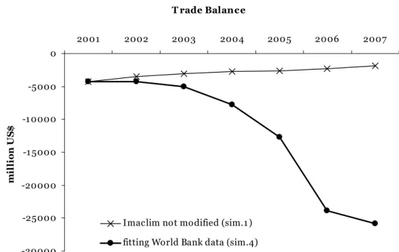
First, to model the effect of the strong capital inflows into India and the large foreign
currency reserves of this country, we forced the imports of capital into India, from all
other countries, so that the Indian trade balance6 fits to the statistical data (simulation
4), whereas in the initial version of the model the country imports of capital remain a
constant share of all international capital flows (see Figure 4).
Second, to represent the incomplete pass-through of international petroleum prices to
domestic consumers, we introduced a government subsidy to oil products
consumption that takes the form of tax reductions (simulation 5). Alternatively, we
could have chosen to channel the subsidy through cuts in the government-owned
petroleum company margins, which would have given similar results as more than
95% of petroleum products consumed are domestically refined. The resulting fiscal
deficit is financed by a fraction of the foreign capital inflow, which can be seen as an
increase of the government foreign debt (even if debt mechanisms are not explicitly
modeled in the current version of the model). According to data from the IMF
country report, we represent a 40% pass-through, i.e. the fact that domestic oil price
Finally, the rise of India as an exporter of refined products is reproduced by forcing
exogenously the volume of refined-product exports to follow the data (simulation 6),
while the original model calculates it endogenously from the interplay between
supply, demand and relative prices.
Figure 5 shows the results of the initial model (simulation 1) and of several model
versions, including one7 (simulations 4, 5 and 6), or all of these three additional
short-term mechanisms (simulation 7). It shows that, while the original model
simulates a strong decline in GDP growth, the modified model version that includes
the three additional mechanisms is close to observations. Our results, therefore,
confirm that the three aforementioned mechanisms are able to explain why the Indian
GDP growth remained at a high level in the 2003-2006 period despite rising oil
prices.
Adding the three factors one by one allows one to discriminate their respective
contribution in narrowing the gap between the model initial results and the data. In
our model at least, the dominating effect is the disequilibrium of the trade balance
that is permitted by strong capital inflows. This mechanism alone increases GDP
growth by more than 2% in 2005. As a comparison, the partial pass-through alone is
only able to increase growth by less than 1%, and the rise in exports can hardly be
distinguished from the baseline produced by the original model.
The simulation in which the three mechanisms are included gives growth rates
relatively close to statistical data. Indeed, for 2005, the year for which the difference
9.2%. These results show how short-term flexibility, here through changes in trade
balance and capital flows in particular, can influence in a significant manner
short-term GDP growth, and smooth exogenous shocks.
As an additional test of our modified model version, we compare in Figure 6, the
evolution of the sectors shares in added value given by the model and observed.
These results show that the model does not only reproduce aggregate growth, but is
also able to capture fairly well its sectoral distribution8.
Finally, we show that the model’s results in terms of oil import and refined products
consumption fit broadly with available data: over the 2003-2006 period, the mean
annual increase of oil import volumes is 5.3% in simulation 7 results against 7.0% in
ENERDATA data, and the mean annual increase of refined products consumptions is
3.0% in modeling results against 3.9% in data. It appears that the model
underestimate slightly oil imports and refined products consumption, but it might be
linked to the GDP growth that remains slightly lower in simulation 7 than observed
growth.
Of course, our results are not perfect and there is still a difference between our model
results and the observed response of the Indian economy. Section 2 showed that
changes in productivity growth alone could not explain the resilience of the Indian
economy. They may, however, explain the small remaining difference between the
modeled and observed economy. We may now look for the appropriate labor
productivity growth assumptions (simulation 8) that should be introduced in the
(Fig. 7). They appear to remain in a plausible interval, as they peak at 8%. We may
note that results from this simulation 8 concerning oil import and consumption are
now slightly above data: 7.6% mean annual increase of oil import volumes over
2003-2006 (7.0% in data) and 6.2% mean annual increase of oil products
consumption (3.9% in data). In terms of oil import and consumption, simulation 7
and simulation 8 bound data.
We may also suggest that the GDP growth difference between our simulation 7 and
the observations is partly due to other economic mechanisms that are imperfectly
reproduced by our model, such as the response of the informal economy, or the
response of the monetary policy, as explored notably in Blanchard and Gali (2007).
These mechanisms are important and require additional research to be included in a
global energy-economy model.
6. Conclusion
This paper is a first step toward a validation of our long-term global
energy-environment-economy CGE model against macroeconomic data. In its original
version, indeed, the model is not able to reproduce the observed Indian GDP growth
rate, and it overestimates the consequence of a rise in oil price on the economy.
Taking into account three mechanisms identified in the IMF country report and
disregarded in the original model modifies significantly the model results, and allows
the model to reproduce fairly well the observed economic data. In particular, these
in current models. Our results also have policy implications as they highlight two
mechanisms that smooth the adverse effect of oil shocks over the short term, and on
which the policy makers have partial control (the subsidy to oil products
consumption and the capital inflow or trade balance deficit). Moreover, the
respective effect of both mechanisms is assessed9, indicating that the most powerful
lever lies in the disequilibrium of the trade balance that is permitted by strong capital
inflows.
In terms of model validation, this paper remains partial, since it considers only a
single country, in a single period, and a single type of shock. It is needed, therefore,
to conduct similar tests for other countries or regions and other periods to further
assess our model; and with other models to discriminate among the various modeling
choices that are made in our research community.
From a methodological point of view, our results suggest that the inability of the
model to reproduce historical data arise from short-term mechanisms that are
explicitly disregarded. It appears, additionally, that the mechanisms that are needed
to reproduce the observed Indian response to the rise in oil price are bound to remain
short-term or local mechanisms. It seems unrealistic, indeed, that the trade balance
deficits keep growing for decades in all world energy-importing countries. Also,
government subsidies cannot keep offsetting price increases on the long run.
Therefore, it appears acceptable not to embark these mechanisms in our modeling
architecture when analyzing long-term and global evolutions. But these short-term
mechanisms might, however, play a major role in the transition dynamics, either to
case – or to amplify negative impacts if a short-term process acts as an amplifying
feedback. This is of particular importance for our modeling work. Indeed, following
the intuition that climate change mitigation costs are mainly transition costs,
IMACLIM-R architecture was specifically designed to explore transition pathways.
Important efforts were expended to represent the inertia (e.g., technical and
infrastructure inertia) responsible for transition costs and to model trajectories year
by year. But this paper indicates further efforts should be devoted now to explore
how short-term mechanisms, such as the temporary deficit of the trade balance, may
play a role in the transition to a low-carbon economy and allow to smooth adverse
effects of shocks.
Additionally, disregarding short-term mechanisms means assuming a complete
separation between short-term and long-term dynamics. This assumption is at the
heart of the growth theory but has been questioned by several authors (e.g., Solow,
1988; Arrow, 1989). We may thus conclude on another prospect for future research.
It is necessary to investigate how short-term mechanisms might influence long-term
growth pathways (see an attempt to do so in Hallegatte et al., 2008) or, in other
words, if there is a path-dependency of long-run growth. If this influence is
non-negligible, indeed, the analysis of short-run mechanisms will have an undeniable
place in the understanding of long-run macroeconomy, and modeling teams will have
to devote more time to the apprehension of the links between short-term dynamics
and long-term trajectories.
The authors wish to thank Olivier Sassi, Jean-Charles Hourcade and Philippe Quirion
for their useful comments and suggestions, as well as Henri Waisman, Meriem
Hamdi-Cherif, Sandrine Mathy and all the team who contributed to IMACLIM-R
development. We are also grateful to an anonymous reviewer who helped us improve
our article. This research was supported by the Chair 'Modeling for sustainable
development', led by MINES ParisTech, Ecole des Ponts ParisTech,
AgroParisTech and ParisTech, and financed by ADEME, EDF, RENAULT,
SCHNEIDER ELECTRIC and TOTAL. The views expressed in this article are the
authors’ and do not necessarily reflect the views of the aforementioned institutions.
References
Aghion, P., Howitt, P., 1992. Endogenous Growth Theory. MIT Press, Cambridge.
Armington, P. S., 1969. A Theory of demand for products distinguished by place of
production. IMF, International Monetary Fund Staff Papers 16, 170-201.
Arrow, K., 1989. Workshop on the economy as an evolving complex system:
summary. In: Anderson, P., Arrow, K., Pines, D. (Eds.), The Economy as an
Evolving Complex System. Addison-Wesley, New York, pp. 275–282.
Barker, T., 2004. The transition to sustainability: a comparison of General–
Paper, vol. 62. Tyndall Centre for Climate Change Research, University of East
Anglia, Norwich.
Barro, R. J., Sala-i-Martin, X., 1992. Convergence. Journal of Political Economy
100:2, 223-251.
Barsky, R.B., Kilian, L., 2004. Oil and the Macroeconomy since the 1970s. Journal
of Economic Perspectives 18:4, 115-134.
Bataille, C., Jaccard, M., Nyboer, J. and Rivers, N., 2006. Towards general
equilibrium in a technology-rich model with empirically estimated behavioral
parameters. The Energy Journal, Special Issue 2.
Bernanke, B.S., 1983. Irreversibility, uncertainty, and cyclical investment. Quarterly
Jounral of Economics 98:1, 85-106.
Bernanke, B.S., Gertler, M., and Watson, M.W., 1997. Systematic monetary policy
and the effects of oil price shocks. Brookings Papers on Economic Activity 1,
91-148.
Blanchard, O.J., Gali, J., 2007. The Macroeconomic effects of oil price shocks: Why
are the 2000s so different from the 1970s? International Dimensions of Monetary
Bosetti, Valentina, Carlo Carraro, Marzio Galeotti, Emanuele Massetti, and Massimo
Tavoni. (2006). WITCH: A World Induced Technical Change Hybrid model. The
Energy Journal, Special Issue 2.
Bosworth, B., Collins, S.M., 2007. Accounting for growth: Comparing China and
India. NBER Working Paper 12943.
Bruno, M., and Sachs, J.D., 1985. Economics of worldwide stagflation. Cambridge,
Harvard University Press.
Crassous, R., Hourcade, J.-C., Sassi, O., 2006a. Endogenous structural change and
climate targets: modeling experiments with Imaclim-R. Energy Journal, Special Issue
on the Innovation Modeling Comparison Project.
Crassous, R., Hourcade, J.-C., Sassi, O., Gitz, V., Mathy, S., Hamdi-Cherif, M.,
2006b. IMACLIM-R: a modeling framework for sustainable development issues.
Background paper for Dancing with Giants: China, India, and the Global Economy.
Institute for Policy Studies and the World Bank, Washington, DC. Available at
http://siteresources.worldbank.org/INTCHIINDGLOECO/Resources/IMACLIM-R_description.pdf.
Dimaranan, B.V., McDougall, R.A., 2002. Global Trade, Assistance, and Production:
Edenhofer, O., Lessmann, K., Bauer, N., 2006. Mitigation strategies and costs of
climate protection: The Effects of ETC in the hybrid model MIND. Energy Journal,
Special Issue on Endogenous Technological Change and the Economics of
Atmospheric Stabilisation.
Edmonds, J., Pitcher, H., Sands, R., 2004. Second General Model 2004: An
Overview. Available at http://www.globalchange.umd.edu/models/sgm/.
Finn, M.G., 2000. Perfect competition and the effects of energy price increases on
economic activity. Journal of Money, Credit and Banking 32:3, 400-416.
Hallegatte, S., Ghil, M., Dumas, P., Hourcade, J.-C., 2008. Business cycles,
bifurcations and chaos in a neo-classical model with investment dynamics. Journal of
Economic Behavior & Organization 67, 57–77.
Hamilton, J., 1983. Oil and the Macroeconomy since World War II. Journal of
Political Economy 91:2, 228-248.
Hamilton, J., 1988. A neoclassical model of unemployment and the business cycle.
Journal of Political Economy 96:3, 593-617.
Hamilton, J., 1996. This is what happened to the oil price macroeconomy
Hourcade, J.-C., Jaccard, M., Bataille, C., Ghersi, F., 2006. Hybrid modeling: New
answers to old challenges. The Energy Journal, Special Issue 2, 1-11.
Fernandez, E., 2006. Dealing with higher oil price in India. In: International
Monetary Fund, 2006. India: Selected Issues. IMF country Report 06/56.
Jones, D.W., Leiby, P.N., 1996. The Macroeconomic impacts of oil price shocks: A
Review of literature and issues. Oak Ridge National Laboratory.
Jones, D.W., Leiby, P.N., Paik, I.K., 2004. Oil price shocks and the macroeconomy:
What has been learned since 1996. The Energy Journal 25:2.
Maddison, A., 1995. Monitoring the world economy: 1820 – 1992. OECD
Development Center.
McKitrick, R., 1998. The econometric critique of computable general equilibrium
modelling: the role of functional forms. Economic Modelling 15:4, 543–573.
Oliveira Martins, J., Gonand, F., Antolin, P., de la Maisonneuve, C., Kwang, Y.,
2005. The impact of ageing on demand, factor markets and growth. OECD
Economics Department Working Papers 420.
Olson, M., 1988. The productivity slowdown, the oil shocks and the real cycle.
Paltsev, S., Reilly, J.M., Jacoby, H.D., Eckaus, R.S., McFarland, J., Sarofim, M.,
Asadoorian, M., Babiker, M., 2005. The MIT Emissions Prediction and Policy
Analysis (EPPA) Model: Version 4. MIT Joint Program Report 125. Available at:
http://web.mit.edu/globalchange/www/eppa.html.
Rotemberg, J., Woodford, M., 1996. Imperfect competition and the effects of energy
price increases on economic activity. Journal of Money, Credit and Banking 28:4,
549-577.
Sassi O., Crassous, R., Hourcade, J.-C., Gitz, V., Waisman H., Guivarch, C., 2007.
Imaclim-R: a modelling framework to simulate sustainable development pathways.
International Journal of Global Environmental Issues (accepted).
Schäfer, A., and Jacoby, H.D., 2006. Experiments with a Hybrid CGE-MARKAL
Model. The Energy Journal, Special Issue 2.
Scrieciu, S., 2007. The inherent dangers of using computable general equilibrium
models as a single integrated modelling framework for sustainability impact
assessment. A critical note on Böhringer and Löschel (2006). Ecological Economics
60, 678-684.
Solow, R., 1956. A Contribution to the Theory of Economic Growth. Quarterly
Solow, R., 1957. Technical change and the aggregate production function. Review of
Economics and Statistics 39, 312-320.
Solow, R., 2000. Toward a macroeconomics of the medium run. Journal of
Economic Perspectives 14:1, 151-158.
Figure 1
International oil price
0 1 0 20 30 40 5 0 60 7 0 80 2001 2002 2003 2004 2005 2006 2007 U S $ /b b l 0% 5% 1 0% 1 5% 20% 25 % 30% 35 % 40%
Oil price (US$/bbl) WRI data
oil price growth annual (%) (right ax is)
GDP growt h 0% 1 % 2 % 3 % 4 % 5% 6 % 7 % 8% 9 % 1 0% 2 003 2 004 2 005 2 006
World Bank data
Im aclim sim ulation with increasing oil prices (sim .1 ) Im aclim sim ulation with constant oil prices (sim .2 )
Figure 2
Labor productiv ity growth assum ptions
0% 2% 4% 6% 8% 1 0% 1 2% 1 4% 1 6% 2003 2004 2005 2006
modified growth engine (sim.3) original growth engine (sim.1 )
Figure 3
Sectors contribu tions to Added Value growth (m ean v alue 2003-2006) 0% 1 0% 20% 30% 40% 50% 60% 7 0%
A griculture Industry Serv ices
Imaclim-R simulation (sim.1 ) World Bank data
∆AVsector
Figure 4 T rade Balance -30000 -25000 -20000 -1 5000 -1 0000 -5000 0 2001 2002 2003 2004 2005 2006 2007 m il li o n U S $
Imaclim not modified (sim.1 ) fitting World Bank data (sim.4)
Figure 5 GDP growth 0% 2% 4% 6% 8% 1 0% 1 2% 2003 2004 2005 2006
Imaclim simulation not modified (sim.1 )
Imaclim simulation Trade Balance forced (sim.4) Imaclim simulation passthrough 40% (sim.5)
Imaclim simulation Ex porter refined products (sim.6) Imaclim simulation all three mechanisms added (sim.7 ) World Bank data
Figure 6
Sectors shares in Added Value in 2003
0% 1 0% 20% 30% 40% 50% 60%
Agriculture Industry Serv ices Imaclim-R simulation (sim.7 )
World Bank data
Annu al growth of sectors shares in added v alu e (mean v alue on 2003-2006) -20% -1 5% -1 0% -5% 0% 5% 1 0%
A griculture Industry Serv ices
Imaclim-R simulation (sim.7 ) World Bank data
Figure 7
Labor produ ctiv ity growth assu m ptions
0% 2% 4% 6% 8% 1 0% 1 2% 1 4% 1 6% 2003 2004 2005 2006
growth engine to fit data with the original v ersion of Imaclim-R (sim.3)
growth engine to fit data with the modified v ersion of Imaclim-R (sim.8)
Captions to Illustrations
Figure 1: Left panel: International oil price observed during the 2001-2007 period.
Right panel: GDP growth computed by the model for simulation 1 with increasing oil
prices (crosses) or simulation 2 with constant oil prices (triangles) or, and observed
by the World Bank (points).
Figure 2: Mean labor productivity growth assumptions, for the original model
(simulation 1) (grey dots) and for the modified (black triangles) growth engine, such
that the model reproduces observed GDP over the 2003-2006 period (simulation 3).
Figure 3: Sectors contribution to Added Value growth the 2003-2006 period, as
modeled (results from simulation 1) and in the World Bank data10.
Figure 4: Indian trade balance between 2001 and 2007, as modeled by the original
version of the model (crosses) and as observed by the World Bank (points). In the
modified model version, the trade balance is forced to follow the observations
(simulation 4).
Figure 5: Observed GDP growth in India between 2003 and 2006, and results of the
initial model version (simulation 1) and of several modified model versions,
including one (simulations 4, 5 and 6) or all additional short-term mechanisms
Figure 6: Sectors shares in Added Value in 2003 and their mean annual growth rate
over the 2003-2006 period, as modeled (results from simulation 7) and in the World
Bank data10.
Figure 7: Mean labor productivity growth assumptions to fit GDP data with the
original version of the model (simulation 3) (black triangles) and with the modified
1 See for example Jones and Leiby (1996) and Jones et al. (2004) for a detailed review of the literature.
2
See for instance Barsky and Kilian (2004) for a review of the various channels through which oil prices may operate that were put forward.
3
Solow (2000) : ‘I can easily imagine that there is a « true » macrodynamics, valid at every time scale. But it is fearfully complicated [...] At the five-to-ten-year time scale, we have to piece things together as best we can, and look for a hybrid model that will do the job.’
4 Source: INSEE. www.insee.fr. 5
Source: OECD.Stat. http://stats.oecd.org/wbos/Index.aspx.
6 Terminology and its link with the model’s representation should be clarified here: the balance of payments is the sum of the current account, the capital account and the financial account. The current account is composed of the trade balance, the net factor income from abroad (interest and dividends) and net unilateral transfers from abroad (such as foreign aid). The capital account is the sum of the foreign direct investment, portfolio investment (stocks and bonds) and other investments (for instance in currencies). The financial account is composed of transaction involving financial assets and liabilities between residents and non-residents. In our modelling architecture, (1) the financial account and investments other than foreign direct investment are not represented and (2) the net factor income from abroad, the net unilateral transfers from abroad and foreign direct investments are not
represented separately but grouped into what we may call (abusively) the “capital balance”. Therefore, the equilibrium of the balance of payment implies is in our model the equality of the absolute values of the trade balance and our “capital balance.” That is why forcing the capital inflow can be directly translated into a forcing of the trade balance in our model.
7
As we know that these mechanisms are not independent (e.g., the relatively lower oil price due to the subsidies is likely to have attracted more capital, influencing the capital inflow), simulations with only one mechanism are somehow artificial, but they are helpful to assess the relative importance of each of mechanism.
8
The additional mechanisms included in the model influence aggregate growth, but do not change in a significant manner the sectoral distribution of growth.
10 Part of the differences between modeled and observed sectors share lies in the fact the sectoral aggregation used in IMACLIM-R differ from the aggregation used in the World Bank database. For instance, food-processing industries are included in the agricultural sector in IMACLIM-R whereas it is counted in the industrial sector in the World Bank database.