3-D Geostatistical Seismic Inversion With Well Log Constraints

WELL LOG CONSTRAINTS

Jonathan Kane, William Rodi, and M. Nafi Toksoz

Earth Resources Laboratory

Department of Earth, Atmospheric, and Planetary Sciences

Massachusetts Institute of Technology

Cambridge, MA 02139

ABSTRACT

Information about reservoir properties usually comes from two sources: seismic data and well logs. The former provide an indirect, low resolution image of rock velocity and density. The latter provide direct, high resolution (but laterally sparse) sampling of these and other rock parameters. An important problem in reservoir characterization is how best to combine these data sets, allowing the well information to constrain the seismic inversion and, conversely, using the seismic data to spatially interpolate and extrapolate the well logs.

We develop a seismic/well log inversion method that combines geostatistical tech-niques for well log interpolation (Le., kriging) with a Monte Carlo search method for seismic inversion. We cast our inversion procedure in the form of a Bayesian maximum

a posteriori (MAP) estimation in which the prior is iteratively modified so that the algorithm converges to the model that maximizes the likelihood function.

We follow the approach used by Haas and Dubrule (1994) in their sequential in-version algorithm. Kriging is applied to the well data to obtain velocity estimates and their covariances for use as a priori constraints in the seismic inversion. Inversion of a complete 3-D seismic section is performed one trace at a time. The velocity profiles de-rived from previous seismic traces are incorporated as "pseudo well logs" in subsequent applications of kriging. Our version of this algorithm employs a more efficient Monte Carlo search method in the seismic inversion, and moves sequentially away from the wells so as to minimize the kriging variance at eachstep away from the inverted wells.

Numerical experiments with synthetic data demonstrate the viability of Our seis-mic/well data inversion scheme. Inversion is then performed on a real 3-D data set provided by Texaco.

Kane et ale

INTRODUCTION

The most accurate method for obtaining information about the subsurface properties of the Earth is to drill a hole, extract the rocks, and/or use well logging tools to sample petrophysical properties therein. This, unfortunately, is too expensive and difficult to do in more than a few sparse, isolated locations. To obtain the values of a petrophysical property over a larger three-dimensional domain requires the accurate extrapolation of known values as well as the use of indirect information supplied by remote sensing techniques.

This situation is germane to the petroleum industry, which seeks to infer the location of hydrocarbons given sparse well log data and indirect seismic data. The density and compressional wave velocity of seismic waves can be sampled at a small scale in the well logs and at a large scale, indirectly, with seismic waves. Results of decades of research have been applied to inferring the velocity and density of the Earth from seismic data. Since the 1980's this research has been applied to three dimensional exploration. Standard techniques for performing this inference are illustrated in several sources, including Yilmaz (1987). Typically, these methods seek only to locate singularities in the subsurface parameters, i.e., locations at which the petrophysical parameter fields are nondifferentiable (such as jump discontinuities or thin beds). Migration is a technique which takes seismic data and "migrates" the singularities back to their point of origin, either in time (time migration) or depth (depth migration). A summary of migration techniques can be found in Gardner (1985). Therefore, it is standard practice not to infer the actual values of the parameter of interest, but rather to generate images of the geometry of subsurface structures through migration. We will refer to standard methods of obtaining images of subsurface structures as "imaging," and call the actual estimation of the petrophysical parameter values "inversion." In this paper, we attempt to provide a methodology for taking seismic data that have been time migrated along with a few well logs and perform inversion for acoustic velocity. Although density is also a relevant parameter in seismic wave propagation, we assume it constant for computational reasons.

We first give a brief overview of random field theory. This provides a framework for describing a field of petrophysical parameters in probabilistic fashion. We then use this framework to pose the inverse problem of inferring a wave velocity field given sets of data related to it by an operator. Inversion is performed on a synthetic 2-D data set and then on a synthetic 3-D data set. This allows for an assessment of the performance of the inversion method. Finally, we demonstrate the inversion method on a real 3-D data set provided by Texaco.

STOCHASTIC DESCRIPTION OF GEOLOGY

Let us denote a parameter field of interest asv(x), wherevis defined over a spatial field

V which can contain either a finite, countably infinite, or uncountably infinite set of locations x. A description of a random field requires a multivariate probability density

p(.) to be defined over v(x). The parameter value at each spatial location is then a random variable (RV) and has its own marginal probability density function as well as a (possibly infinite) number of joint moments with the RVs at other spatial locations.

We will make certain assumptions which simplify analysis and the usage of random fields. First, we assume that the RVs are jointly Gaussian. Then, the joint probability distribution has the following form:

( ( )) _ exp[-Mv(x;) - /Lv(x;))TCv(Xi,Xj)-l(v(Xi) - /Lv(xill]

pvx - N I

(21r)2ICv

l'

where N:= number of elements in v.

From this we see that a Gaussian field is fully described by its bivariate moments (covariances) and its mean. The covariance of such a field is defined as:

(1) where

/LXi

=

E[V(Xi)]'

The function

CO

is known as the covariance function and describes the covariance between every two points in the region V. It is also known as the (auto-)covariogram, or, if normalized to have a maximum of 1, the (auto-)correlogram. We assume that

/LXi

=

0 for simplification.

A second assumption that simplifies the description of a random field is to assume that the random field of interest is stationary. Roughly, this implies that the statistics of the random field do not change with spatial location. The covariance function then takes a simple form that depends only on spatial separation, not spatial location:

S=Xi-Xj'

The distance it takes for this function to go from its maximum to almost 0 is known as the range or correlation length. This covariance function can take a number of forms. Two common ones are Gaussian and exponential. These functions have the following forms, respectively,

Kane et al.

where a is the correlation length and 0'2 is the variance at 0 separation. We use the

Gaussian covariance function exclusively.

An alternate, but equivalent, representation of the covariance function exists called the (semi-)variogram, or structure function, 2')'(s). The relationship between the

vari-ogram and the covariance function in the case of a zero-mean, stationary random field is:

2')'(s) = 2(C(O) - C(s)).

We show that the variogram exists for certain random fields for which the covariance function does not (nonstationary processes that have stationary increments). An exam-ple of such a process is Brownian motion, which has the following power law variogram:

2')'(s)

=

asP

o::;

f3 <

2.

A third, and necessary, simplifying assumption is to discretize the parameter field over the regionD. This allows numerical manipulation and estimation to be performed on a computer. The covariance structure of a discrete, countably finite Gaussian field can be put into a table that lists the covariance between each two RVs in the field. This table is known as the covariance matrix. Ifv is real then C is automatically symmetric. The assumption of stationarity causes the covariance matrix to have a Toepplitz form,

i.e., it has constant diagonals.

Thus, we are limiting ourselves to a countably finite number of parameters in D.

This final simplification inherently assumes that our discretization of the continuous field is sufficient to capture all relevant details.

Generating Realizations From Random Fields

Covariance functions lend themselves to generating realizations of random fields, which is required by the Monte Carlo inversion method used in this paper. This requires the generation of a random vector v(x) such that it has the prescribed C(s). Assuming a zero mean field, the following line of reasoning demonstrates how to generate the desired

v(x). We henceforth writev(Xi) as y for brevity and useyT to denote its transpose.

A computationally efficient method for generating realizations makes use of the Fourier transform. Denote the Fourier transform of a finite dimensional vector as F. We find that for a symmetric, positive definite matrix C we have the following relationship: C

=

FAFT where A is the spectrum of the covariance function. A has the useful property that it is a diagonal matrix with

VA

=

VAT. This allows us to do the following decomposition:

E[yyT]

=

F

AFT

=

FVA

VAFT

= FVAIVAFT

=

FVAE[wwT]VAFT

This tells us that v =

FVA

w. Thus we are filtering white noise to obtain a realization of our random field. We use this method throughout the paper.

BAYESIAN INVERSION

We present standard results of Bayesian inversion. For derivation and rigor see Tarantola

(1987). Inversion theory seeks to infer the value of a vector, v EV, given only a data vector y E Y, a noise vector n E N, and a mapping, H(V) H

y.

We call the set of elements v E V the model space and the elements y E Y the data space. Mapping

H(V) H Y can be noninvertible (no existence of an inverse) or not uniquely invertible (the existence of many inverses for a given data vector y). Also, the inverse mapping

H-1_{(Y) may not be a continuous mapping even ifH (V)is. This amounts to the problem}

that slight perturbations in y lead to large perturbations in H-1(y).

Each element of a vector v, n, or y is itself an element in another vector space. This is the vector space of finite variance random variables. The addition of this structure uponV,

N,

andY makes v, n, and y random vectors and allows us to perform Bayesian inversion.

To illustrate Bayesian inversion, we use a simple example Common to many fields of science. The problem is that of extrapolation. Extrapolation can be posed in the following way: Let vector v represent an element of the model space and mapping HK be a subset of the rows of the identity matrix, I. The operator selects which model parameters are observed and (possibly) adds some noise to them to give us the observed data y. v and n are random Gaussian vectors with associated covariance matrices, Cv

and Cn·

We write the forward problem as:

Matrix HK will be an P x Q matrix, where P is the number of observed elements y, and Q is the dimension of v. Thus, we have P

<

Q and are faced with the prob-lem of nonuniqueness. There are many models that fit the data, i.e., there are many interpolations that go through the data points but are different elsewhere.

Rearranging, we have:

n(v, y)

=

y - HKV.

We call this the noise function over the joint model and data space. Sometimes this is called the errorfunction, but we will reserve the word error for the norm of the misfit function, that is,

e(v,y)

=

Iln(v,y)IIP

for some 1 ::;p. For a given y

=

Yobs, we seek as our estimate:

v

=

mmE(e(v,y

=

Yobs)).

Kane et al.

Standard results give us the following expressions for the estimate "iT and its covari-ance matrix:

- C C-1

v= vy y Y

where Cvy is the cross-covariance between v and y. InEarth science these equations are

known as the kriging system of equations and are used to extrapolate sparse well data to unknown locations. C v and C" are often called the priorand posteriorcovariances, respectively.

For cases in which H is a nonlinear operator, inversion becomes more difficult. The optimal answer depends on which norm is used to define the error. The mini-mization procedure is more difficult because the error function is no longer quadratic and may have more than one inflection point. The goal remains to find the minimum of

E(e(v,y

=

Yobs)) but"iTis no longer a linearfunction ofy. Thus, a procedure is required that iterates over either the inverse or forward operator in order to minimizeE(e(v,y)). In the following sections, we use a Monte Carlo method for nonlinear estimation. Nonlinear Seismic Operator

The seismic forward modeling operator used in this paper, denoted Hs(')' is the most simple operator possible. It is known as the convolutional model. It assumes vertical incidence of plane seismic waves, no conversion to S-waves, no multiple scattering, and no loss of amplitude in the seismic signal as it travels through the medium. In order for this model to hold, the geology must be horizontally stratified and the raw seismic data time migrated. This processing produces a seismic trace at each vertical location of the model that is a function only of the acoustic velocity and density at that vertical location. We make a further simplification by assuming that the density is constant, which greatly reduces the computational complexity and allows us to invert for only one parameter.

HsO consists of three operations. First, an operation converts the vertical velocity field as a function of depth into velocity as a function of two-way traveltime:

v(z) t-+ vl(t).

Vi is then resampled onto a regular time series. The next operation produces the

reflec-tivity series:

r(t) =

~~lnv'(t) ~

v'(t+Ot) -v'(t).

2dt v'(t+Ot) +v'(t)

Finally, r(t) is convolved with known seismic wavelet, w(t), to produce the seismogram:

For a derivation of this operator see Sengbush et al. (1960). We write the relation between seismograms and velocity as

s = Hs(v)

+

n.

Although the dimension of s may be greater than v, there is no unique inverse to this operator. There are an infinite number of velocity vectors that all result in the same seismogram. To verify this, simply multiplyVi(t) by a constant and the resulting

seismogram does not change.

In the next section, we address how to find an inverse to the seismic operator and how to constrain it to choose one velocity vector from the infinite that fit the data.

Monte Carlo Inversion

In recent years, adaptive search methods have gained popularity as a tool for finding optimal solutions to geophysical inverse problems. Their popularity has been motivated by vast increases in computing power and the fact that these methods are more effective than traditional gradient-based methods in finding globally, rather than just locally, optimal solutions to nonlinear problems. Recent applications of adaptive search methods to seismic inversion include genetic algorithms (Sen et al., 1991), simulated annealing (Rothman, 1985; Stoffa and Sen, 1991; Vestergaard and Mosegaard, 1991), and iterative improvement (Haas and Dubrule, 1994).

The Monte Carlo method for estimating a solution to an inverse problem differs greatly from the linearized inverse methods presented above. The Monte Carlo method poses the inverse problem as an integration:

v

=

t

Iv

e(s

=

Sob"v)dv

where

e(s= Sob"v) = IIsob' - Hs(v) liP

V :=region of. integration.

HsO is the convolutional seismic operator from the previous section and Sob' is the

observed seismic data. Depending on the norm used to define the error function, a different solution will be obtained in the integration. Thep = 1 norm gives the median of posterior distribution, thep

=

2 norm gives the mean, and the p

=

00 norm leads to

a MAP solution. Furthermore, if the integrand can be split into two functions, we can obtain the same solution by sampling from one function and evaluating the other. This situation applies to Bayesian inversion where the posterior distribution can be split into

Kane et al.

a prior and a likelihood function. Itis usually easier to sample from the prior than the posterior!.

The Monte Carlo method approximates the above integral by a summation over the number of samples. It can be shown that, as the number of samples goes to 00, the

sample estimate approaches the solution

v.

The search algorithm employed by Haas and Dubrule (1994) is a simple Monte Carlo method, whereby the velocity estimate2_,

_v,

_{obtained from a given seismic trace, S, is a}

realization of a specified random process. Many realizations of the process are generated and the one yielding the maximum correlation is chosen as the solution. This is an easier criterion to fit than minimizing error. We will call Haas and Dubrule's method iterative improvement. The prior distribution that they use to generate velocity realizations is

the posterior mean and covariance resulting from kriging well data.

Our Monte Carlo search algorithm differs in two respects. First, we are minimizing error, not maximizing correlation. Second, we borrow a useful concept from simulated annealing: We allow the process from which realizations are generated to change adap-tively during the search. In simulated annealing, this is accomplished by specifying a temperature schedule, whose choice is one of the most difficult aspects of the algorith-m. Our approach is to gradually shift the mean and reduce the variance of the prior such that, like simulated annealing, the search becomes more and more local as better solutions are found. The "annealing" in our algorithm is not controlled by a tempera-ture schedule, but is determined only by the total number of trials. Our algorithm is basically a MAP estimation with a prior that progressively moves toward the minimum error model. This makes it a maximum likelihood estimator.

Proposed Monte Carlo Method

Our new Monte Carlo inversion method is easy to apply and provides good results for the convolutional seismic problem. The crux of this method is based on some properties of the following vector

v

=

ar+fJz,

where r and z are independent Gaussian vectors. The covariance matrix, Cv , of v can

therefore be expressed as

Ifwe further impose the constraint that

Cv

=

Cr

=

Cz

=

C,

---;-=----:-:---.,---...,.,---,-IThere are methods to sample directly from the posterior. Foremost among them is the Metropolis sample rejection method, which, in the case of posterior distribution estimation, leads to Gibbs sampling and in the case of maximum likelihood estimation leads to simulated annealing.

2Actually, Haas and Dubrule (1994) use acoustic impedance, but this equals velocity in our case of

the constants '" and fJ must satisfy

We therefore have three zero mean Gaussian random vectors, v, r, z, with the same covariance matrix. Below, we clarify the purpose of constructing v in such a way.

The algorithm proceeds as follows:

1. Perform kriging at a vertical location adjacent to a well log using well data within a specified distance of the kriged location. This gives a kriged mean vector, Ji-y for the pseudo well log and a kriged covariance matrix, Cy , which is approximately

stationary as a function of depth. This can be written as:

v

=

/-Lv

+

v*.

2. Specify the total number of iterations Ntot to be performed.

3. Fori = 1 ...N_{tot ,} let

where

Zi

=

Fy'Awi

and

or

4. As the algorithm proceeds, let

and fJ2 = - .i - I

Ntot

Thus, more and more weight will be applied to r while still ensuring that all realizations of v* have covariance Cy •

Kane et

al.

KRIGING AND SEISMIC INVERSION ON SYNTHETIC DATA

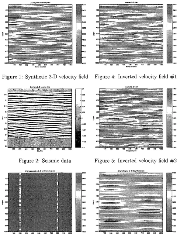
In this section, we apply the above inverse methods to synthetic data sets, first in 2-D and then in 3-D. A 2-D realization of a Gaussian random field is generated by the Fourier method. This field will be used to represent acoustic wave velocity. The input stochastic parameters needed to generate this field are the covariance function and the mean. C(s) in this case is an anisotropic Gaussian function with a horizontal correlation length ax = 200 ft and a vertical correlation length, _az = 10 ft. The variance of this field is ,,2

=

250,000 ft2/s2 and the mean is f.t

=

5000 ft/s. The realization is shown

in Figure 1. In performing all synthetic inversion, we assume we know the stochastic parameters a priori.

A 2-D seismic data set is generated from the velocity field using the

HsO

operator discussed above (see Figure 2). For inversion purposes we have, a priori, the seismic

wavelet used to create the synthetic seismic data. Estimating this wavelet in reality is a difficult task (see below).

Two wells are also extracted from this data set and, along with the seismic data, are used to do the inversion. The synthetic wells are shown in Figure 3. In this case, we can test the efficiency of the inversion process because we have the true model to compare it to after inverting the data.

We want to make optimal use of all the data in performing the inversion. Since each seismogram is dependent only on the velocity field at the same vertical location, we can sequentially invert one seismogram at a time. The first question is: "In what order should it be done?" The intuitively logical answer is to start inverting seismograms near the location of existing wells and proceed outward. Ifthere is any horizontal similarity in the velocity field (which we know a priori there is) then this procedure will make

inversion easier by constraining the inversion method to look for solutions similar to adjacent well data. This brings us to the second question: "How do we make use of the well data that we have?" The answer is to extrapolate the data with kriging. Kriging provides both an estimated mean and covariance at a vertical location. From these post-kriging stochastic parameters we can generate "pseudo" well logs. We use the Fourier method to generate these simulations. Normally, the post-kriging random field is quite nonstationary but in the special case of extrapolating vertical well logs to other vertical locations, the post-kriging field is approximately stationary. By way of generating these simulations, we employ our Monte Carlo method to search for the maximum likelihood model. When the best model is found it is included as more well data for the purpose of kriging further locations.

Some important differences should be pointed out between the method in Haas and Dubrule (1994) and the one presented here. They limit their parameter space to 30 samples in the vertical direction corresponding to a total of 120 ms. This corresponds to a few wiggles of their seismic trace, thus making it easier to fit the data. In contrast, the models used in our synthetic inversion are sampled in depth at 10 ft intervals for 1000 ft of depth and our seismic data consist of 256 samples at 0.002 ms discretization. Thus,

we have 100 parameters to invert for. Also, their algorithm performs sequential inversion by leap frogging horizontally through field locations. Haas and Dubrule perfonn the leap frogging because it helps give horizontal continuity to the inverted field. But, by doing the kriging at locations far away from the well data, the kriging variance is much higher. Thus, since there are an infinite number of models that fit the seismic data, there is a greater chance of converging to a suboptimal one. We, in contrast, perfonn the kriging at locations adjacent to well data. This minimizes the kriging variance and helps better constrain the inversion algorithm.

The 2-D field is inverted twice to show the variability of the inversion results. These two inversions are shown in Figures 4 and 5. Note how similar they are As a matter of fact, they look more like each other than the true field. It is unclear whv this is so, however, they all reproduce the main features of the true field, and' can be compared with the kriging results shown in Figure 6. We can see that performing kriging without conditioning it to the seismic data fails to reproduce the interwell variability.

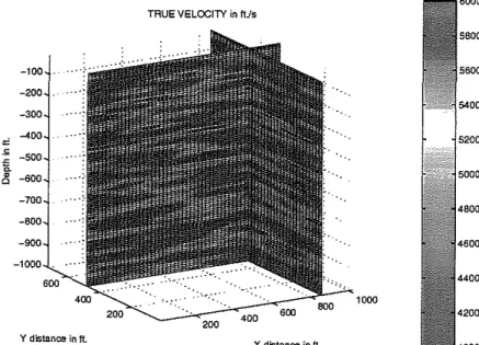
We now turn to 3-D inversion. Again, a Gaussian synthetic velocity field is created (Figure 7). It has identical stochastic parameters to the 2-D field with the inclusion of another horizontal correlation length a y

=

200 ft. A 3-D seismic data cube is also

produced from this model (not shown). We again use an a priori seismic wavelet in the

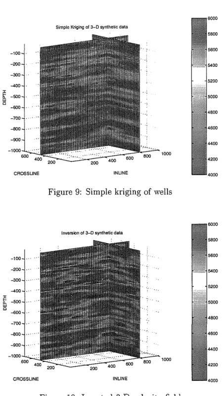
inversion. Five well logs are extracted from this field and are shown in Figure 8. Using these wells we first perform simple kriging in Figure 9. Some of the main features of the field are reproduced close to the wells but not beyond about a correlation length. We next perform sequential inversion on the same wells and seismic data. The results are shown in Figure 10, where we see great improvement over the kriging results.

There are 1836 seismic traces in the synthetic 3-D model and we perform 1000 Monte Carlo simulations for each trace. One entire 3-D inversion takes approximately four hours to complete. There are only 51 traces in the 2-D inversion, and again 1000 simulations are performed per trace. This takes only approximately seven minutes to run. All runs were performed on a 400 MHz Pentium 2 PC.

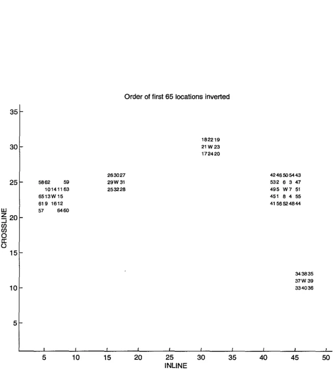
We should point out how the sequential algorithm moves from one vertical location to another. For 3-D inversion, the marching order is shown in Figure 11. This figure is a map view of the first 65 locations visited. Thus the inversion algorithm "propagates" out from each true well location. The same method is used for the 2-D model. Note also which data are included each time a location is kriged. It would seem logical to include all true well logs and previously inverted "pseudo" logs every time kriging is perfonned. This, however, gave poor results and increased computational time by an order of magnitude. Much better results were obtained when only the closest pseudo logs and a few far pseudo logs were included in the kriging. The farther ones are included just to help ensure continuity of the inverted field. At present, we cannot explain wh'l

this method is superior.

Kane et aI.

APPLICATION TO TEXACO DATA SET

The Texaco data set consists of five velocity well logs in a 3-D field (Figure 12). These logs were sampled at 0.5 ft intervals in depth. The seismic data consist of 1836 traces each sampled at 0.002IllSfor a total of 121 samples. Thus, 242IllSof data are recorded

at each trace. The well logs are truncated so that only the portion corresponding to 242 ms of time is included in the inversion. The average velocity in the well logs is 15,075

ft/s. This leads to approximately 3000 parameters to krig and invert at each pseudo

log location. This is far too computationally expensive for kriging and inversion, and may not be warranted ifthe well logs are significantly smooth at small scales. Unfor-tunately, the Texaco logs, like most logs, exhibit great variability even at the smallest scales. Despite this fact, we chose to smooth the logs in order to reduce the number of parameters. The velocity logs are smoothed enough to allow three decimations, that is, the sampling interval becomes 4 ft instead of 0.5 ft; we are left with"" 400 parameters to deal with in each log.

For the synthetic model used in the first inversion experiment, we knew a priori the covariance function describing the random field. This, however, is not the case for the Texaco data set. We attempt to estimate a variogram function for the velocity field in the vertical direction from available well logs. The variogram fit is shown in Figure 13. Itis fit with a Gaussian model with a vertical correlation length az

=

12 ft.

There is no satisfactory way to estimate the horizontal correlation lengths. Haas and Dubrule (1994) estimate them from the seismic data. From our experience, we find that the horizontal correlation lengths do not affect the inversion as long as they are chosen large enough to include immediately neighboring locations. Therefore, seeing that the seismic data are significantly correlated horizontally, we simply choose the horizontal correlation lengths to be 20 times the vertical length: ax

=

240ft, ay

=

240 ft. The variance of the velocity field is also obtained from the variogram and is 1,750,000ft2_/s2_•

We use all these parameters in the kriging and inversion of the Texaco data.

The main difficulty in working with real seismic data is that we need to extract a seismic wavelet. This is needed for theH

_s

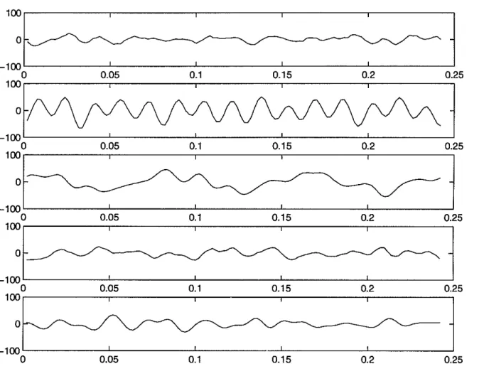
operator in the Monte Carlo search method. To extract a wavelet we need a seismogram and reflectivity series at the same place. We perform deconvolution on these two series to obtain the seismic wavelet. This was done at eachof the well log locations of the Texaco data with unsatisfactory results. Five different wavelets were extracted that looked significantly different from each other (see Figure 14). They also were not temporally limited the way one would expect a seismic wave to be. This problem illustrates the limitation of the convolutional model and questions its applicability. To perform sequential inversion, we can have only one wavelet, thus for lack of a better method, the wavelets were averaged and the resulting wavelet was used in the inversion.

We follow the same extrapolation pattern illustrated in Figure 11 with the Texaco data. Also, we allow 1000 Monte Carlo iterations at each pseudo log location that is inverted, just as was done for synthetic inversion. This number of iterations is again

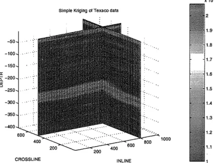
adequate to fit the seismic data even though the number of parameters being inverted for has increased four times. The results of the Texaco data set inversion are shown in Figure 16, and can be compared with the kriged results in Figure 15. The inversion brings out somewhat more detail but both have trends that persist horizontally through the field. Note that the figures show only the first 400 ft of the inverted model out of

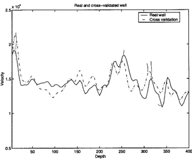
3000 ft. Matlab could not plot the entire model, hence only a sub volume is shown. We cannot check the accuracy of this inversion because we do not have the true field for comparison as we did with the synthetic -models. However, we can perform a

cross-validation by performing the entire inversion again without one of the true well

logs and comparing the results of the inversion at the location of the true well log. The results of the cross-validation at the true log location are shown in Figures 17 and 18 (again, only the first 400ft). We show the reflectivity because this is what the inversion is sensitive to. Remember the nonuniqueness-an infinite number of velocity models all have the same reflectivity series. While the velocities fit each other reasonably well, the reflectivity fits even better.

We can explain our good results by the fact that the seismograms only change slightly with horizontal distance. This implies that the underlying field is quite laterally continuous. Therefore, it seems easier for the inversion method to estimate the Texaco model than the synthetic model.

Note, finally, that the entire 3-D inversion of the TexacO- data required six hours of computing time.

CONCLUSIONS

We presented a method for inverting post-stack seismic data given limited well log data. Numerous methods exist to estimate petrophysical properties away from wells. Many methods also exISt to invert seismic data. However, few researchers have attempted to combine these methodologies in a coherent way. The results obtained show that sequentially extrapolating wells and inverting seismograms result in an accurate illver-sion of an unknown velocity field. The sequential extrapolation constrains the inverillver-sion with existing well data and the Monte Carlo algorithm handles the nonlinearity of the inversion.

Two main questions still need to be answered:

1. We do not yet know the theoretically optimal way to incorporate inverted psuedo logs into the kriging process when sequentially extrapolating. The current method issomewhat ad-hoc.

,2. The greatest problem with the method is extracting a seismic wavelet from real data. As was shown, the obtained wavelets do not match each other and are not temporally limited. This illustrates the limitations of the convolutional model and motivates us to consider applying the method to prestack instead of post-stack seismic data.

Kane et aI.

Despite the second problem, the method still produced satisfactory results. This may mean that the exact shape of the wavelet is not important, and all that might be required is something that sufficiently smooths the reflectivity series.

ACKNOWLEDGMENTS

We thank Christie Callender of Texaco and Texaco for financial support as well as the use of their 3-D post-stack data set. This work was supported by the Borehole Acoustics and Logging/Reservoir Delineation Consortia at the Massachusetts Institute of Technology.

REFERENCES

Gardner, G.H.F. (editor), 1985, Migration of seismic data, Geophysics Reprint Series,

No.4,

Soc. Expl. Geophys.

Haas, A. and Dubrule, 0., 1994, Geostatistical inversion-a sequential method of s-tochastic reservoir modeling constrained

by

seismic data, First Break, 12.

Rothman, D.H., 1985, Nonlinear inversion, statistical mechanics, and residual statics estimation, Geophysics, 50, 2784-2796.

Sen, M.K. and Stoffa, P.L., 1991, Nonlinear one-dimensional seismic waveform inversion using simulated annealing, Geophysics, 56, 1624-1638.

Sengbush, R.L., Lawrence, P.L., and McDonal, F.J., 1960, Interpretation of synthetic seismograms, Geophysics, 26, 138-157.

Stoffa, P.L. and Sen, M.K., 1991, Nonlinear multiparameter optimization using genetic algorithms: Inversion of plane-wave seismograms, Geophysics, 56, 1794-1810.

Tarantola, A., 1987, Inverse Problem Theory-Methods for Data Fitting and Model Parameter Estimation, Elsevier Pub.

Vestergaard, P.D. and Mosegaard, K., 1991, Inversion of post-stack seismic data using simulated annealing, Geophys. Prosp., 3g, 613-624.

Yilmaz, 0., 1987, Seismic data processing, Investigations in Geophysics, 2, Soc. Expl.

100 ~

=

~ ~ ~ ~ ~ ~ 1~ "'. . . .0 « • •0 ••0 '.0 '

..

'.0 ""

,.,

'00'

Figure 1: Synthetic 2-D velocity field Figure 4: Inverted velocity field #1

~y"",..;oZ.Cl"""""'''' 1~

=

~ <00 ~ ~ ~ 100 _ _ M"'

•,

100 ~

=

~ ~ ~ = ~

=

,~ ....n...., . _ ~ ~

= -

~ ~ ~ ~ ~ ,~ MINE

Figure 2: Seismic data

, ~ ~

= _

~ ~

= _

~ 1~

"'n.d""'"

Figure 5: Inverted velocity field #2

TRUE VELOCITYinftls X distance inft. 1000 600 400 200 -100 -200 -300

"

-400

.-

~

..

-500 • -600 0 -700 -600 -900 -1000 500 200 Y distance inft

Figure 7: Synthetic 3-D velocity field

WELLS FROM TRUE VELOCITY FIELD

1000 800 600 Xdistance inft 400 .:." 200 200 .• J .•••

,

J.

J

· 1 ·1'··' ..1.... ~..

,.,,-J

!

..

:.

' '0-:

t

.. <

..1.

600 400 Y distance inft. -100 -200 -300

"

c -400 -500 % • -600 0 -700 -BOO -BOO -1000

-100 -200 -300 -400

'"

~ -500 w 0 -roo -700 -800 -800 CROSSUNE

Simple Kriging of 3-D synthetic data

1000

INLlNE

Figure 9: Simple kriging of wells

Inversion of 3-D synthetic data

1000 6000 5800 5600 5400 5200 5000 4800 4600 4400 4200 4000

Order of first 65 locations inverted 35 30 25 w ~ 20 ...J CfJ CfJ

~

U 15 10 5 5862 59 10141163 6513W 15 619 1612 57 6460 5 10 263027 29W31 253226 15 20 182219 21W23 172420 25 30 INLINE 35 40 4246505443 532 6 3 47 495 W7 51 451 8 4 55 4156524844 343835 37W39 334036 45 50

SMOOTHED VELOCITY WELLS 1000 INLINE ~4-00--600 '00 '00 CROS5UNE 400 600 -600 -'00 -400 -1600 -1400 -1800 I -800 I;: l!5-1000 -1200

Figure 12: Smoothed Texaco wells

,r-,-,'O,-._ _~_ _v_m_.;:.g,_=._._fro_m_W_',"_'_~_d_b_,._,",:g_'"_"_;~_'_",o::.g~ ~__,

1.' 1.' 1.4

Well data vll.rlogram - Besttit ausslan varia ram

0.'

0.'

0.4

o0!'----20=----;4O:----,'::O,----:.:-O---:1::00;:---::12::0--~,40 Lag in It

Seismic wavelets

]

:

:

J

o

0.05 0.1 0.15 0.2 0.25

-3

:

:

,

'

J

o

0.05 0.1 0.15 0.2 0.25

]

,

:

:

,

J

o

0.05 0.1 0.15 0.2 0.25

J

, , : '

1

o

0.05 0.1 0.15 0.2 0.25

_:~~J

o

0.05 0.1 0.15 0.2 0.25

x10'

Simple Kriging 01 Texaco data

-50 -100 -150 z b:-200 w Q -250 -300 -350 -400 CROSSLlNE _INLINE

Figure 15: Simple kriging applied to Texaco well data(first 400 ft.)

Invortod Toxaco data cuba

-50 -100 -150 z 6:-200 w Q -250 -300 -350 -400 CROSSUNE INLINE

Rolli ald cross-validatedwelt x10' '.5r'-~--~--~--~--~~-rl=::;_"""W=·;rr,C:::=;11 - Cross wUdation

!\

2I} lii l I l; ~1.5 0.5L --"SO'::----,"00::---","SO::---O,OOO;;---=,SO::---C300"",---;350"=---;!,'OO Oep~

Figure 17: Cross validation of velocity

RBlIoctlvIty 01tI\IoandCIO$lIvalldatadwelis

02r-~-~....:.::::::.::::;:..:c.:.:':":::;=~S;;;~E==;~

1

- True rolloctlvlty I

- , Cross validatedreflectivity

0.15 0.' l; >

i

0 ~ -0.05 -<>.1 -0.15 -<>2 _so '00 ,so '00 D",~ ,so 300 3SO '00