HAL Id: hal-01269102
https://hal.archives-ouvertes.fr/hal-01269102
Submitted on 24 Jan 2020HAL is a multi-disciplinary open access archive for the deposit and dissemination of sci-entific research documents, whether they are pub-lished or not. The documents may come from teaching and research institutions in France or abroad, or from public or private research centers.
L’archive ouverte pluridisciplinaire HAL, est destinée au dépôt et à la diffusion de documents scientifiques de niveau recherche, publiés ou non, émanant des établissements d’enseignement et de recherche français ou étrangers, des laboratoires publics ou privés.
Impact of alley cropping agroforestry on stocks, forms
and spatial distribution of soil organic carbon : a case
study in a Mediterranean context
Rémi Cardinael, Tiphaine Chevallier, Bernard Barthès, Nicolas Saby,
Théophile Parent, Christian Dupraz, Martial Bernoux, Claire Chenu
To cite this version:
Rémi Cardinael, Tiphaine Chevallier, Bernard Barthès, Nicolas Saby, Théophile Parent, et al.. Im-pact of alley cropping agroforestry on stocks, forms and spatial distribution of soil organic car-bon : a case study in a Mediterranean context. Geoderma, Elsevier, 2015, 259–260, pp.288-299. �10.1016/j.geoderma.2015.06.015�. �hal-01269102�
1 Impact of alley cropping agroforestry on stocks, forms and spatial distribution of soil 1
organic carbon - a case study in a Mediterranean context 2
Rémi Cardinaela,d, Tiphaine Chevalliera*, Bernard G. Barthèsa, Nicolas P.A. Sabyb, Théophile
3
Parenta, Christian Duprazc, Martial Bernouxa, Claire Chenud
4 5
a IRD, UMR 210 Eco&Sols, Montpellier SupAgro, 34060 Montpellier, France
6
b INRA, US 1106 Infosol, F 45075, Orléans, France
7
c INRA, UMR 1230 System, Montpellier SupAgro, 34060 Montpellier, France
8
d AgroParisTech,UMR 1402 Ecosys, Avenue Lucien Brétignières, 78850 Thiverval-Grignon,
9
France
10
* Corresponding author. Tel.: +33 (0)4.99.61.21.30. E-mail address:
11 tiphaine.chevallier@ird.fr 12 13 ABSTRACT 14
Agroforestry systems, i.e., agroecosystems combining trees with farming practices, are of
15
particular interest as they combine the potential to increase biomass and soil carbon (C)
16
storage whilst maintaining an agricultural production. However, most present knowledge on
17
the impact of agroforestry systems on soil organic carbon (SOC) storage comes from tropical
18
systems. This study was conducted in southern France, in an 18-year-old agroforestry plot,
19
where hybrid walnuts (Juglans regia × nigra L.) are intercropped with durum wheat (Triticum
20
turgidum L. subsp. durum), and in an adjacent agricultural control plot, where durum wheat is
21
the sole crop. We quantified SOC stocks to 2.0 m depth and their spatial variability in relation
22
to the distance to the trees and to the tree rows. The distribution of additional SOC storage in
23
different soil particle-size fractions was also characterised. SOC accumulation rates between
2
the agroforestry and the agricultural plots were 248 ± 31 kg C ha-1 yr-1 for an equivalent soil
25
mass (ESM) of 4000 Mg ha-1 (to 26-29 cm depth) and 350 ± 41 kg C ha-1 yr-1 for an ESM of
26
15700 Mg ha-1 (to 93-98 cm depth). SOC stocks were higher in the tree rows where
27
herbaceous vegetation grew and where the soil was not tilled, but no effect of the distance to
28
the trees (0 to 10 m) on SOC stocks was observed. Most of additional SOC storage was found
29
in coarse organic fractions (50-200 and 200-2000 µm), which may be rather labile fractions.
30
All together our study demonstrated the potential of alley cropping agroforestry systems
31
under Mediterranean conditions to store SOC, and questioned the stability of this storage.
32
33
Keywords: Tree-based intercropping system, Soil mapping, Soil organic carbon storage, Soil 34
organic carbon saturation, Deep soil organic carbon stocks, Visible and near infrared
35
spectroscopy, Particle-size fractionation
36 37
1. Introduction 38
Agroforestry systems are defined as agroecosystems associating trees with farming practices
39
(Somarriba, 1992; Torquebiau, 2000). Several types of agroforestry systems can be
40
distinguished depending on the different associations of trees, crops and animals (Torquebiau,
41
2000). In temperate regions, an important part of recently established agroforestry systems are
42
alley cropping systems, where parallel tree rows are planted in crop lands, and designed to
43
allow mechanization of annual crops. Agroforestry systems are of particular interest as they
44
combine the potential to provide a variety of non-marketed ecosystem services, defined as the
45
benefits people obtain from ecosystems (Millennium Ecosystem Assessment, 2005; Power,
46
2010) whilst maintaining a high agricultural production (Clough et al., 2011). For instance,
47
agroforestry systems can contribute to water quality improvement (Bergeron et al., 2011;
3
Tully et al., 2012), biodiversity enhancement (Schroth et al., 2004; Varah et al., 2013), and
49
erosion control (Young, 1997). But agroforestry systems are also increasingly recognized as a
50
useful tool to help mitigate global warming (Pandey, 2002; Stavi and Lal, 2013; Verchot et
51
al., 2007). Trees associated to annual crops store the carbon (C) assimilated through
52
photosynthesis into their aboveground and belowground biomass. The residence time of C in
53
the harvested biomass will depend on the fate of woody products, and can reach many
54
decades especially for timber wood (Bauhus et al., 2010; Profft et al., 2009). Agroforestry
55
trees also produce organic matter (OM) inputs to the soil (Jordan, 2004; Peichl et al., 2006),
56
and could thus enhance soil organic carbon (SOC) stocks. Leaf litter and pruning residues are
57
left on the soil, whereas OM originating from root mortality and root exudates can be
58
incorporated much deeper into the soil as agroforestry trees may have a very deep rooting to
59
minimize the competition with the annual crop (Cardinael et al., 2015; Mulia and Dupraz,
60
2006). Moreover, several studies showed that root-derived C was preferentially stabilized in
61
soil compared to above ground derived C (Balesdent and Balabane, 1996; Rasse et al., 2005),
62
mainly due to physical protection of root hairs within soil aggregates (Gale et al., 2000), to
63
chemical recalcitrance of root components (Bird and Torn, 2006), or to adsorption of root
64
exudates or decomposition products on clay particles (Chenu and Plante, 2006; Oades, 1995).
65
Compared to an agricultural field, additional inputs of C from tree roots could therefore be
66
stored deep into the soil, but could also enhance decomposition of SOM, i.e., due to the
67
priming effect (Fontaine et al., 2007).
68
Although it is generally assumed that agroforestry system have the potential to increase SOC
69
stocks (Lorenz and Lal, 2014), quantitative estimates are scarce, especially for temperate
70
(Nair et al., 2010; Peichl et al., 2006; Pellerin et al., 2013; Upson and Burgess, 2013) or
71
Mediterranean (Howlett et al., 2011) agroforestry systems combining crops and tree rows.
4
Most studies concern tropical regions where agroforestry is a more widespread agricultural
73
practice (Albrecht and Kandji, 2003; Somarriba et al., 2013).
74
Moreover, as pointed out by Nair (2012), very few studies assessed the impact of agroforestry
75
trees deep in the soil (Haile et al., 2010; Howlett et al., 2011; Upson and Burgess, 2013). Most
76
of them considered SOC at depths of less than 0.5 m (Bambrick et al., 2010; Oelbermann and
77
Voroney, 2007; Oelbermann et al., 2004; Peichl et al., 2006; Sharrow and Ismail, 2004). This
78
lack of knowledge concerning deep soil is mainly due to difficulties to attain profound soil
79
depths, and to the cost of analyzing soil samples from several soil layers. Recently, new
80
methods such as visible and near infrared reflectance (VNIR) spectroscopy have been
81
developed (Brown et al., 2006; Stevens et al., 2013). They allow time- and cost-effective
82
determination of SOC concentration, in the laboratory but also in the field (Gras et al., 2014).
83
Additionally to the lack of data for deep soil, reference plots were not always available,
84
preventing from estimating the additional storage of SOC due specifically to agroforestry
85
(Howlett et al., 2011).
86
In alley cropping systems, spaces between trees in tree rows are usually covered by natural or
87
sowed herbaceous vegetation, and the soil under tree rows is usually not tilled, which may
88
favor SOC storage in soil (Virto et al., 2011). Moreover, while trees strongly affects the depth
89
and spatial distribution of OM inputs to soils (Rhoades, 1997), distribution of SOC stocks
90
close and away from trees was seldom considered. Some authors reported higher SOC stocks
91
under the tree canopy than 5 m from the tree to 1 m soil depth (Howlett et al., 2011), others
92
found that spatial distribution of SOC stocks could vary with the age of the trees (Bambrick et
93
al., 2010). Some authors reported that spatial distribution of SOC stocks to 20 cm depth was
94
not explained by the distance to the trees but by the design of the agroforestry system, tree
95
rows having higher SOC stocks than inter-rows whatever the distance to the trees (Peichl et
96
al., 2006; Upson and Burgess, 2013). To our knowledge, geostatistical methods (Webster and
5
Oliver, 2007) have never been used to describe the spatial distribution of SOC stocks in alley
98
cropping agroforestry system although they have been recognized to be very powerful to map
99
and understand spatial heterogeneity at the plot scale (Philippot et al., 2009) especially when
100
dealing with more diverse and heterogeneous systems.
101
In addition, it is not known whether additional SOC (compared to an agricultural field) due to
102
the presence of trees and tree rows, corresponds to soil fractions with a rapid turnover, such as
103
particulate organic matter (POM), or to clay and silt associated OM, likely to be stabilized in
104
soil for a longer period of time (Balesdent et al., 1998). Takimoto et al. (2008) and Howlett et
105
al. (2011) found that carbon content of coarse organic fractions was increased at different
106
depths under agroforestry systems. But, Haile et al. (2010) found that trees grown in a
107
silvopastoral system contributed to most of the SOC associated to the fine silt + clay fractions
108
to 1 m depth. The potential of a soil for SOC storage in a stable form is limited by the amount
109
of fine particles (clay + fine silt) and can be estimated by the difference between the
110
theoretical SOC saturation (Hassink, 1997) and the measured SOC saturation value for the
111
fine fraction (Angers et al., 2011; Wiesmeier et al., 2014).
112
In this study, we aimed to assess the effect of introducing rows of timber trees into arable land
113
on SOC storage. For this i) we quantified SOC stocks to a depth of 2.0 m in an agroforestry
114
plot and in an adjacent agricultural control plot, ii) we assessed the spatial distribution of SOC
115
stocks in a geostatistical framework taking into account the distance to the trees and to the
116
tree rows, iii) we studied the distribution of SOC in different soil particle-size fractions.
117
We hypothesized that SOC stocks would be higher in the agroforestry plot compared to the
118
control plot, also at depth, and that SOC stocks would decrease with increasing distance to the
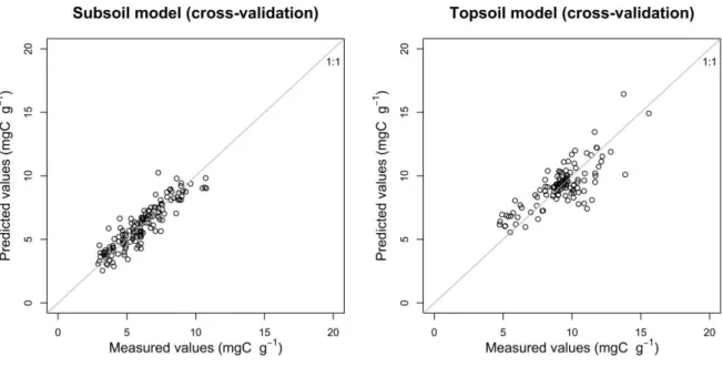
119
trees at all depths. Moreover, our hypothesis was that additional SOC in the agroforestry plot
120
compared to the control plot would enrich all particle-size fractions.
6 2. Materials and methods
122
2.1. Site description
123
The experimental site was located in Prades-le-Lez, 15 km North of Montpellier,
124
France (Longitude 04°01’ E, Latitude 43°43’ N, elevation 54 m a.s.l.). The climate is
sub-125
humid Mediterranean with an average temperature of 14.5°C and an average annual rainfall of
126
951 mm (years 1996–2003). The soil is a silty and carbonated deep alluvial Fluvisol (IUSS
127
Working Group WRB, 2007). From 1950 to 1960, the site was a vineyard (Vitis vinifera L.),
128
and from 1960 to 1985 the field was occupied by an apple (Malus Mill.) orchard. The apple
129
tree stumps were removed in 1985. Then, durum wheat (Triticum turgidum L. subsp. durum
130
(Desf.) Husn.) was cultivated. In February 1995, a 4.6 hectare agroforestry alley-cropping
131
plot was established after the soil was ploughed to 20 cm depth, with the planting of hybrid
132
walnuts (Juglans regia × nigra cv. NG23) at 13 × 4 m spacing, with East–West tree rows
133
(Fig. 1). The remaining part of the plot (1.4 ha) was kept as a control agricultural plot. The
134
walnut trees were planted at an initial density of 200 trees ha-1. They were thinned in 2004
135
down to 110 trees ha-1. In the tree rows, the soil was not tilled and spontaneous herbaceous
136
vegetation grew. The cultivated inter-row was 11 m wide. Since the tree planting, the
137
agroforestry inter-row and the control plot were managed in the same way. The annual crop
138
was most of the time durum wheat, except in 1998, 2001 and 2006, when rapeseed (Brassica
139
napus L.) was cultivated, and in 2010 and 2013, when pea (Pisum sativum L.) was cultivated.
140
The durum wheat crop was fertilized as a conventional crop (120 kg N ha-1 yr-1), and the soil
141
was ploughed annually to 20 cm depth, before durum wheat was sown.
142
143 144 145
7 146
Figure 1. Hybrid walnut-durum wheat agroforestry system. Left panel: in November 2013;
147
Right panel: in June 2014.
148
149
2.2. Soil core sampling
150
The experimental site was not designed as traditional agronomical experiments with blocks
151
and replicates, but with two large adjacent plots. First, soil texture was analyzed for 24
152
profiles down to 2 m soil depth, following a random sampling design within the two plots. In
153
May 2013, a sub-plot of 625 m2 was sampled in both plots, following an intensive sampling
154
scheme (Fig. 2). In the agroforestry plot, this sub-plot included two tree rows, two inter-rows
155
and nine walnut trees. Walnut trees had a mean height of 11.21 ± 0.65 m, a mean height of
156
merchantable timber of 4.49 ± 0.39 m and a mean diameter at breast height of 25.54 ± 1.36
157
cm. Soil cores (n=36) were sampled on a regular grid, every 5 m (Fig. 2). Around each tree, a
158
soil core was collected at 1 m, 2 m and 3 m distance from the tree (n=57), in the tree row and
159
perpendicular to the tree row. Seven soil cores were sampled additionally in the middle of the
160
inter-row to study short scale (1 m distance) spatial heterogeneity of SOC stocks far from the
161
trees (Fig. 2). The same sampling scheme was followed in the control plot without these seven
162
additional soil cores. Thus, 100 soil cores were sampled in the agroforestry sub-plot (40 in
8
tree rows, 60 in inter-rows) and 93 in the agricultural sub-plot (Fig. 2). All cores were
164
sampled down to 2 m depth using a motor-driven micro caterpillar driller (8.5-cm diameter
165
and 1-m long soil probe). The soil probe was successively pushed two times into the soil, to
166
get 0-1 m and 1-2 m cores at each sampling point. Each soil core was then cut into ten
167
segments, corresponding to the following depth increments: 0-10, 10-30, 30-50, 50-70,
70-168
100, 100-120, 120-140, 140-160, 160-180, and 180-200 cm.
169
170
Figure 2. Description of the intensive sampling scheme in the agroforestry and in the control
171
sub-plots. Circles represent hybrid walnuts, the grey strips represents the tree rows,
172
triangles are for soil cores on the regular grid (every 5 m), squares are for soil cores
173
on transects (every 1 m).
174 175
2.3. Use of field visible and near infrared spectroscopy to predict SOC
176
As core surface had been smoothed by the soil probe, each segment was refreshed with
177
a knife before being scanned, in order to provide a plane but un-smoothed surface. Then, four
178
VNIR spectra (from 350 to 2500 nm at 1 nm increment) were acquired in the field at different
9
places of each segment, using a portable spectrophotometer ASD LabSpec 2500 (Analytical
180
Spectral Devices, Boulder, CO, USA), and were then averaged. Reflectance spectra were
181
recorded as absorbance, which is the logarithm of the inverse of reflectance. The whole
182
spectrum population was composed of 1908 mean spectra (i.e. 193 cores with 10 sub-cores
183
per core but a few samples were lost due to mechanical problems). In topsoil (0-30 cm), the
184
soil was dry and crumbled whereas in deeper soil horizons, it was moister and had higher
185
cohesion. Thus, two different predictive models were built: one for topsoil samples, the other
186
for subsoil (30-200 cm) samples. The “topsoil model” for predicting SOC was built using the
187
116 most representative topsoil samples, out of 380 samples, and the “subsoil model”, using
188
the 142 most representative subsoil samples, out of 1488 samples. The procedure to select the
189
most representative samples is presented below. The 0-10 cm soil layer from the tree rows (40
190
samples) was not used for the topsoil model as it contained abundant plant debris < 2 mm
191
(roots, leaves, etc.) and a PCA revealed that these VNIR spectra were different from the
192
whole spectra population. SOC concentration of these samples was therefore determined with
193
a CHN elemental analyzer, and, thus, not predicted by VNIR. The SOC concentration of the
194
258 samples selected for building the VNIR prediction models was also analyzed using a
195
CHN elemental analyzer.
196 197
2.4. VNIR spectra analysis and construction of predictive models
198
VNIR spectra analysis was conducted on topsoil and subsoil samples separately, using
199
the WinISI 4 software (Foss NIRSystems/ Tecator Infrasoft International, LLC, Silver Spring,
200
MD, USA) and R software version 3.1.1 (R Development Core Team, 2013). The most
201
representative samples, from a spectral viewpoint, were selected using the Kennard-Stone
202
algorithm, which is based on distance calculation between sample spectra in the principal
10
component space (Kennard and Stone, 1969). For the topsoil model, the calibration subset
204
included 104 samples (90%) selected as the most representative spectrally, and the validation
205
subset 12 samples (10%). For the subsoil model, the calibration subset included 128 samples
206
(90%), and the validation subset 14 samples. Fitting the spectra to the SOC concentrations
207
determined with a CHN elemental analyzer was performed using partial least squares
208
regression (PLSR; Martens and Naes, 1989). We tested common spectrum preprocessing
209
techniques including first and second derivatives, de-trending, standard normal variate
210
transformation and multiplicative scatter correction, but the best models were obtained when
211
no pre-treatment was applied on the spectra (data not shown). Then cross-validation was
212
performed within the calibration subset, using groups that were randomly selected (10
213
groups), in order to build the model used for making predictions on the samples not analyzed
214
in the laboratory. No outlier was removed. The number of components (latent variables) that
215
minimized the standard error of cross-validation (SECV) was retained for the PLSR. The
216
performance of the models was assessed on the validation subsets using the coefficient of
217
determination (R²) and the standard error of prediction (SEP) between predicted and measured
218
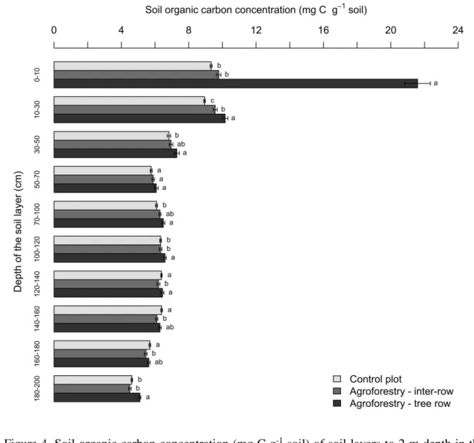
values, and also the ratio of standard deviation to SEP, denoted RPD, and the RPIQ, which is
219
the ratio of performance to IQ (interquartile distance), i.e. IQ/SEP = (Q3 – Q1)/SEP, where
220
Q1 is the 25th percentile and Q3 is the 75th percentile (Bellon-Maurel et al., 2010). Then all
221
sub-set samples (i.e., calibration and validation samples) were used to build models that were
222
applied on the samples not analyzed in the laboratory. The performance of these models was
223
also assessed according to R², SECV, RPD and RPIQ.
224
225 226
11
Table 1. External validation and prediction model results for soil organic carbon. N: numbers of samples; SD: standard deviation (mean and
228
standard deviation of the conventional determinations); R2: coefficient of determination; RPD is the ratio of performance to deviation,
229
i.e. the ratio of SD to SEP or SECV. RPIQ is the ratio of performance to IQ (interquartile distance), i.e. IQ/SEP (or SECV) = (Q3 -
230
Q1)/SEP (or SECV).
231
Topsoil External validation on 10% samples after
calibration using 90% samples
Prediction model using 100% samples (10-group cross-validation) N Mean mg g-1 SD mg g-1 SEP mg g-1 Bias mg g-1 R2 RPD RPIQ N Mean mg g-1 SD mg g-1 SECV mg g-1 R2 RPD RPIQ 12 9.71 2.09 1.04 -0.59 0.78 1.75 2.60 116 9.18 1.99 1.20 0.63 1.66 4.35 Subsoil External validation on 10% samples after
calibration using 90% samples
Prediction model using 100% samples (10-group cross-validation) N Mean mg g-1 SD mg g-1 SEP mg g-1 Bias mg g-1 R2 RPD RPIQ N Mean mg g-1 SD mg g-1 SECV mg g-1 R2 RPD RPIQ 14 6.19 1.80 0.83 0.01 0.74 2.03 3.03 142 6.06 1.86 0.77 0.83 2.40 4.85 232 233
12
Subsoil models performed better than topsoil models (Table 1, Fig. S1). In external
234
validation, RPD was higher than 2 for the subsoil, which has been considered a threshold for
235
accurate NIRS prediction of soil properties in the laboratory (Chang et al., 2001). This RPD
236
threshold was not achieved for the topsoil model, but SOC concentrations were predicted for
237
less than 60% of topsoil samples, the rest was directly analyzed with a CHN elemental
238
analyzer. It is worth noting that cross-validation on the whole set (for making prediction on
239
the samples not analyzed in the lab) yielded better results than external validation (on 10% of
240
analyzed samples) in the subsoil, but the opposite was observed in the topsoil.
241
242
2.5. Bulk densities determination
243
Each segment was weighed in the field to determine its humid mass. Following this
244
step, each segment was crumbled and homogenized, and a representative sub-sample of about
245
300 g was sampled. Sub-samples were sieved at 2 mm to separate coarse fragments such as
246
stones and living roots. Coarse fragments represented less than 1% of each soil mass and were
247
considered as negligible. Moisture contents were determined for 23 soil cores (i.e. 230
248
samples) after 48 h drying at 105°C, and were used to calculate the dry mass of all samples.
249
Bulk density (BD) was determined for each sample by dividing the dry mass of soil by its
250
volume in the soil corer tube.
251 252
2.6. Reference analysis measurements
253
After air drying, soil samples were oven dried at 40°C for 48 hours, sieved at 2 mm,
254
and ball milled until they passed a 200 µm mesh sieve. Carbonates were removed by acid
255
fumigation, following Harris et al., (2001). For this, 30 mg of soil was placed in open Ag-foil
13
capsules. The capsules were then placed in the wells of a microtiter plate and 50 µL of
257
demineralized water was added in each capsule. The microtiter plate was then placed in a
258
vacuum desiccator with a beaker filled with 100 mL of concentrated HCl (37%). The samples
259
were exposed to HCl vapors for 8 hours, and were then dried at 60°C for 48 hours. Capsules
260
were then closed in a bigger tin capsule. Decarbonated samples were analyzed for organic
261
carbon concentration with a CHN elemental analyzer (Carlo Erba NA 2000, Milan, Italy).
262
Isotopic measurements were performed on a few samples to check that decarbonation was
263
well performed (δ13C OM = -25 ‰).
264
265
2.7. Soil organic carbon stock calculation
266
In most studies comparing SOC stocks between treatments or over time periods, SOC
267
stocks have been quantified to a fixed depth as the product of soil bulk density, depth and
268
SOC concentration. However, if soil bulk density differs between the treatments being
269
compared, the fixed-depth method has been shown to introduce errors (Ellert et al., 2002). A
270
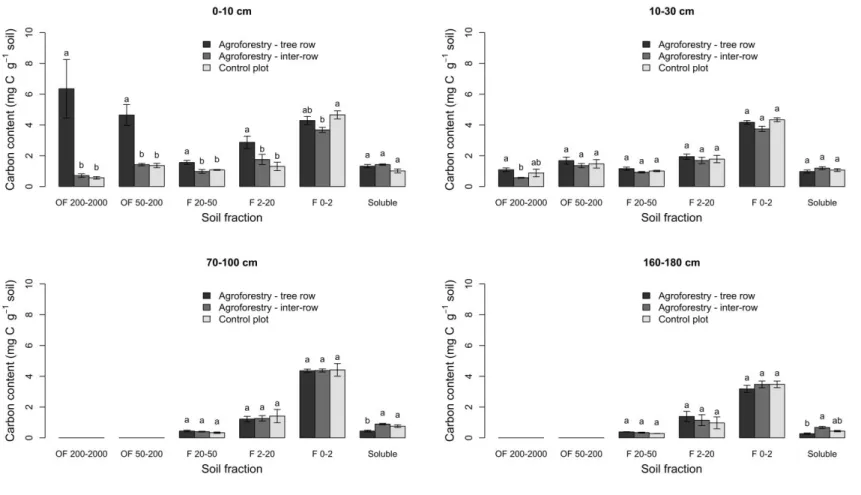
more accurate method is to use an equivalent soil mass (ESM) (Ellert and Bettany, 1995). We
271
defined a reference soil mass profile that was used as the basis for comparison, based on the
272
lowest soil mass observed at each sampling depth and location. For this reference, soil mass
273
layers (0-1000, 1000-4000, 4000-7300, 7300-10700, 10700-15700, 15700-18700,
18700-274
21900, 21900-25100, 25100-28300, 28300-31500 Mg ha−1) corresponded roughly to soil
275
depth layers (0–10, 10–30, 30–50, 50-70, 70-100, 100-120, 120-140, 140-160, 160-180,
180-276
200 cm, respectively). For the different treatments (control, tree row, inter-row), SOC stocks
277
were calculated on this basis, soil mass was the same, whereas depth layer varied (Table 2).
278
The effect of the ESM correction can be seen in Table S1. SOC stocks in the agroforestry plot
279
were calculated with tree rows representing 16% of the plot surface area and inter-rows 84%:
14
SOC stock𝐴𝑔𝑟𝑜𝑓𝑜𝑟𝑒𝑠𝑡𝑟𝑦 = 0.16 × SOC stock𝑇𝑟𝑒𝑒 𝑟𝑜𝑤+ 0.84 × SOC stock𝐼𝑛𝑡𝑒𝑟 𝑟𝑜𝑤 (1)
281
We defined delta SOC stock as the difference between SOC stock in the agroforestry plot and
282
in the control plot:
283
Δ SOC stock = SOC stock𝐴𝑔𝑟𝑜𝑓𝑜𝑟𝑒𝑠𝑡𝑟𝑦− SOC stock𝐶𝑜𝑛𝑡𝑟𝑜𝑙 (2)
284
All SOC stocks were expressed in Mg C ha−1. SOC accumulation rates (kg C ha−1 yr-1) were
285
calculated by dividing delta stocks by the number of years since the tree planting (18 years):
286
SOC accumulation rate =Δ SOC stock
18 × 1000 (3)
287
2.8. Particle-size fractionation
288
Particle-size fractionation was performed for five soil cores from the inter-rows, five from the
289
tree rows and six from the control plot, and at four depths: 0-10, 10-30, 70-100 and
160-290
180 cm. Thus, 64 soil samples were fractionated, as described in Balesdent et al. (1998) and
291
Gavinelli et al. (1995). Briefly, 20 g of 2-mm sieved samples were soaked overnight at 4°C in
292
300 mL of deionized water, with 10 mL of sodium metaphosphate (HMP, 50 g L-1). Samples
293
were then shaken 2 h with 10 glass balls in a rotary shaker, at 43 rpm. The soil suspension
294
was wet-sieved through 200-µm and 50-µm sieves, successively. The fractions remaining on
295
the sieves were density-separated into organic fractions, floating in water, and remaining
296
mineral fractions. The 0-50 µm suspension was ultrasonicated during 10 min with a
probe-297
type ultrasound generating unit (Fisher Bioblock Scientific, Illkirch, France) having a power
298
output of 600 watts and working in 0.7:0.3 operating/interruption intervals. This 0-50 µm
299
suspension was then sieved through a 20-µm sieve. The resulting 0-20 µm suspension was
300
transferred to l-L glass cylinders, which were then shaken by hand and 50 mL of the
301
suspension were withdrawn immediately after. They constituted an aliquot of the entire 0-20
302
µm fraction. After a settling time of 8 h approximately, a second aliquot of 50 mL was
15
removed by siphoning the upper 10 cm of the suspension left after the first sampling. This
304
represented an aliquot of the 0-2 µm fraction. A third aliquot was also collected in the upper
305
10 cm, and centrifuged two times 35 min, at 4000 rpm. This aliquot was then filtered at 2 µm
306
to get the hydrosoluble fraction. Fractions were then dried at 40°C, finely ground,
307
decarbonated and analyzed with a CHN elemental analyzer. A binocular microscope was used
308
to check if separation of coarse mineral fractions and of light organic coarse fractions
(200-309
2000 and 50-200 µm) was well done. No pyrogenic particles were observed. Organic carbon
310
contents of coarse mineral fractions were then assumed to be 0 mg C g-1. A sub-sample of
311
each of the 64 selected samples was used to perform a classical textural analysis after
312
destruction of organic matter. These texture analyses were used to evaluate the quality of the
313
dispersion for soil particle size fractionation.
314
315
2.9. Calculation of SOC saturation
316
The theoretical value of SOC saturation was calculated according to the equation proposed by
317
(Hassink, 1997):
318
𝑆𝑂𝐶𝑠𝑎𝑡−𝑝𝑜𝑡 = 4.09 + 0.37 × particles < 20 μm (4)
319
where SOCsat-pot is the potential SOC saturation (mg C g-1) and where particles < 20 µm 320
represents the proportion of fine soil particles <20 µm (%).
321
To calculate the SOC saturation deficit (Angers et al., 2011; Wiesmeier et al., 2014), the
322
estimated current SOC concentrations of the fine fraction were subtracted from the potential
323
SOC saturation:
324
𝑆𝑂𝐶𝑠𝑎𝑡−𝑑𝑒𝑓 = 𝑆𝑂𝐶𝑠𝑎𝑡−𝑝𝑜𝑡 − 𝑆𝑂𝐶𝑐𝑢𝑟 (5)
16
where SOCsat-def is the SOC saturation deficit (mg C g-1) and SOCcur is the current mean SOC 326
concentration of the fine fraction <20 µm (mg C g-1). The total amount of the SOC storage
327
potential (SOCstor-pot, Mg C ha-1) was calculated multiplying SOCsat-def by soil bulk density and 328
soil layer thickness.
329
These calculations were performed for the four depths where particle-size fractionation was
330
done (0-10, 10-30, 70-100 and 160-180 cm). But as the equation proposed by (Hassink, 1997)
331
was calibrated for topsoil layers, calculations for deep soil layers are only indicative.
332 333
2.10. Statistical analyses
334
The observed variability in a soil property 𝑍 such as SOC concentration results from complex
335
processes operating over various spatial scales. A simple but useful statistical model for 𝑍 at a
336
set of observations that could be spatially located, 𝒔𝑖 = {𝒔 1, 𝒔 2, ⋯ , 𝒔𝑞 } is
337
𝑍(𝒔𝑖 ) = 𝜇(𝒔𝑖 ) + 𝜀(𝒔𝑖 ) (6)
338
where 𝜇(𝒔𝑖 ) is a deterministic component and 𝜀(𝒔𝑖 ) is a correlated random component that
339
can include a pure noise random one. A soil property can be correlated with other
340
environmental variables such as, in this work, the distance to the closest tree. This can be
341
represented in Equation 6 by assuming that 𝜇(𝒔𝑖 ) comprises an additive combination of one
342
or more fixed effect:
343
𝜇(𝒔𝑖 ) = 𝛽0+ ∑𝑞𝑗=1𝛽𝑗𝑥𝑗 (𝒔𝑖 ) (7)
344
where 𝑥𝑗 (𝑗 = 1,2, ⋯ , 𝑞) are 𝑞 auxiliary variables and 𝛽0, … , 𝛽𝑞 are the associated fixed
345
effects. This model is referred as a Mixed Effects Model which offers a flexible framework by
346
which to model the sources of variation and correlation that arise from grouped data (Lark et
17
al., 2006; Pinheiro and Bates, 2000). In this work, we fitted two different linear mixed models
348
(LMM).
349
We first fitted a LMM using the whole set of the bulk densities, SOC concentrations, and
350
SOC stocks observations at the different depths. We used the nlme package (Pinheiro et al.,
351
2013). Soil core ID was considered as a random effect to take into account a sample effect.
352
These soil properties were then compared by depth and per location (control, tree row,
inter-353
row). An ANOVA was performed on these models. We then used the multcomp package
354
(Hothorn et al., 2008) to perform a post hoc analysis and determine which means differed
355
significantly between the control, tree rows and inter-rows, using the Tukey-Kramer test,
356
designed for unbalanced data. To study spatial influence on SOC stocks, “distance to the
357
closest tree” was added to the LMM model, and an ANOVA was performed.
358
Secondly, we fitted a LMM in a geostatistical framework using the cumulated SOC stock
359
observations for 3 depths (0-30 cm, 0-100 cm and 0-200 cm). In a spatial context, the random
360
effects of the LMM describe spatially-correlated random variation. The LMM model is then
361
parameterized by a global vector, called Θ, of model parameters which include the parameters
362
of the covariance function and the fixed effects coefficients. These can be fitted to the data by
363
a likelihood method. Lark et al. (2006) described how the maximum likelihood estimator is
364
biased in the presence of fixed effects and suggested that the restricted maximum likelihood
365
estimator (REML) should be applied. Following Villanneau et al., (2011) we have tested the
366
assumption that the random effects are spatially correlated by comparing the quality of the
367
model-fit for spatially correlated and spatially independent models (usually called pure nugget
368
model). Webster and McBratney, (1989) suggested that the Akaike information criterion
369
(AIC, Akaike, 1974) should be used to compare different spatially correlated models. Once
370
the parameters of the LMM have been fitted, they may be plugged into the best linear
371
unbiased predictor to form the empirical best linear unbiased predictor (E-BLUP) of the
18
property at unsampled sites (Lark et al., 2006). The error variance of the E-BLUP can also be
373
computed at any unsampled site. For this, the value of fixed effects covariates must be known
374
at each prediction site. We therefore calculated several grids of the fixed effects with a 25 cm
375
cell size. The use of any model of spatial variation implies that assumptions have been made
376
about the type of variation the data exhibit. Once the model has been fitted, cross-validation
377
can be used to confirm that these assumptions are reasonable and that the spatial model
378
appropriately describes the variation. We therefore computed a ‘leave-one-out
cross-379
validation’. For each sampling location, 𝒔𝑖 (𝑖 = 1,2, ⋯ , 𝑞), the value of the property at 𝒔𝑖 was
380
predicted by the E-BLUP upon the vector of observations excluding 𝑍(𝒔𝑖 ), in order to
381
compute the standardized squared prediction error (SSPE: the squared difference between the
382
E-BLUP and the observed value divided by the computed prediction error variance (PEV)).
383
Under an assumption of normal prediction errors, the expected mean SSPE is 1.0 if the PEVs
384
are reliable (which requires an appropriate variogram model), and the expected median SSPE
385
is 0.455. The spatial analysis package GeoR (Ribeiro and Diggle, 2001) was used for REML
386
fitting and kriging.
387
Finally, a Kruskal-Wallis test (Kruskal and Wallis, 1952) was performed to analyze SOC
388
concentration in soil fractions per depth and per location (5 or 6 replicates). This test was
389
followed by a post hoc analysis using Dunn’s test (Dunn, 1964) with a Bonferroni correction
390
(p-value=0.017).
391
All the statistical analyses were performed using R software version 3.1.1 (R Development
392
Core Team, 2013), at a significance level of <0.05.
393 394
395 396
19
Table 2. Soil organic carbon stocks (Mg C ha-1) and SOC accumulation rates (kg C ha-1 yr-1). Associated errors are standard errors (40 replicates
397
for the tree-row, 60 replicates for the inter-row, and 93 replicates for the control plot). ESM = Equivalent Soil Mass. Significantly
(p-398
value<0.05) different SOC stocks are followed by different letters.
399
Cumulated ESM (Mg ha-1)
Cumulated calculated depth to ESM (cm)
Cumulated SOC stocks (Mg C ha-1) Δ SOC stocks
(Mg C ha-1)
SOC accumulation rates (kg C ha-1 yr-1)
Tree-row Inter-row Control Tree-row Inter-row Agroforestry Control Δ (Agroforestry
– Control) Agroforestry vs Control Inter-row vs Control 1000 0-9 0-8 0-7 21.6 ± 1.0 a 9.8 ± 0.4 c 11.7 ± 0.3 b 9.3 ± 0.1 c 2.3 ± 0.4 129 ± 20 24 ± 21 4000 0-29 0-27 0-26 52.8 ± 1.4 a 37.9 ± 0.6 c 40.3 ± 0.5 b 35.8 ± 0.2 d 4.5 ± 0.6 248 ± 31 115 ± 33 7300 0-49 0-47 0-45 77.1 ± 1.5 a 62.0 ± 0.7 c 64.4 ± 0.6 b 59.4 ± 0.2 d 5.0 ± 0.6 276 ± 36 141 ± 39 10700 0-69 0-66 0-64 98.1 ± 1.5 a 82.4 ± 0.7 c 84.9 ± 0.6 b 79.7 ± 0.3 d 5.1 ± 0.7 286 ± 39 147 ± 43 15700 0-98 0-95 0-93 130.4 ± 1.5 a 113.7 ± 0.7 c 116.4 ± 0.7 b 110.1 ± 0.3 d 6.3 ± 0.7 350 ± 41 202 ± 45 18700 0-118 0-115 0-112 150.3 ± 1.5 a 133.1 ± 0.8 c 135.9 ± 0.7 b 129.3 ± 0.4 d 6.5 ± 0.8 363 ± 43 210 ± 46 21900 0-137 0-134 0-131 170.9 ± 1.5 a 152.8 ± 0.8 c 155.7 ± 0.7 b 149.5 ± 0.4 c 6.2 ± 0.8 345 ± 44 185 ± 48 25100 0-157 0-154 0-150 191.0 ± 1.6 a 172.4 ± 0.8 c 175.4 ± 0.7 b 169.9 ± 0.4 c 5.5 ± 0.8 306 ± 45 140 ± 49 28300 0-176 0-173 0-170 209.5 ± 1.6 a 190.5 ± 0.8 c 193.5 ± 0.7 b 189.3 ± 0.4 c 4.3 ± 0.8 238 ± 47 69 ± 51 31500 0-196 0-193 0-189 226.1 ± 1.6 a 206.0 ± 0.84 c 209.2 ± 0.7 b 205.9 ± 0.4 c 3.3 ± 0.9 183 ± 48 5 ± 53
20 3. Results
400
3.1. Changes in soil texture with depth
401
Clay, silt and sand profiles were very similar at both plots (Fig. 3). Soil texture was
402
homogeneous in the first 50 cm. Clay and silt contents linearly increased till 100 cm soil
403
depth to reach about 325 g kg-1 and575 g kg-1 respectively, while sand content decreased. Soil
404
texture did not change between 100 and 200 cm soil depth. Below 140 cm depth, clay and
405
sand content were significantly different (F=71.31, P<0.001) in both plots, but the maximum
406
difference was less than 20 g kg-1.
407
408
Figure 3. Changes in soil texture with depth in the control plot and in the agroforestry plot.
409
Error bars represent standard errors (n=100 in the agroforestry, n=93 in the control).
410
411 412
21
3.2. Soil bulk densities
414
Soil bulk densities were significantly higher in the control plot than in the tree row at all
415
depths except for 30-50 and 140-160 cm, and higher than in the inter-row, except for 10-30
416
and below 140 cm depth (Table 3). In the agroforestry system, soil bulk densities were higher
417
in the inter-row than in the tree row for 0-10 and 10-30 cm.
418
419
Figure 4. Soil organic carbon concentration (mg C g-1 soil) of soil layers to 2-m depth in the
420
control plot and in the agroforestry plot. Error bars represent standard errors (n=100
421
in the agroforestry, n=93 in the control). Significantly (p-value<0.05) different SOC
422
concentrations per depth are followed by different letters.
22
Table 3. Mean soil bulk densities (g cm-3). For a given depth, means followed by the same letters do not differ significantly at p = 0.05.
424
Associated errors are standard errors (40 replicates for the tree-row, 60 replicates for the inter-row, and 93 replicates for the control plot).
425 426 427 428 429 430 431 432 433 434
Depth (cm) Agroforestry – tree row Agroforestry – inter-row Control plot 0-10 1.10 ± 0.02 c 1.23 ± 0.03 b 1.41 ± 0.01 a 10-30 1.49 ± 0.01 b 1.60 ± 0.02 a 1.61 ± 0.00 a 30-50 1.71 ± 0.01 ab 1.67 ± 0.02 b 1.73 ± 0.00 a 50-70 1.73 ± 0.01 c 1.77 ± 0.01 b 1.80 ± 0.00 a 70-100 1.68 ± 0.00 c 1.71 ± 0.00 b 1.74 ± 0.00 a 100-120 1.55 ± 0.01 b 1.55 ± 0.01 b 1.61 ± 0.00 a 120-140 1.63 ± 0.00 b 1.64 ± 0.01 b 1.65 ± 0.00 a 140-160 1.64 ± 0.00 a 1.64 ± 0.01 a 1.65 ± 0.00 a 160-180 1.62 ± 0.01 b 1.65 ± 0.01 a 1.65 ± 0.00 a 180-200 1.64 ± 0.00 b 1.65 ± 0.00 a 1.65 ± 0.00 a
23
3.3. Soil organic carbon concentrations
435
An ANOVA performed on the LMM model revealed that soil depth (F-value=270, P<0.0001)
436
and location, i.e., tree row vs. inter-row (F-value=171, P<0.0001), were the only variables
437
affecting significantly SOC concentrations. Distance to the closest tree had no significant
438
effect (F-value=1.3, P=0.28). As shown in Fig. 4, for 0-10 cm, SOC concentration doubled in
439
the tree row (21.6 ± 0.8 mg C g-1) compared to the inter-row (9.8 ± 0.1 mg C g-1) and to the
440
control (9.3 ± 0.1 mg C g-1), whereas the latter two were not significantly different. SOC
441
concentration was significantly higher in the tree row than in the control plot to 120 cm soil
442
depth, except in the 50-70 cm soil layer where no difference was observed. SOC
443
concentration was significantly higher in the tree row than in the inter-row to 30 cm soil
444
depth.
445 446
3.4. Soil organic carbon stocks
447
Fig. 5 represents SOC stocks in the agroforestry plot as a function of soil depth, location and
448
distance to the closest tree. For a given depth and distance to the closest tree, variability of
449
SOC stocks was high, and there was no effect of the distance to the closest tree on SOC stocks
450
(Fig. 5). An ANOVA performed on the LMM model confirmed that SOC stocks were
451
significantly influenced by soil depth (F-value=483, P<0.0001) and location, i.e., tree row vs.
452
inter-row (F-value=66, P<0.0001), but not by the distance to the closest tree (F-value=1.5,
453
P=0.22).
454
For an equivalent soil mass (ESM) of 4000 Mg ha-1 (to 26-29 cm depth), SOC stocks were
455
significantly higher in the tree row than in the inter row and in the control (Table 2). For an
456
ESM of 31500 Mg ha-1 (to 189-196 cm depth), SOC stocks were about 20 Mg C ha-1 higher in
457
the tree rows compared to the inter-rows or to the control. Cumulated SOC stocks were
24
significantly higher in the inter-row than in the control plot to an ESM of 18700 Mg ha-1 (to
459
112-115 cm depth), except for an ESM of 1000 Mg ha-1 where not difference was found
460
(Table 2).
461
At the plot scale, cumulated SOC stocks in the agroforestry plot were significantly higher than
462
in the control plot at all depths (Table 2). For an ESM of 4000 Mg ha-1 (to 26-29 cm depth),
463
SOC stocks were 40.3 ± 0.5 Mg C ha-1 and 35.8 ± 0.2 Mg C ha-1 in the agroforestry and in the
464
control, respectively. For a soil mass of 15700 Mg ha-1 (to 93-98 cm depth), Δ SOC stock
465
between the agroforestry and the control was 6.3 ± 0.7 Mg C ha-1. This difference was much
466
lower without the ESM correction (Table S1).
467 468
3.5. Soil organic carbon accumulation rates
469
Compared to the control, inter-rows accumulated 115 ± 33 kg C ha-1 yr-1 for an ESM of 4000
470
Mg ha-1 (26-29 cm) (Table 2), and 202 ± 45 kg C ha-1 yr-1 for an ESM of 15700 Mg ha-1
(93-471
98 cm). SOC accumulation rates in the agroforestry plot compared to the control were 248 ±
472
31 kg C ha-1 yr-1 for an ESM of 4000 Mg ha-1, 350 ± 41 kg C ha-1 yr-1 an ESM of 15700 Mg
473
ha-1, and 183 ± 48 kg C ha-1 yr-1 an ESM of 31500 Mg ha-1 (Table 2). The additional SOC
474
storage rates for 0-10 cm and 10-30 cm were respectively explained at 80% and 60% by the
475 tree rows. 476 477 478 479 480
25 481
Figure 5. Soil organic carbon stocks (Mg C ha-1) in the agroforestry plot as a function of depth, location (tree row vs. inter-row) and distance to
482
the closest tree. The lines represent the regression lines fitted using soil samples per investigated depth. The gray shades display the
483
prediction confidence interval at the 0.95 level.
26
Table 4. Summary of selected models fitted to the data on cumulated soil organic carbon stocks at 3 depths (0-30 cm, 0-100 cm and 0-200 cm)
485
for the 2 plots, and cross validation. SSPE, standardized squared prediction errors; ME, mean error (Mg C ha-1); RMSQE, root mean
486
squared error (Mg C ha-1); AIC, AIC of the spatially correlated model; AIC.ns, AIC of the non-spatially correlated model; 𝛽
0 and 𝛽1 the
487
fixed effects (Mg C ha-1). Bold characters represent the smallest AIC for each depth. The medians and the mean of the cross validation
488
statistics are within the 95% confidence interval.
489 Depth (cm) Mean SSPE Median SSPE
ME RMQSE AIC AIC.ns 𝛽0 𝛽1 Nugget Sill Range Nugget to Sill ratio Agroforestry 0-30 0.99 0.36 -0.004 20.7 585 583 38.1 14.8 19.7 1.3 15.2 0.94 0-100 0.99 0.45 -0.010 43.3 662 665 114.1 16.4 36.0 16.3 12.8 0.69 0-200 0.98 0.39 0.055 123.1 769 780 207.1 19.4 97.8 79.2 12.9 0.55 Control 0-30 1.01 0.33 0.000 2.6 361 357 35.9 - 2.4 0.2 19.4 0.93 0-100 1.01 0.50 0.061 25.7 578 579 111.2 - 20.2 11.0 12.6 0.65 0-200 0.98 0.40 0.519 57.5 665 681 208.9 - 16.4 85.8 6.3 0.16
27
3.6. Spatial distribution of SOC stocks
490
The AIC (Table 4) of the spatially correlated model were less than that of the spatially
491
uncorrelated model for 2 depths (0-100 cm and 0-200 cm for the agroforestry and the control
492
plots), indicating that spatial correlation should be included in the model of variation. We
493
tested several models of spatial variation and retained the spherical model (Webster and
494
Oliver, 2007). For top soil depth of the two plots (0-30 cm), the AIC of the spatially
495
uncorrelated model was slightly the smallest indicating that the residual variation could be
496
independent once fixed effects had been included in the model. But the difference was very
497
small so we considered the spatially correlated model for the rest of the study. The
cross-498
validation results confirmed the validity of the fitted LMM. The nugget to sill ratio measures
499
the unexplained part of the observed variability. The smallest value was observed for the
0-500
200 cm depth in the control plot and the higher was observed for the 0-30 cm depth in both
501
plots. When mapping the SOC stocks for three fixed depths with the BLUP in the two plots, a
502
clear pattern can be observed in the agroforestry plot, with high SOC stocks in the tree rows
503
(Fig. 6). The fitted fixed effects indicate that, in average, the SOC stocks were 15 to 20 Mg C
504
ha-1 higher in the tree rows to 30 to 200 cm depth (Table 4). At the opposite, the control plot
505
did not exhibit any spatial pattern.
506 507 508 509 510 511 512
28 513
Figure 6. Krieged maps of cumulated soil organic carbon stocks (Mg C ha-1) in the
514
agroforestry and in the control plot.
515 516
29
3.7. Organic carbon distribution in soil fractions
517
An average mass yield of 98% and an average carbon yield of 96% were obtained, showing
518
the quality of the particle size fractionation. Furthermore, the variation between soil texture
519
and soil fractionation was only 5-6% (data not shown). Soil segments used for soil
520
fractionation had similar total SOC concentrations compared to mean SOC concentrations at
521
the same depth (Fig. S2). However, the small differences found between SOC concentrations
522
in the inter row and in the control was not visible with the soil segments used for
523
fractionation.
524
For 0-10 cm depth, the distribution of OC in particle size fractions was strongly modified in
525
the tree rows, with an important increase of C in particulate organic matter (POM) fractions
526
(50-200 µm and 200-2000 µm) compared to the inter-row and to the control (Fig. 7). An
527
increase of C in silt size fractions (2-20 µm and 20-50 µm) of the tree rows compared to the
528
inter row and to the control was also observed. Significantly higher C concentrations in the
529
clay fraction (0-2 µm) were observed in the tree row than in the inter-row (Fig. S3), but it was
530
not the case for the amount of C in the clay fraction per gram of soil (Fig. 7).
531
Similar trends in C distribution in fractions were observed at 130 cm depth compared to
0-532
10 cm, although with much smaller differences (Figs. 7, S3). At deeper depths (70-100 and
533
160-180 cm) there were no differences between the three locations (tree row, inter-row and
534
control) except a lower amount of C in the soluble fraction in the tree row. The potential SOC
535
saturation of particles <20 µm was not reached at any depths (Table 5), and the SOC deficit
536
was high. The saturation capacity was far from being reached, as it amounted 17 to 40% of
537
saturation capacity in the tree rows.
538 539
30 541
Figure 7. Organic carbon contents in each soil fraction (mg C g-1 soil). Error bars represent standard errors (n=6 in the control, n=5 in the
inter-542
row and in the tree row). OF = Organic fraction, F = organo-mineral fraction. 0-2, 2-20, 20-50, 50-200 and 200-2000 represent particle
543
size (µm). Means followed by the same letters do not differ significantly at p=0.017 (Dunn’s test with Bonferroni correction).
31
Table 5. Soil organic carbon saturation of the fractionated soil samples in the agroforestry plot. SOCsat-pot, potential SOC saturation (mg C g-1); 545
SOCcur , current mean SOC concentration of the fine fraction <20 µm (mg C g-1); SOCsat-def , SOC saturation deficit (mg C g-1); SOCstor-pot, 546
total amount of the SOC storage potential (Mg C ha-1). Associated errors are standard errors (n=5). Values of SOC saturation for deep soil
547
layers are only indicative.
548
SOCsat-pot
(mg C g-1)
SOCcur (mg C g-1) SOCsat-def (mg C g-1) SOC𝑐𝑢𝑟
SOC𝑠𝑎𝑡−𝑝𝑜𝑡
SOCstor-pot
(Mg C ha-1) Depth (cm) Agroforestry Tree row Inter-row Tree row Inter-row Tree row Inter-row Agroforestry
0-10 18.0 ± 0.4 7.2 ± 0.3 5.4 ± 0.3 10.3 ± 0.4 13.1 ± 0.4 40% 30% 15.3 ± 0.4 10-30 18.7 ± 0.4 6.1 ± 0.1 5.4 ± 0.1 12.6 ± 0.3 13.3 ± 0.3 33% 29% 41.8 ± 0.9 70-100 32.9 ± 0.8 5.6 ± 0.1 5.6 ± 0.1 26.9 ± 0.7 27.6 ± 0.4 17% 17% 140.7 ± 1.9 160-180 32.0 ± 1.1 4.6 ± 0.2 4.6 ± 0.3 26.8 ± 0.7 28.1 ± 0.9 14% 14% 91.9 ± 2.4
32
3.8. Distribution of additional OC in soil fractions
549
For 0-10 cm depth, the additional OC stored between the tree row and the inter-row was
550
explained at 80% by POM fractions, at 15% by silt size fractions, and at 5% by clay fraction,
551
whereas the additional OC stored between the tree row and the control was explained at 80%
552
by POM and at 20% by silt size fractions (Fig. 7). For 10-30 cm, the additional SOC storage
553
between the tree row and the inter-row was explained at 50% by POM fractions, at 25% by
554
coarse and fine silt fractions, and at 25% by clay fraction (Fig. 7), whereas when comparing
555
the tree row and the control these numbers were of 50% (POM) and 50% (silt).
556 557
4. Discussion 558
4.1. A shallow additional SOC storage
559
Sampling to 2-m soil depth indicated that the 0-30 cm soil layer contained less than 20% of
560
total SOC stocks to 2-m depth, demonstrating the importance of deeper soil layers for storing
561
SOC (Harper and Tibbett, 2013; Jobbagy and Jackson, 2000). SOC stocks observed in 0-30
562
cm, from 36 to 41 Mg C ha-1, were comparable to reported values for the Mediterranean
563
region, i.e., 25 to 50 Mg C ha-1 (Martin et al., 2011; Muñoz-Rojas et al., 2012). Additional
564
SOC storage in the agroforestry system compared to the agricultural system was mainly
565
observed up to 30 cm soil depth in the inter-row and up to 50 cm in the tree row. A
566
companion study at the same site indicated that 60% of additional OM inputs (leaf litter,
567
aboveground and belowground biomass of the natural vegetation in the tree row, tree fine
568
roots) to 2 m depth in the agroforestry plot compared to the control plot were located in the
569
first 50 cm (unpublished data). Even if 50% of tree fine root density was found between 1 and
570
4 m soil depth (Cardinael et al., 2015), it was also proven at this site (Germon et al.,
571
submitted) and at other sites (Hendrick and Pregitzer, 1996) that the turnover rate of fine roots
33
decreased with increasing depth, resulting in low OM inputs in deep soil layers. Time since
573
the tree planting (18 years) is probably not long enough to detect changes in SOC stocks at
574
deeper soil depths considering low organic inputs below 1 m depth. For 2012, organic C input
575
due to tree fine root mortality was estimated to be less than 150 kg C ha-1 for 100-200 cm soil
576
depth. Below 1.2 m soil depth, delta of cumulated SOC stocks between the agroforestry and
577
the control plot decreased, due to higher SOC concentrations and stocks in the control at these
578
depths. These higher SOC concentrations were linked to higher SOC concentrations in the
579
clay fraction. This difference may be due to pre-experimental soil heterogeneity, the soil in
580
the agroforestry plot may have had a lower level of SOC below 1.2 m depth before tree
581
planting. An initial heterogeneity was also proposed by Upson and Burgess (2013) who found
582
higher SOC stocks at depth in a control plot compared to an agroforestry plot in an
583
experimental site in England . This shows the limit of paired comparisons - or synchronic
584
studies - to evaluate SOC changes after land use change (Junior et al., 2013; Olson et al.,
585
2014), and pleads for long-term diachronic studies in agroforestry systems. An alternative
586
explanation could be a positive priming effect, i.e., the acceleration of native SOC
587
decomposition by the supply of fresh organic carbon (Fontaine et al., 2007, 2004) from the
588
trees. However, this seems highly unlikely since positive priming effect could not explain
589
such a high C loss of about 3.2 Mg C ha-1 between 1.2 and 2.0 m soil depth in 18 years, i.e.,
590
about 180 kg C ha-1 yr-1. Another hypothesis to explain higher SOC stocks below 1.2 m depth
591
in the control plot is a different belowground water regime between the two plots. Water table
592
depth at this site is known to be very variable (between 5 to 7 m). A shallower water table in
593
the agroforestry plot compared to the control plot may promote capillary action, and therefore
594
cause wetting-drying cycles that could enhance SOM decomposition in deep soil layers
595
(Borken and Matzner, 2009).
596 597
34
4.2. Tree rows and SOC storage in agroforestry systems
598
The high SOC stocks observed in tree rows accounted for an important part of SOC stocks of
599
the agroforestry plot even though tree rows only represented 16% of the surface area. In a
600
poplar (Populus L.) silvoarable agroforestry experiment in England, Upson and Burgess,
601
(2013) also found that the SOC concentration was greater in the top 40 cm under the tree row
602
(19.6 mg C g−1) in the agroforestry treatment than in the cropped alleys (17 mg C g−1), or the
603
arable control (17.1 mg C g−1). Tree rows are comparable to a natural permanent pasture with
604
trees, given that spontaneous herbaceous vegetation grows and that the soil is not tilled.
605
Conversion of arable lands to permanent grasslands is recognized as an efficient land use for
606
climate change mitigation (Soussana et al., 2004). Grasslands can accumulate SOC at a very
607
high rate. For instance, it was estimated on about 20 years old field experiments that
608
conversion from crop cultivation to pasture stored SOC at a rate of 1.01 Mg C ha-1 yr-1 in 0-30
609
cm(Conant et al., 2001). In our case, SOC accumulation rate in the tree rows was 0.94 ± 0.09
610
Mg C ha-1 yr-1 in 0-30 cm. Management of tree rows could therefore have an important role in
611
improving agroforestry systems in terms of SOC storage. Improved grass species could be
612
sown in the tree rows, as well as shrubs between trees. Further research should focus on this
613
aspect to evaluate benefits in terms of SOC storage and biodiversity for instance.
614 615
4.3. Homogeneous distribution of SOC stocks in the cropped alley
616
There was no significant effect of the distance to the trees on SOC stocks at all depths, either
617
in the tree row or in the inter-row. This was also indicated by the maps of the SOC stocks.
618
Tree density was high at this site, and walnuts were about 13 m in height, which is also the
619
distance between two tree rows. This could explain the homogeneous distribution of leaf
620
litterfall observed in the plot (personal observation). In a similar agroforestry system in terms
35
of tree density in Canada, Bambrick et al., (2010) and Peichl et al., (2006) also found no
622
effect of the distance to the trees on SOC stocks to 20 cm depth. They also suggested that the
623
18 m high poplar trees distributed litterfall equally in the crop alleys. Close to the tree rows (1
624
to 2 m distance), the intercrop had a lower yield (15% less in 2012) compared to the middle of
625
the inter-row at the study site (Dufour et al., 2013). On the contrary, tree fine root density was
626
higher close to the tree rows (2.79 t DM ha-1 between 0 and 1.5 m from the tree row in the
627
inter row, and to 4-m soil depth) than in the middle of the inter-rows (1.32 t DM ha-1 between
628
3 and 4.5 m from the tree row in the inter row, and to 4-m soil depth) (Cardinael et al., 2015).
629
Thus, lower carbon inputs from crop residues close to the tree rows may be counterbalanced
630
with higher inputs from tree fine root mortality, explaining homogeneous distribution of SOC
631
stocks within the inter-row (Bambrick et al., 2010; Peichl et al., 2006). In the tree row,
632
homogeneous distribution of SOC stocks may be explained by the short distance between
633
trees and by the presence of abundant herbaceous vegetation.
634 635
4.4. Agroforestry systems: an efficient land use to improve SOC stocks
636
Compared to other agroforestry systems having about the same tree density, a lower SOC
637
accumulation rate in 0-30 cm (0.25 Mg C ha-1 yr-1) was observed at our site. Peichl et al.
638
(2006) reported a SOC accumulation rate of 1.04 Mg C ha-1 yr-1 (0-20 cm) in a 13-year old
639
temperate barley (Hordeum vulgare L.)-poplar intercropping system (111 trees ha-1). In a
21-640
year old agroforestry system in Canada where poplars were intercropped with a rotation of
641
wheat (Triticum aestivum L.), soybean (Glycine max (L.) Merr.) and corn (Zea mays L.),
642
Bambrick et al. (2010) estimated a SOC accumulation rate of 0.30 Mg C ha-1 yr-1 (0-20 cm).
643
Our lower accumulation rate may be explained by warmer climate, higher temperatures
644
enhancing OM decomposition (Hamdi et al., 2013). Moreover, valuable hardwood species
36
like walnut trees have a slower growing rate than fast growing species like poplar (Teck and
646
Hilt, 1991), and therefore for a same tree age, the amount of OC inputs (leaflitter, fine roots)
647
to the soil is lower for slow growing species.
648
Together with other climate-smart farming practices (Lipper et al., 2014), alley-cropping
649
agroforestry systems have the potential to enhance SOC stocks and to contribute to climate
650
change mitigation (Nair et al., 2010; Pellerin et al., 2013). No-till farming is a commonly
651
cited agricultural practice supposed to have a positive impact on SOC stocks. But recent
meta-652
analyses showed this practice had no effect on SOC stocks to 40 cm depth (Luo et al., 2010)
653
or a smaller one (0.23 Mg C ha-1 yr-1 to 30 cm depth) than previously estimated (Virto et al.,
654
2011). A meta-analysis also revealed that the inclusion of cover crops in cropping systems
655
could accumulate SOC at a rate of 0.32 ± 0.08 Mg C ha-1 yr-1 to a depth of 22 cm (Poeplau
656
and Don, 2015). At our site, we found a mean SOC accumulation rate of 0.13 in 0-30 cm in
657
the inter-rows compared to the control. This rate reached 0.25 Mg C ha-1 yr-1 for the whole
658
agroforestry system. A companion study at this site estimated that the tree aboveground C
659
stock was 117± 21 kg C tree-1 (unpublished data). With 110 trees ha-1, total organic carbon
660
(SOC to 1 m soil depth + aboveground tree C) accumulation rate was 1.11 ± 0.13 Mg C ha-1
661
yr-1, making agroforestry systems a possible land use to help mitigating climate change (Lal,
662
2004; Lorenz and Lal, 2014).
663
664
4.5. A long-term SOC storage?
665
Most of additional SOC in the agroforestry plot compared to the control plot was located in
666
coarse soil fractions (50-200 µm and 200-2000 µm). These soil fractions are assumed to
667
contain labile fractions (Balesdent et al., 1998), that are not stabilized by interaction with
668
clays and thus prone to be decomposed by soil microorganisms. Our site might not be old