HAL Id: hal-02962091
https://hal.archives-ouvertes.fr/hal-02962091
Submitted on 8 Oct 2020
HAL is a multi-disciplinary open access
archive for the deposit and dissemination of
sci-entific research documents, whether they are
pub-lished or not. The documents may come from
teaching and research institutions in France or
abroad, or from public or private research centers.
L’archive ouverte pluridisciplinaire HAL, est
destinée au dépôt et à la diffusion de documents
scientifiques de niveau recherche, publiés ou non,
émanant des établissements d’enseignement et de
recherche français ou étrangers, des laboratoires
publics ou privés.
Distributed under a Creative Commons Attribution| 4.0 International License
Cool stars in the Galactic center as seen by APOGEE
M. Schultheis, A. Rojas-Arriagada, K. Cunha, M. Zoccali, C. Chiappini, G.
Zasowski, A. B. A. Queiroz, D. Minniti, T. Fritz, D. A. García-Hernández, et
al.
To cite this version:
M. Schultheis, A. Rojas-Arriagada, K. Cunha, M. Zoccali, C. Chiappini, et al.. Cool stars in the
Galactic center as seen by APOGEE: M giants, AGB stars, and supergiant stars and candidates.
As-tronomy and Astrophysics - A&A, EDP Sciences, 2020, 642, pp.A81. �10.1051/0004-6361/202038327�.
�hal-02962091�
https://doi.org/10.1051/0004-6361/202038327 c M. Schultheis et al. 2020
Astronomy
&
Astrophysics
Cool stars in the Galactic center as seen by APOGEE
M giants, AGB stars, and supergiant stars and candidates
M. Schultheis
1, A. Rojas-Arriagada
2,3, K. Cunha
4,5, M. Zoccali
2,3, C. Chiappini
6,7, G. Zasowski
8,
A. B. A. Queiroz
6,7, D. Minniti
9,3,10, T. Fritz
11,12, D. A. García-Hernández
11,12, C. Nitschelm
13, O. Zamora
11,12,
S. Hasselquist
8,?, J. G. Fernández-Trincado
14, and R. R. Munoz
151 Université Côte d’Azur, Observatoire de la Côte d’Azur, Laboratoire Lagrange, CNRS, Blvd de l’Observatoire, 06304 Nice, France
e-mail: mathias.schultheis@oca.eu
2 Instituto de Astrofísica, Facultad de Física, Pontificia, Universidad Católica de Chile, Av. Vicuña Mackenna 4860, Santiago, Chile
3 Millennium Institute of Astrophysics, Av. Vicuña Mackenna 4860, 782-0436 Macul, Santiago, Chile
4 University of Arizona, Tucson, AZ 85719, USA
5 Observatório Nacional, Sao Cristóvao, Rio de Janeiro, Brazil
6 Leibniz-Institut für Astrophysik Potsdam (AIP), An der Sternwarte 16, 14482 Potsdam, Germany
7 Laboratório Interinstitucional de e-Astronomia, – LIneA, Rua Gal. Joseé Cristino 77, Rio de Janeiro, RJ 20921-400, Brazil
8 Department of Physics & Astronomy, University of Utah, Salt Lake City, UT 84112, USA
9 Departamento de Ciencias Fisicas, Facultad de Ciencias Exactas, Universidad Andres Bello, Av. Fernandez Concha 700,
Las Condes, Santiago, Chile
10 Vatican Observatory, V00120 Vatican City State, Italy
11 Instituto de Astrofísica de Canarias, Calle Via Láctea s/n, 38206 La Laguna, Tenerife, Spain
12 Universidad de La Laguna (ULL), Departamento de Astrofísica, 30206 La Laguna, Tenerife, Spain
13 Centro de Astronomía (CITEVA), Universidad de Antofagasta, Avenida Angamos 601, Antofagasta 1270300, Chile
14 Instituto de Astronomía y Ciencias Planterias, Universidad de Atacama, Copayapu 485, Copiapó, Chile
15 Departamento de Astronomia, Universidad de Chile, Camino El Observatorio 1515, Las Condes, Santiago, Chile
Received 3 May 2020/ Accepted 22 August 2020
ABSTRACT
The Galactic center region, including the nuclear disk, has until recently been largely avoided in chemical census studies because of extreme extinction and stellar crowding. Large, near-IR spectroscopic surveys, such as the Apache Point Observatory Galactic Evolution Experiment (APOGEE), allow the measurement of metallicities in the inner region of our Galaxy. Making use of the latest APOGEE data release (DR16), we are able for the first time to study cool Asymptotic Giant branch (AGB) stars and supergiants in this region. The stellar parameters of five known AGB stars and one supergiant star (VR 5-7) show that their location is well above the tip of the red giant branch. We studied metallicities of 157 M giants situated within 150 pc of the Galactic center from observations obtained by the APOGEE survey with reliable stellar parameters from the APOGEE pipeline making use of the cool star grid down to 3200 K. Distances, interstellar extinction values, and radial velocities were checked to confirm that these stars are indeed situated in the Galactic center region. We detect a clear bimodal structure in the metallicity distribution function, with a dominant metal-rich
peak of [Fe/H] ∼ +0.3 dex and a metal-poor peak around [Fe/H] = −0.5 dex, which is 0.2 dex poorer than Baade’s Window. The
α-elements Mg, Si, Ca, and O show a similar trend to the Galactic bulge. The metal-poor component is enhanced in the α-elements, suggesting that this population could be associated with the classical bulge and a fast formation scenario. We find a clear signature
of a rotating nuclear stellar disk and a significant fraction of high-velocity stars with vgal> 300 km s−1; the metal-rich stars show a
much higher rotation velocity (∼200 km s−1) with respect to the metal-poor stars (∼140 km s−1). The chemical abundances as well as
the metallicity distribution function suggest that the nuclear stellar disk and the nuclear star cluster show distinct chemical signatures
and might be formed differently.
Key words. Galaxy: bulge – Galaxy: stellar content – stars: fundamental parameters – stars: abundances
1. Introduction
The Milky Way bulge is such a complex system that its forma-tion and evoluforma-tion are still poorly understood. As a result of high extinction and crowding, the study of the Galactic bulge
remains challenging. Extinction of more than 30 mag in AV in
the Galactic center (GC) regions requires IR spectroscopy. While an increasing number of detailed chemical abundances in the intermediate and outer bulge (such as Baade’s Window) are now available thanks to large spectroscopic surveys such as ARGOS
? NSF Astronomy and Astrophysics Postdoctoral Fellow.
(Freeman et al. 2013), Gaia-ESO (Rojas-Arriagada et al. 2014),
and APOGEE (García Pérez et al. 2013), chemical abundances
of stars in the inner Galactic bulge (IGB) with projected
dis-tances of RG≤ 200 pc from the GC remain poorly studied.
There have been a few earlier works dedicated to study-ing the chemistry of stars in the central part of the Milky Way. Using high-resolution IR spectra (R ∼ 40 000),Carr et al.(2000) made the first detailed abundance measurement of a star in the GC within 1 pc, the M2 supergiant IRS 7, finding roughly solar metallicity and an abundance pattern that was consistent with
the dredge-up of CNO cycle products. Ramírez et al. (2000)
also analyzed high-resolution IR spectra (R = 40 000) of a
Open Access article,published by EDP Sciences, under the terms of the Creative Commons Attribution License (https://creativecommons.org/licenses/by/4.0),
sample of ten cool supergiant and red-giant stars in the GC
and estimated an iron abundance of +0.12 ± 0.22 dex.
Subse-quently,Cunha et al.(2007) used R ∼ 50 000 spectra to study
the detailed chemistry of the Ramírez et al.(2000) sample and
found a slightly enhanced and narrow metallicity distribution
(h[Fe/H]i= +0.14 ± 0.06 dex) that was also alpha enhanced; we
note that this small sample of 10 stars, save for one, were mem-bers of the central cluster. More recently, Ryde & Schultheis
(2015, RS2015) studied nine field stars with projected distances of R ≤ 50 pc and also found a metal-rich population with
[Fe/H] = +0.11 ± 0.15 dex and a lack of a metal-poor
popu-lation (similarly toCunha et al. 2007), but found low [α/Fe] val-ues, except for calcium. Their mean metallicities are ∼0.3 dex higher than fields in the inner bulge (Rich et al. 2007,2012), indicating that the GC region contains a distinct population. A refined analysis (Nandakumar et al. 2018) gave a slightly higher
mean metallicity of [Fe/H] = +0.3 ± 0.10 dex and confirmed
the very narrow distribution.Grieco et al.(2015) compared these data with a chemical evolution model and concluded that in order to reproduce the observed [α/Fe] ratios, the GC region should have experienced a main strong burst of star formation and should have evolved very quickly with an IMF containing more massive stars.
More recently,Schultheis et al.(2019) found evidence of a
chemically distinct population in the nucleus (nuclear stellar disk (NSD) and nuclear star cluster (NSC)) compared to the IGB that shows a very high fraction of metal-rich stars (∼80%) with a
mean metallicity of+0.2 dex in the GC. They concluded that the
nucleus mimics a metallicity gradient of ∼ −0.27 dex kpc−1 in
the inner 600 pc but is flat if the GC is excluded.
Schultheis et al.(2015) (hereafter referred to as S15) studied 33 M giant stars of APOGEE in the so-called GALCEN field to study the metallicity distribution function and chemical abun-dances using the DR12 data release (Alam et al. 2015). However, they had to limit their analysis to stars with Teff > 3700 K, due
to problems modeling the coolest stars (Holtzman et al. 2015),
thus excluding a large number of cool stars (including asymp-totic giant branch stars (AGB) and supergiants) from their anal-ysis. They found some evidence of the presence of a metal-poor fraction of stars that are α-enhanced.
In this paper, we take advantage of the recently released and
improved results from APOGEE DR16 (Ahumada et al. 2020),
which has several improvements over previous data releases, in particular DR12 (see details inJönsson et al. 2020), and includes additional observations of one plate at APOGEE-S that is ded-icated to observations of targets in the GC. It is most relevant to the study of cool luminous stars in the central parts of the
Milky Way that the DR16 results now cover effective
temper-atures as low as 3200 K using the grid of spherical MARCS
model atmospheres (Gustafsson et al. 2008). In this paper, we
present results for the metallicity distribution function and chem-ical abundances of 157 M giants, which constitutes one of the largest high-resolution spectroscopic samples in the inner degree of the Milky Way to date. In addition, this is the first study of cool AGB stars and supergiants in the GALCEN field using results from the APOGEE survey.
2. The sample 2.1. APOGEE
The Apache Point Observatory Galactic Evolution Experiment (APOGEE) is a large scale, near-IR high-resolution (R ∼ 22 500)
spectroscopic survey of the Milky Way stellar populations,
which is mainly focused on red giants (Majewski et al. 2017;
Zasowski et al. 2013, 2017). APOGEE has been a
compo-nent of both SDSS-III and SDSS-IV (Eisenstein et al. 2011;
Blanton et al. 2017) and uses custom-built twin spectrographs at the Apache Point Observatory’s 2.5 m Sloan Telescope and Las
Campanas Observatory’s 2.5 m du Pont telescope (Gunn et al.
2006; Wilson et al. 2019). APOGEE observes in the H-band, where extinction by dust is significantly lower than at optical wavelengths (e.g., A(H)/A(V) ∼ 0.16).
With its high resolution and high S/N (∼100 per
Nyquist-sampled pixel), APOGEE determines both accurate radial
veloc-ities (better than 0.5 km s−1) and reliable abundance
measure-ments, including the most abundant metals in the universe (C, N, O), along with other α, odd-Z, and iron-peak elements. The
lat-est SDSS-IV data release (DR16;Ahumada et al. 2020) provides
the scientific community with spectra of more than 430 000 stars, as well as the derived stellar properties, including radial veloc-ities, effective temperatures, surface gravities, metallicities, and individual abundances. Additional information, such as photom-etry and target selection criteria, is also provided and described inZasowski et al.(2013,2017). Stellar parameters and chemical abundances for up to 24 elements were derived by the APOGEE Stellar Parameters and Chemical Abundances Pipeline (ASP-CAP, García Pérez et al. 2016), while in Nidever et al. (2015) the data reduction and radial velocity pipelines are described. The model grids are based on a complete set of MARCS stellar atmospheres (Gustafsson et al. 2008), and the spectral synthesis using the Turbospectrum code (Alvarez & Plez 1998,Plez 2012) with a new updated line list has been used (Smith et al., in prep.). In addition to DR16, we use additional observations includ-ing additional stars observed after those released in DR16 from APOGEE-S. These data were reduced with the same pipeline as the DR16 stars.
2.2. Distances
We obtained the StarHorse (SH) distances from Queiroz et al.
(2020a) for the latest APOGEE-2 survey data release DR16, as well as for the additional stars not present in DR16. The SH is a Bayesian fitting code that derives distances and extinc-tion as well as other quantities such as ages and masses. For more details about the method, the priors, and its validation, we refer the reader toQueiroz et al.(2018,2020a) which com-bines the ASPCAP stellar parameters with Gaia DR2 and pho-tometric surveys thus achieving precise distances and extinction; the extinction treatment has been significantly improved in the updated version. The typical internal precision in distance for our GALCEN DR16 sample is about 10 ± 7%. The SH uses
the APOGEE targeting extinction estimate (seeZasowski et al.
2013,2017) as a prior for the total line-of-sight extinction. In addition, we also did a comparison with the 3D extinction map ofSchultheis et al.(2014) using VVV data and the 2D extinction map ofGonzalez et al.(2012), where we find similar AK values
(within 10% uncertainty) with respect to RJCE.
2.3. The GALCEN field
Two plates of GALCEN, one at APO (location ID 4330) and one at LCO (location ID 5534), have been observed with a total num-ber of 619 stars. Due to the high interstellar extinction, a special target selection procedure was applied for the GALCEN field
(Zasowski et al. 2013). Known AGB long-period variables based
on K-band light curves (Matsunaga et al. 2009) were targeted,
as well as spectroscopically identified supergiants such as IRS7, IRS19, and IRS22, and supergiant candidates based on photo-metric color-color criteria. These AGB and supergiant targets have among the coolest effective temperatures (Teff < 3500 K)
in the APOGEE stellar sample. While inS15due to the
limit-ing ATLAS9 model atmospheres grid in ASPCAP for cool stars,
only 33 warm K/M giants were used, for this paper we made
use of the cooler model grid of MARCS model atmospheres to quadruple the sample.
One of the most significant improvements of DR16 com-pared to DR14 is the accuracy and consistency of the derived stellar parameters for the coolest giants (Teff < 3500 K), which
is due to the use of MARCS model atmospheres in spheri-cal symmetry. This improvement can be clearly seen by the
visual inspection of the HR diagram (see e.g., Fig. 3), and
notably the “clumpiness” of the HR diagram with Teff < 3500 K
seen in DR14 is now gone (seeJönsson et al. 2020). However,
“external” calibrators for these cool stars are lacking, which would be important for estimating the accuracy of the stellar parameters for those objects.
For our selection, we disregarded stars with
ASP-CAPFLAGS==’STAR’BAD” and STARFLAGS =
“PERSIST-HIGH”, as well as telluric standard stars, leaving us with a total number of 270 stars. Those 270 include five known AGB stars
and one supergiant star (VR 5-7) in our sample. TableA.1shows
the stellar parameters for those stars.
From the 270 stars, AGB/supergiant candidates have been
chosen as those brighter than H < 12.2, 1.3 < H − K < 3.7,
which excludes AGB/supergiant stars with strong IR excess,
and K0 = K − (1.82 ∗ ((H − K) − 0.2)) < 4.7, which
is the dereddened magnitude to put the star above the AGB tip. We note that the more massive (>3–4 solar masses) and O-rich AGB stars can be brighter (because of flux contribu-tion by hot bottom burning) than the AGB theoretical
luminos-ity limit (see e.g., García-Hernández et al. 2009), and that to
unambiguously distinguish between AGB or supergiant status,
one would need to have photometric light curves and/or some
key chemical information from optical spectra (e.g., lithium and s-process elements;García-Hernández et al. 2006,2007, see also
García-Hernández 2017 for a review). The factor 1.82 corre-sponds to the AK/E(H − K) ratio fromIndebetouw et al.(2005).
The 15 AGB/supergiant candidate stars in our final sample,
together with their stellar parameters, are given in Table2.
Figure 1 shows the dereddened color-magnitude diagram
of the full GALCEN sample, together with the known
AGB/supergiant stars and candidate AGB/supergiant stars,
col-ored by the galactocentric radius. As AGB stars and supergiants have circumstellar material due to their mass-loss, the deredden-ings of those stars were obtained by obtaining the median E(J −
K) color excess from the VVV extinction map (Gonzalez et al.
2012) instead of the APOGEE estimate. Clearly visible is the
foreground contribution with (J − K)0 < 0.8, which can easily
be removed by a simple distance cut. The AGBs and supergiants (both known and candidates) are the most luminous stars and they lie well above the tip of the red giant branch (RGB) with K0= 7.9 (Habing & Olofsson 2004), as indicated by the dashed
line. By imposing a cut-off in RGC< 3.5 kpc, a total of 157 stars
are left over for our analysis. We refer to this later on as the GALCEN sample.
Figure 2 shows the spatial distribution of the GALCEN
sample in Galactic coordinates superimposed on the interstellar extinction map ofGonzalez et al.(2012). In the highest extincted
Table 1. Known AGB and supergiants with stellar parameters from APOGEE-DR16.
2MASS ID Teff log g [M/H] Ref.
2M17451937-2914052 3730 0.34 −0.28 A58(1)
2M17445261-2914110 3244 0.12 0.13 A20(1)
2M17452187-2913443 3290 0.38 0.21 A62(1)
2M17460808-2848491 3555 0.43 −0.46 V5009Sgr(2)
2M17461658-2849498 3242 0.12 −0.15 VR 5-7(3,4)
References. (1) Schultheis et al.(2003), (2)Matsunaga et al. (2009),
(3)Davies et al.(2009), (4)Cunha et al.(2007). Table 2. Supergiant candidates.
2MASS ID Teff log g [M/H] 2M17460746-2846416 3584 0.95 0.29 2M17461382-2825206 3741 0.86 −0.24 2M17461772-2841159 3221 −0.02 −0.12 2M17462661-2819422 3218 −0.38 −0.26 2M17463072-2850325 3327 0.31 0.13 2M17463266-2837184 3692 0.55 −0.11 2M17463693-2820212 3346 0.90 0.13 2M17463769-2841257 3129 −0.15 −0.08 2M17464409-2817487 3128 −0.14 −0.05 2M17464864-2818274 3181 0.35 0.40 2M17471240-2838377 3536 0.31 −0.59 2M17472459-2822320 3337 0.03 −0.09 2M17472709-2840356 3360 0.23 −0.05 2M17480017-2821058 3292 0.23 0.13 ● ● ● ● ● ● ● ● ● ● ● ● ● ● ● ● ● ● ● ● ● ● ● ● ● ● ● ● ● ●● ● ● ● ● ● ● ● ● ● ● ● ● ● ● ● ● ● ● ● ● ● ● ● ● ● ● ● ● ● ● ● ●● ● ● ● ● ● ● ● ● ● ● ● ● ● ● ● ● ● ● ● ● ● ● ● ● ● ● ● ● ● ● ● ●● ● ● ● ● ● ● ● ● ● ● ● ● ● ● ● ● ● ● ● ● ● ● ● ● ● ● ● ● ● ● ● ● ● ● ● ● ● ● ● ● ● ● ● ● ● ● ● ● ● ● ● ● ● ● ● ● ● ● ● ● ● ● ● ● ● ● ● ● ● ● ● ● ● ● ● ● ●● ● ● ● ● ● ● ● ● ● ● ● ● ● ● ● ● ● ● ● ● ● ●● ● ● ● ● ● ● ● ● ● ● ● ● ● ● ● ● ● ● ● ● ● ● ● ● ● ● ● ● ● ● ● ● ● ● ● ● ● ● ● ● ● ● ● ● ● ● ● ● ● ●● ● ● ● ● ● ● ● ● ● ● ● ● ● ● ● ● ● ● ● ● ● ● ● ● ● ● ● ● ● ● ● ● ● ● ● ● ● ● ● ● ● ● ● ● ● ● ● ●● ● ● ● ● ● ● ● ● ● ● ● ● ● ● ● ● ● ● ● ● ● ● ● ● ● ● ● ● ● ● ● ●● ● ● ● ● ● ● ● ● ● ● ● ● ● ● ● ● ● ● ● ● ● ● ● ● ● ● ● ● ● ● ● ●● ● ● ● ● ● ● ● ● ● ● ● ● ● ● ● ● ● ● ● ● ● ● ● ● ● ● ● ● ● ● ● ● ● ● ● ● ● ● ● ● ● ● ● ● ● ● ● ● ● ● ● ● ● ● ● ● ● ● ● ● ● ● ● ● ● ● ● ● ● ● ● ● ● ● ● ● ●● ● ● ● ● ● ● ● ● ● ● ● ● ● ● ● ● ● ● ● ● ● ●● ● ● ● ● ● ● ● ● ● ● ● ● ● ● ● ● ● ● ● ● ● ● ● ● ● ● ● ● ● ● ● ● ● ● ● ● ● ● ● ● ● ● ● ● ● ● ● ● ● ●● ● ● ● ● ● ● ● ● ● ● ● ● ● ● ● ● ● ● ● ● ● ● ● ● ● ● ● ● ● ● ● ● ● ● ● ● ● ● ● ● ● ● ● ● ● ● ● ● ● ● ● ● ● ● ● ● ● ● ● ● ● ● ● ● ● ● ● ● ● ● ● ● ● ● ● ● ● ● ● ● ● ● ● ● ● ● ● ● ● ● ● ● ● ● ● ● ● ● ● ● ● ● ● ● ● ● ● ● ● ● ● ● ● ● ● ● ● ● ● ● ● ● ● ● ● ● ● ● ● ● ● ● ● ● ● ● ● ● ● ● ● ● ● ● ● ● ● ● ● ● ● ● ● ● ● ● ● ● ● ● ● ● ● ● ● ● ● ● ● ● ● ● ● ● ● ● ● ● ● ● ● ● ● ● ● ● ● ● ● ● ● ● ● ● ● ● ● ● ● ● ● ● ● ● ● ● ● ● ● ● ● ● ● ● ● ● ● ● ● ● ● ● ● ● ● ● ● ● ● ● ● ● ● ● ● ● ● ● ● ● ● ● ● ● ● ● ● ● ● ● ● ● ● ● ● ● ● ● ● ● ● ● ● ● ● ● ● ● ● ● ● ● ● ● ● ● ● ● ● ● ● ● ● ● ● ● ● ● ● ● ● ● supergiant AGB supergiant candidates RGB tip 5.0 7.5 10.0 0 2 4
(J−K)
0K
0Fig. 1.Dereddened color-magnitude diagram of the GALCEN sam-ple as a function of the galactocentric distance. Superimposed are known AGB stars (filled circles), known supergiants (filled triangles) and AGB/supergiant candidates (asterisks) based on photometric selec-tion criteria (see text).
● ● ● ● ● ● ● ● ● ● ● ● ● ● ● ● ● ● ● ● ● ● ● ● ● ● ● ● ● ● ● ● ●● ● ●●● ●●● ● ● ● ● ● ● ● ● ● ● ● ● ●●● ● ● ● ● ● ● ● ● ● ● ● ● ● ● ● ● ● ● ● ● ● ● ● ● ● ● ● ● ● ● ● ● ● ● ● ● ● ● ● ● ● ● ● ● ● ● ● ● ● ● ● ● ● ● ● ● ● ● ● ● ● ● ● ● ● ● ● ● ● ● ● ● ● ● ● ● ● ● ● ● ● ● ● ● ● ● ● ● ● ● ● ●● ● ● ● ● ● ● ● ● ● ● ● ● ● ● ● ● ● ● ●● ● ● ● ● ● ● ● ●● ● ● ● ● ● ● ● ● ● ● ● ● ● ● ● ●● ● ● ● ● ● ● ● ● ● ● ● ● ● ● ● ● ● ● ● ● ● ● ● ● ● ● ● ● ● ● ● ● ● ● ● ● ● ● ●● ● ● ● ● ● ● ● ● ● ● ● ● ● ● ● ● ● ● ● ● ● ● ● ● ● ● ● ● ● ● ● ● ● ● ●● ● ●● ● ●● ● ● ● ● ● ● ● ● ● ● ● ● ● ● ● ● ● ● ● ● ● ●● ● ●●●●●●●●●●●●●●●●●●●●●●●●●●● ●●●●●●●●●●●●●●●●●●●● ●●●●●●●●●●●●●● ●●●●●●●●●●● ●●●●●●●●●● ●●●●●●●●● ●●●●●●●● ●●●●●●●● ●●●●●●● ●●●●●●● ●●●●●●● ●●●●●● ●●●●●● ●●●●●● ●●●●●● ●●●●● ●●●●●● ●●●●● ●●●●● ●●●●● ●●●●● ●●●●● ●●●●● ●●●●● ●●●●● ●●●●● ●●●● ●●●●● ●●●●● ●●●● ●●●●● ●●●●● ●●●● ●●●●● ●●●●● ●●●● ●●●●● ●●●● ●●●●● ●●●●● ●●●● ●●●●● ●●●●● ●●●● ●●●●● ●●●●● ●●●●● ●●●●● ●●●●● ●●●●● ●●●●● ●●●●● ●●●●● ●●●●●● ●●●●● ●●●●●● ●●●●●● ●●●●●● ●●●●●● ●●●●●● ●●●●●●● ●●●●●●● ●●●●●●●● ●●●●●●●● ●●●●●●●● ●●●●●●●●●● ●●●●●●●●●●● ●●●●●●●●●●●● ●●●●●●●●●●●●●●●●●● ●●●●●●●●●●●●●●●●●●●●●●●●●●●●●●●●●●●●●●●●●●●●●●●●●●●●●●●●●●●●●●●●●●●●●●●●●●●●●●●●●●●●●●●●●●●●●●●●●●●●●●●●●●●●●●●●●●●●●●●●●●●●●●●●●●●●●●●●●●●●●●●●●●●●●●●●●●●●●●●●●●●●●●●●●●●●●●●●●●●●●●●●●●●●●●●●●●●●●●●●●●●●●●●●●●●●●●●●●●●●●●●●●●●●●●●●●●●●●●●●●●●●●●●●●●●●●●●●●●●●●●●●●●●●●●●●●●●●●●●●●●●●●●●●●●●●●●●●●●●●●●●●●●●●●●●●●●●●●●●●●●●●●●●●●●●●●●●●●●●●●●●●●●●●●●●●●●●●●●●●●●●●●●●●●●●●●●●●●●●●●●●●●●●●●●●●●●●●●●●●●●●●●●●●●●●●●●●●●●●●●●●●●●●●●●●●●●●●●●●●●●●●●●●●●●●●●●●●●●●●●●●●●●●●●●●●●●●●●●●●●●●●●●●●●●●●●●●●●●●●●●●●●●●●●●●●●●●●●●●●●●●●●●●●●●●●●● ●●●●●●●●●● ●●●●●●●●●●●●●●●●●●● ●●●●●●●●●●● ●●●●●●●● ●●●●●●●● ●●●●●● ●●●●●● ●●●●● ●●●●● ●●●●● ●●●●● ●●●● ●●●● ●●●● ●●●● ●●●● ●●● ●●●● ●●● ●●●● ●●● ●●● ●●● ●●● ●●● ●●● ●●● ●●● ●●● ●●● ●●● ●●● ●● ●●● ●●● ●● ●●● ●●● ●● ●●● ●● ●●● ●● ●●● ●● ●●● ●● ●● ●●● ●● ●●● ●● ●● ●●● ●● ●●● ●● ●● ●●● ●● ●● ●● ●●● ●● ●● ●●● ●● ●● ●●● ●● ●● ●● ●●● ●● ●● ●●● ●● ●● ●●● ●● ●● ●●● ●● ●● ●●● ●● ●● ●●● ●● ●● ●●● ●● ●●● ●● ●●● ●● ●● ●●● ●● ●●● ●●● ●● ●●● ●● ●●● ●●● ●● ●●● ●●● ●●● ●● ●●● ●●● ●●● ●●● ●●● ●●● ●●● ●●●● ●●● ●●● ●●●● ●●● ●●●● ●●● ●●●● ●●●● ●●●● ●●●●● ●●●● ●●●●● ●●●●● ●●●●● ●●●●●● ●●●●●● ●●●●●●● ●●●●●●●● ●●●●●●●●● ●●●●●●●●●●●●●●● ●●●●●●●●●●●●●●●●●●●●●●●●●●●●●●●●●●●●●●●●●●●●●●●●●●●●●●●●●●●●●●●●●●●●●●●●●●●●●●●●●●●●●●●●●●●●●●●●●●●●●●●●●●●●●●●●●●●●●●●●●●●●●●●●●●●●●●●●●●●●●●●●●●●●●●●●●●●●●●●●●●●●●●●●●●●●● ●●●●●●●●●●●●●●●●●●●●●●●● ●●●●●●●●●●●●●●●●●●●●●●●●●●●●●●●●●●●●●●●●●●●●●●●●●●●●●●●●●●●●●●●●●●●●●●●●●●●●●●●●●●●●●●●●●●●●●●●●●●●●●●●●●●●●●●●●●●●●●●●●●●●●●●●●●●●●●●●●●●●●●●●●●●●●●●●●●●●●●●●●●●●●●●●●●●●●●●●●●●●●●●●●●●●●●●●●●●●●●●●●●●●●●●●●●●●●●●●●●●●●●●●●●●●●●●●●●●●●●●●●●●●●●●●●●●●●●●●●●●●●●●●●●●●●●●●●●●●●●●●●●●●●●●●●●●●●●●●●●●●●●●●●●●●●●●●●●●●●●●●●● ●●●●●●●●●●●●●●●●●●●● ●●●●●●●●●● ●●●●●●● ●●●●●● ●●●●●● ●●●●● ●●●● ●●●● ●●●● ●●●● ●●● ●●●● ●●● ●●● ●●● ●●● ●●● ●●● ●●● ●● ●●● ●● ●●● ●● ●●● ●● ●● ●● ●●● ●● ●● ●● ●● ●● ●● ●●● ●● ●● ●● ● ●● ●● ●● ●● ●● ●● ●● ● ●● ●● ●● ●● ● ●● ●● ●● ● ●● ●● ● ●● ●● ●● ● ●● ● ●● ●● ● ●● ●● ● ●● ● ●● ●● ● ●● ● ●● ●● ● ●● ● ●● ● ●● ● ●● ●● ● ●● ● ●● ● ●● ● ●● ● ●● ● ●● ● ●● ●● ● ●● ● ●● ● ●● ● ●● ● ●● ● ●● ● ●● ●● ● ●● ● ●● ● ●● ● ●● ●● ● ●● ● ●● ●● ● ●● ● ●● ●● ● ●● ●● ● ●● ● ●● ●● ● ●● ●● ●● ● ●● ●● ●● ● ●● ●● ●● ● ●● ●● ●● ●● ●● ●● ● ●● ●● ●● ●● ●● ●● ●● ●● ●●● ●● ●● ●● ●● ●●● ●● ●● ●●● ●● ●● ●●● ●● ●●● ●●● ●●● ●● ●●● ●●● ●●● ●●●● ●●● ●●● ●●●● ●●●● ●●●● ●●●● ●●●●● ●●●●● ●●●●●● ●●●●●●● ●●●●●●●●● ●●●●●●●●●●●●●●●● ●●●●●●●●●●●●●●●●●●●●●●●●●●●●●●●●●●●●●●●●●●●●●●●●●●●●●●●●●●●●●●●●●●●●●●●●●●●●●●●●●●●●●●●●●●●●●●●●●●●●●●●●●●●●●●●●●●●●●●●●●●●●●●●●●●●●●●●●●●●●●●●●●●●●●●●●●●●●●●●●●●●●●●●●●●●●●●●●●●●●●●●●●●●●●●●●●●●●●●●●●●●●●●●●●●●●●●●●●●●●●●●●●●●●●●●●●●●●●●●●●●●●●●●●●●●●●●●●●●●●●●●●●●●●●●●●●●●●●●●●●●●●●●●●●●●●●●●●●●●●●●●●●●●●●●●●●●●●●●●●●●●●●●●●●●●●●●●●●●●●●●●●●●●●●●●●●●●●●●●●●●●●●●●●●●●●●●●●●●●●●●●●●●●●●●●●●●●●●●●●●●●●●●●●●●●●●●●●●●●●●●●●●●●●●●●●●●●●●●●●●●●●●●●●●●●●●●●●●●●●●●●●●●●●●●●●●●●●●●●●●●●●●●●●●●●●●●●●●●●●●●●●●●●100pc 50pc 150pc −1.0 −0.5 0.0 0.5 1.0 −1.0 −0.5 0.0 0.5 1.0
gal. longitude
gal. latitude
1.0 1.5 2.0 2.5 3.0 3.5 4.0 4.5 E(J−K)Fig. 2. Galactic-longitude vs. Galactic-latitude distribution of the GALCEN sample superimposed on the interstellar extinction map of
Gonzalez et al. (2012). The circles denote radii of 50 pc, 100 pc, and 150 pc assuming a distance to the GC of 8.2 kpc. Open circles denote M giant stars, the filled triangle is the supergiant VR 5-7, filled circles
are AGB stars (see Table1), and asterisks are supergiant candidates (see
Table2). The gray contours show the surface brightness map of the best
fit model of the nuclear bulge component byLaunhardt et al.(2002).
regions, mainly AGB stars (filled circles), supergiants (filled tri-angle), and supergiant candidates (asterisks) are located with projected distances closer than 50 pc to SgrA*. The majority of the M giants in our sample are located in relatively low extinc-tion windows with E(J − K) < 3.0 with projected distances of 50–150 pc away from the GC. We also superimposed the
stel-lar mass distribution of the nuclear disk from Launhardt et al.
(2002).
Stellar parameters and chemical abundances of up to 24 elements are determined by the ASPCAP pipeline (see
García Pérez et al. 2016). These values are based on a χ2
min-imization between observed and synthetic model spectra (see
Zamora et al. 2015andHoltzman et al. 2015for more details on the DR16 spectral libraries) performed with the FERRE code (Allende Prieto et al. 2006, and subsequent updates).
Figure 3 shows the HR diagram of the GALCEN
sam-ple colored by the metallicity. Superimposed are PARSEC
isochrones (Pastorelli et al. 2019) assuming an age of 8 Gyr.
Indicated are the approximate limits of the RGB with Mbol <
−3.5 (Habing & Olofsson 2004) and the tip of the AGB with
Mbol = −7.0 (Schultheis et al. 2003). However, as pointed out
byMcQuinn et al.(2019), the tip of the RGB becomes brighter for metal-rich stars with up to 0.3 mag difference in the K-band (see their Fig. 6). The spread in the effective temperature at a given surface gravity is mainly due to the metallicity, nicely also indicated by the isochrones. The known AGB stars are situated above the tip of the RGB and show similar metal-licities as would be expected from their location in the HR diagram following the stellar isochrones. We notice, however, two stars (2M17462584-2850001 and 2M17470135-2831410) that show very low metallicities ([Fe/H] < −2.0) where their
● ● ● ● ● ● ● ● ● ● ● ● ● ● ● ● ● ● ● ● ● ● ● ●● ● ● ● ● ● ● ● ● ● ● ● ● ● ● ● ● ● ● ● ● ● ● ● ● ● ● ● ● ● ● ● ● ● ● ● ● ● ● ● ● ● ● ● ● ● ● ● ● ● ● ● ● ● ● ● ● ● ● ● ● ● ● ● ● ● ● ● ● ● ● ● ● ● ● ● ● ● ● ● ● ● ● ● ● ● ● ● ● ● ● ● ● ● ● ● ● ● ● ● ● ● ● ● ● ● ● ● ● ● ● ● ● ● ● ● ● ● ● ● ● ● ● ● ● ● ● ● ● ● ● ● ● ● ● ● ● RGB tip AGB tip −0.5 0.0 0.5 1.0 1.5 2.0 3000 3500 4000 4500
Teff
log g
−2.0 −1.5 −1.0 −0.5 0.0 0.5 1.0 [Fe/H]Fig. 3. Teff vs. log g as function of metallicity together with PAR-SEC isochrones with an age of 8 Gyr. Indicated are AGB stars as filled circles, supergiants as filled triangles, and supergiant candidates as asterisks. The dotted line shows the approximate location of the tip of the AGB, while the dashed line shows the tip of the RGB (see text).
projected metallicities on the HR diagram do not match the isochrone metallicities. Their ASPCAP fits are particularly bad (i.e., relatively high χ2values). One of these stars
(2M17462584-2850001) is a known AGB star with a Mira-like long variability period of 519 days, while the other star (2M17470135-2831410)
is an AGB/supergiant candidate with no period information
available but with a near-IR variability more typical of an extreme AGB star. The automatic pipeline ASPCAP does not
work well for extreme AGB/supergiant stars (e.g., the more
massive and/or evolved dusty AGBs or extreme and dusty red
supergiants; APOGEE/ASPCAP team, priv. comm.). For the very few known extreme Galactic disk (solar metallicity), O-rich AGB stars observed by APOGEE, ASPCAP systematically gives much lower metallicities (even by 2 dex) for the longer period
stars, which are expected to be the more massive and/or evolved
dusty AGBs. There are several reasons for this, such as veiling by hot dust emission, stronger degeneracies due to their much more complex spectra, and/or the specific pulsational phase during the observations, with the first one very likely being the dominant factor. This is because the strong hot dust emission in these stars veils the spectrum and the molecular bands look much weaker than reality; ASPCAP could thus compensate this with a much
lower global metallicity and/or a higher Teff. Thus, we are not
confident about the ASPCAP results for these two particular and extreme stars.
3. AGB stars and supergiants
3.1. Previously known AGB stars and supergiants
Schultheis et al.(2003) (hereafter referred to as S03) performed low-resolution spectroscopic follow-up observations of sources with bright excess 7 and 15µm from the ISOGAL survey
(Omont et al. 2003), which probed the stellar populations of the inner region of the Milky Way. The majority of these sources are long-period variables on the AGB with strong mass-loss, and they are well traced by their 15 µm excess (Glass et al. 1999).
Indeed, S03 showed that the molecular bands of12CO and H
2O,
together with the bolometric magnitudes, are an excellent indi-cator of stellar populations such as AGB stars, supergiants, red giants and young stellar objects.
2M17451937-2914052 is a high-luminosity OH/IR star from
the OH/IR star sample of Ortiz et al. (2002). These are the
most extreme AGB stars, with large pulsational periods (sev-eral hundreds of days) and mass-loss rates up to a few times
10−5M yr−1, displaying the highest bolometric luminosities
(Mbol < −4). Furthermore, S03 estimated the Mbol ∼ −5.13
and the mass-loss rate of 8 × 10⁻⁶M yr−1. The Near-IR,
low-resolution spectrum of S03 shows extremely strong water absorption at about 1.7 µm, typical for large amplitude pulsation (see e.g.Lançon & Wood 2000).
2M17462584-2850001 is also a known OH/IR star that was
monitored by Wood et al. (1998) and also appears in the
cat-alog of large amplitude variables of Glass et al. (2001) and
Matsunaga et al.(2009). It has a period of 505 days (compared
to 519 days inMatsunaga et al. 2009) and an amplitude in K of
1.60 mag. It has a very low ASPCAP metallicity of [Fe/H] ∼
−2.17 compared to the others. The ASPCAP χ2value is higher
than 100, compared to a typical value of about 20–50 for the other stars, making the stellar parameters, including the global metallicity, unreliable. We omit this star from our study.
2M17445261-2914110 and 2M17452187-2913443 are
clas-sified by S03 as AGB star candidates with Mbol= −4 and −4.77,
respectively. They have moderate mass-loss rates of ∼7.4 × 10⁻⁷
and 2 × 10⁻⁷M
yr−1, respectively. They both also show some
moderate water absorption. 2M17460808-2848491 is a large-amplitude Mira Variable, first discovered byGlass et al.(2001)
and reconfirmed byMatsunaga et al. (2009). It has a period of
297 days with an K amplitude of 0.55 mag.
2M17461658-2849498 (VR 5-7) is a member of the Quin-tuplet Cluster (Moneti et al. 1994) and has been classified as a
supergiant with a spectral type of M6I (Liermann et al. 2009).
Cunha et al.(2007) obtained a photometric temperature (based on the measurements of the CO molecular band) of 3600 K, a photometric log g of −0.15 dex, and an iron abundance of
+0.14 dex.Davies et al.(2009) observed VR 5-7 in the H-band
at Keck with NIRSPEC and a spectral resolution of 17 000. They obtained a Teff of 3400 ± 200 K, a log g of 0.0 ± 0.3 dex, and a
[Fe/H] = 0.10 ± 0.11 dex. While the temperature and surface
gravity agrees within the errors, the metallicity of APOGEE is about 0.2 dex lower.
Figure4 shows the APOGEE spectrum of VR 5-7 together
with the best fit model of ASPCAP (in red). We clearly see the strong impact of the molecular lines such as CN, OH, and CO (indicated in gray, orange, and lime, respectively).
3.2. AGB/supergiant candidates
As mentioned in Sect.2.3, AGB/supergiant candidates were
cho-sen using a photometric color-cut in H–K, as well as the
dered-dened magnitude cut of K0 to put the star above the tip of the
AGB. In total, 15 AGB/supergiant candidates are in our
sam-ple with the stellar parameters given in Table 2. Twelve stars
out of fifteen indeed lie above the tip of the RGB in Fig.3, and five of them are even above the tip of the AGB. One of them,
2M17463266-2837184, shows an extreme (J−K)0color of about
5 and could be an AGB star with strong mass loss. The three
remaining stars are only about 0.2–0.3 dex below the tip of the RGB, which is approximately the uncertainties of the derived surface gravities of APOGEE for those kinds of objects. This shows that a photometric H–K cut together with the dereddened K magnitude is a priori a good first indication of detecting M AGB/supergiants. Three additional stars lie above the tip of the
AGB and also show very high luminosities in the CMD (Fig.1),
making them excellent candidates for being supergiant stars. The relatively high fraction of supergiants in GALCEN is compati-ble with a recently increased star formation rate during the last 200–300 Myr (Pfuhl et al. 2011).
4. Metallicity distribution function
Schultheis et al. (2015) already had some indications for the existence of a metal-poor population in the GC region based on their metallicity distribution function (MDF) as shown in their Fig. 4. With our larger sample here, we performed a Gaussian mixture modeling (GMM) decomposition, which is a paramet-ric probability density function given by the weighted sum of a number of Gaussian components. In order to constrain the num-ber of Gaussians, we adopted the Akaike information criterion (AIC), which favours a two-component solution. For compari-son, we also performed a GMM for BW with the same sample criteria, defined as inSchultheis et al.(2017) but applied to the DR16 data release.
In both samples (GALCEN and BW), we find a narrow metal-rich component and a broader metal-poor component. The metal-rich component of both fields are centered at around
[Fe/H] = +0.3 dex, with a slightly larger dispersion for the
GALCEN field. Very striking and visible is the metal-poor peak
in the GALCEN field centered at [Fe/H] = −0.53 dex. This is
about 0.2 dex more metal-poor than the equivalent peak in BW, while the dispersions are very similar (∼0.4 dex). Sixty-three percent of the population in BW is in the metal-poor regime, while for the GALCEN field it is about 47% (73 stars out of 157).
In order to test the statistical significance, we performed a bootstrapping analysis with 1000 resamplings. For BW, we find
the metal-rich peak at [Fe/H] = −0.33 ± 0.03, and [Fe/H] =
0.38 ± 0.01 for the metal-poor component, while for GALCEN
the two components are situated at [Fe/H] = 0.30 ± 0.03 and
[Fe/H] = −0.54 ± 0.08, respectively. The mean weight of the
metal-poor component of BW is 62.8±3.6% while for GALCEN it is 46.6 ± 6.3% leading to a statistically significant difference of 2.23 sigma.
Indicated in green are also the four previously known AGB stars and the supergiant star VR 5-7, as well as the
AGB/supergiant candidates. A visual inspection of the overall
shape of the MDF of these cool stars shows that they follow the general trend of the normal red giants. This gives us confi-dence that the metallicities of those cool stars are indeed reliable. Unfortunately, the sample size is too small to perform any sta-tistical tests. We also notice that the dispersion in the metallicity for these stars is much narrower (∼0.25 dex) compared to the M giants, however its is clear that a larger sample size is needed in order to attribute differences in the MDF.
Zoccali et al.(2017) used simple limits of [Fe/H] >+0.1 to define metal-rich stars and [Fe/H] < −0.1 for the metal-poor ones to argue that the metal-rich population of their GIBS data is flattened and concentrated toward the Galactic plane, while the metal-poor component is spheroidal.Schultheis et al.(2019) used these same criteria to detect a very prominent metallicity spike (see their Fig. 4) in the GC (including the nuclear star
Fig. 4.APOGEE spectrum of supergiant star VR5-7. Black shows the observed spectrum and red the best fit spectrum obtained by the automated APOGEE pipeline ASPCAP. The most prominent molecular bands of CO, CN and OH as well as Fe I lines are also indicated.
cluster), where about 80% of their sample is metal rich. If we apply the same criterion to the GALCEN field, we find about
50% of the stars at |z| = 0.80 kpc to be metal rich, in perfect
agreement within the inner four degrees as shown in Fig. 4 of
Schultheis et al.(2019). This strengthens the evidence for a dis-tinct stellar system in the GC region with respect to the IGB (|b| < 2◦).
5. Chemical abundances
Schultheis et al.(2015) could only study the general α-element abundances for the GALCEN field with APOGEE DR12, but with DR16 we are able to study the detailed chemistry of the cooler end of the giant branch. We restricted our analysis to reg-ular M giant stars and did not include the known and candidate
AGB/supergiants stars. As a comparison sample, we used the
Galactic bulge sample by Queiroz et al. (2020b) based on SH
distances and the Zasowski et al. (2019) bulge sample, which
was updated for DR16. The sample was defined as stars falling inside the galactocentric coordinates |X| < 5 kpc, |Y| < 3.5 kpc,
|Z| < 1.0 kpc with an additional cut in the reduced proper
motion diagram. We refer the reader to Queiroz et al. (2020b)
for a detailed description on their bulge sample. In addition, we restricted our sample to RGC≤ 3.5 kpc, leaving about 5800 bulge
stars for our comparison shown in Fig.6. The detailed properties of the comparison bulge sample are discussed in an accompa-nying paper. Additionally, as a comparison we show the bulge
sample ofZasowski et al.(2019), which was updated for DR16.
Fig. 5. GMM decomposition of MDF for the GALCEN sample (red) and Baade’s window (blue). In green: the known and candidate
AGB/supergiant stars (Tables1and2) are indicated. The bin size is
0.1 dex.
We used calibrated chemical abundances and omitted stars for which the individual error on each studied chemical ele-ment was larger than 0.02 dex. The overall behaviors for the alpha elements Mg, Si, O, and Ca are shown as a function of
[Fe/H] in Fig. 6. Due to the large number of bulge
compari-son stars, we used densities for theZasowski et al.(2019)
sam-ple and contours for the Queiroz et al. samsam-ple (see Fig. 6). In
Fig. 6.[Fe/H] vs. [X/Fe] of the alpha-elements, for the APOGEE GALCEN sample. Also shown for comparison are the APOGEE bulge sample
of Queiroz et al. (in prep.) as contours, the APOGEE bulge sample ofZasowski et al.(2019, updated for DR16) as shaded density, and literature
values forCunha et al.(2007, C07),Rich et al.(2007, R12), andNandakumar et al.(2018).
andNandakumar et al.(2018) for the inner bulge (|b| < 1◦), and
Cunha et al.(2007) for stars in the nuclear star cluster.
The GALCEN stars (black dots) overall follow the same behavior as the Galactic bulge stars of Queiroz et al. (in prep.). Concerning the behavior of APOGEE results for
[α/Fe]–[Fe/H] it is clear that Ca shows, compared to the other
α-elements, a different behavior where stars with subsolar metal-licities are less enhanced compared to Mg, O, and Si; the Ca abundances also decrease for higher metallicities, while the other alpha-elements tend to show a flattening. In the DR16 results, there is a noticeable feature (reminiscent of a “finger:”
Jönsson et al. 2020) at [Ca/Fe] ∼ +0.25 and [O/Fe] ∼ +0.25 and [Fe/H] > 0. Such horizontal sequence of stars had already been noticed for the DR14 results in the inner bulge sample (Zasowski et al. 2019).Jönsson et al.(2020) concluded that the tightness of this feature, which contains about 4% of the main stellar sample of giants, makes it likely that this feature is due to some possible systematics in the abundance determinations,
which the APOGEE/ASPCAP team has not yet been able to
identify. However, most likely due to our small sample size, we do not find this feature in the GALCEN sample.
As in DR14, we see that the oxygen abundances show the tightest sequence compared to Mg, Si, and Ca, in particular for low metallicities. What is worth mentioning is the extremely flat behavior of oxygen for high metallicities ([Fe/H] > 0.1),
as already noted by Zasowski et al. (2019); the DR16 data
release using the MARCS models confirms this trend. However,
Johnson et al.(2014) found, from their analysis of bulge stars in the optical and by comparing them with values in the liter-ature, that the O-abundances decrease for higher metallicities with no sign of a flattening (see their Fig. 13). So this flatten-ing at higher metallicities found in the APOGEE data has to be taken with caution as it could be an artifact. However, deriv-ing oxygen abundances for high-metallicity stars in the optical can also be challenging. For example, based on high-resolution optical spectra,Santos-Peral et al.(2020) very recently showed that this flattening for the metal-rich stars can be explained by an incorrect continuum normalization. They demonstrate that with a proper continuum normalization, for example the alpha-element Mg decreases steadily with increasing metallicity with no signs of a flattening. From a theoretical point of view, the flat-tening can be reproduced by increasing the stellar yields for high
metallicities by a factor of 3.5 (seeMatteucci et al. 2020) or by radial migration (see e.g.,Minchev et al. 2014andAnders et al.
2017). Si and Mg show very similar trends with a less
pro-nounced knee position than oxygen. Striking for both elements
is the flattening at high metallicities, while Nandakumar et al.
(2018) show a decreasing trend of Si and Mg for the metal-rich
stars. Johnson et al. (2014) show, for their bulge sample, that Mg and Si also decrease with increasing metallicity.
Interest-ingly, the sample of Cunha et al. (2007), which features stars
in the nuclear star cluster, are also enhanced, but in a single metallicity.
6. Are the nuclear star disk and the nuclear star cluster chemically distinct?
For their sample of M giants in the NSC, Cunha et al.(2007)
already noticed α-enhancement in [O/Fe] and [Ca/Fe] at super-solar metallicities. Recently,Thorsbro et al.(2020) also revealed alpha-enhanced, metal-rich stars in the NSC, which could be sign of a starburst activity initiated by a sudden accretion of gas, be it primordial or slightly enriched. Although their sam-ple is small, and clearly more stars are needed to confirm their results, they show a possible sign of a starburst, making a kind of “loop” structure in the [Si/Fe] vs. [Fe/H] diagram, which can be explained by the following. The sudden accretion of gas will first result in a dilution of chemical abundances (e.g., Fe) before the [Si/Fe] vs. [Fe/H] ratio increases due to the contribution of core-collapse SNe II, followed by a decrease of [α/Fe] due to
the Fe production from Type Ia SNe. In our Fig.6, which probes
the NSD, we do not see evidence of alpha-enhanced metal-rich stars, suggesting a chemical distinction between the NSC and the NSD. In addition,Feldmeier-Krause et al.(2020) traced the metallicity distribution function in the NSC based on 600
late-type stars. We compare the MDF in Fig.7between their sample
and our GALCEN sample, which we restrict to |b| < 0.4◦ in
order to probe the NSD (see Fig. 2). Although only ∼50 stars
are left over in the NSD, we see that the two MDFs differ, in
particular the MDF of the NSD shows a more significant metal-poor tail ([Fe/H] < −0.5) compared to the NSC. Performing a bootstrapping with 1000 resamplings, for the NSD we find the metal-poor peak at −0.57 ± 0.19 dex, while for the NSC is can be found at −0.36 ± 0.12 dex. However, the sample size of the NSD is clearly too small, and more observations are needed.
In addition, we also see differences in their star formation
histories. While the majority of stars in the NSC and NSD are
old (80% of the stars are ∼10 Gyr old), Nogueras-Lara et al.
(2019) detected signs of a recent star formation around 1 Gyr
ago in the NSC that is not present for the NSC (Pfuhl et al. 2011,
Schödel et al. 2020). This strengthens the argument that the NSC and NSD are indeed chemically distinct and these two systems might have formed differently.
7. Kinematics vs. metallicity
We transformed the heliocentric radial velocities to galactocen-tric velocities according toSchönrich et al.(2015):
vGC= vrad+14×cos(l) cos(b)+250×sin(l) cos(b)+7×sin(b). (1)
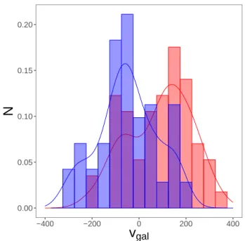
Figure8shows the normalized galactocentric velocity
distri-bution split in negative and positive longitudes where we con-firm the clear signature of the rotation of the nuclear stellar disk
as pointed out bySchönrich et al. (2015). However, due to the
larger sample size now in GALCEN, we noticed a significant
Fig. 7.MDF of the NSC sample ofFeldmeier-Krause et al.(2020)
com-pared to the NSD GALCEN sample confined to |b| < 0.4◦
. 0.00 0.05 0.10 0.15 0.20 −400 −200 0 200 400
v
galN
Fig. 8. Normalized galactocentric velocity distributions for negative longitudes and positive longitudes (in red and blue, respectively) as in
Schönrich et al.(2015). We limited our sample to |l| < 0.5◦
in order to account for the uneven sample distribution.
fraction of high velocity stars exceeding 300 km s−1. These high velocity stars have [Fe/H] > −0.5, ruling out any possible con-nection to the Galactic halo. Do these stars originate from the GC, or could they have been kicked up from a binary supernova explosion, the interaction of a dwarf galaxy or a globular clus-ter with the disk, or inclus-teraction between multiple stars, as
pro-posed byDu et al.(2018)? Proper motion measurements would
be necessary to derive the detailed orbits of those stars in order to understand their origin.
The velocity dispersion of the GALCEN sample is
159 km s−1, with a slightly larger dispersion for the
metal-rich stars (163 km s−1) with respect to the metal-poor stars
(156 km s−1). We define metal rich (MR) and metal poor (MP),
as in Zoccali et al. (2017), as [Fe/H] > 0.1 for MR and
[Fe/H] < −0.1 for MP. Based on GIBS data, while for higher latitudes the MP population shows a larger velocity disper-sion,Zoccali et al.(2017) showed that this trend is inverted by
● ● ● ● ● ● ● ● ● ● ● ● ● ● ● ● ● ● ● ● ● ● ● ● ● ● ● ● ● ● ● ● ● ● ● ● ● ● ● ● ● ● ● ● ● ● ● ● ● ● ● ● ● ● ● ● ● ● ● ● ● ● ● ● ● ● ● ● ● ● ● ● ● ● ● ● ● ● ● ● ● ● ● ● ● ● ● ● ● ● ● ● ● ● ● ● ● ● ● ● ● ● ● ● ● ● ● ● ● ● ● ● ● ● ●● ● ● ● ● ● ● ● ● ● ● ● ● ● ● ● ● ● ● ● ● ● ● ● ● ● ● ● ● ● ● ● ● ● ● ● ● ● ● ● MR, vrot=200 km/s MR, vrot=200 km/s MR, vrot=200 km/s MR, vrot=200 km/s MR, vrot=200 km/s MR, vrot=200 km/s MR, vrot=200 km/s MR, vrot=200 km/s MR, vrot=200 km/s MR, vrot=200 km/s MR, vrot=200 km/s MR, vrot=200 km/s MR, vrot=200 km/s MR, vrot=200 km/s MR, vrot=200 km/s MR, vrot=200 km/s MR, vrot=200 km/s MR, vrot=200 km/s MR, vrot=200 km/s MR, vrot=200 km/s MR, vrot=200 km/s MR, vrot=200 km/s MR, vrot=200 km/s MR, vrot=200 km/s MR, vrot=200 km/s MR, vrot=200 km/s MR, vrot=200 km/s MR, vrot=200 km/s MR, vrot=200 km/s MR, vrot=200 km/s MR, vrot=200 km/s MR, vrot=200 km/s MR, vrot=200 km/s MR, vrot=200 km/s MR, vrot=200 km/s MR, vrot=200 km/s MR, vrot=200 km/s MR, vrot=200 km/s MR, vrot=200 km/s MR, vrot=200 km/s MR, vrot=200 km/s MR, vrot=200 km/s MR, vrot=200 km/s MR, vrot=200 km/s MR, vrot=200 km/s MR, vrot=200 km/s MR, vrot=200 km/s MR, vrot=200 km/s MR, vrot=200 km/s MR, vrot=200 km/s MR, vrot=200 km/s MR, vrot=200 km/s MR, vrot=200 km/s MR, vrot=200 km/s MR, vrot=200 km/s MR, vrot=200 km/s MR, vrot=200 km/s MR, vrot=200 km/s MR, vrot=200 km/s MR, vrot=200 km/s MR, vrot=200 km/s MR, vrot=200 km/s MR, vrot=200 km/s MR, vrot=200 km/s MR, vrot=200 km/s MR, vrot=200 km/s MR, vrot=200 km/s MR, vrot=200 km/s MR, vrot=200 km/s MR, vrot=200 km/s MR, vrot=200 km/s MR, vrot=200 km/s MR, vrot=200 km/s MR, vrot=200 km/s MR, vrot=200 km/s MR, vrot=200 km/s MR, vrot=200 km/s MR, vrot=200 km/s MR, vrot=200 km/s MR, vrot=200 km/s MR, vrot=200 km/s MR, vrot=200 km/s MR, vrot=200 km/s MR, vrot=200 km/s MR, vrot=200 km/s MR, vrot=200 km/s MR, vrot=200 km/s MR, vrot=200 km/s MR, vrot=200 km/s MR, vrot=200 km/s MR, vrot=200 km/s MR, vrot=200 km/s MR, vrot=200 km/s MR, vrot=200 km/s MR, vrot=200 km/s MR, vrot=200 km/s MR, vrot=200 km/s MR, vrot=200 km/s MR, vrot=200 km/s MR, vrot=200 km/s MR, vrot=200 km/s MR, vrot=200 km/s MR, vrot=200 km/s MR, vrot=200 km/s MR, vrot=200 km/s MR, vrot=200 km/s MR, vrot=200 km/s MR, vrot=200 km/s MR, vrot=200 km/s MR, vrot=200 km/s MR, vrot=200 km/s MR, vrot=200 km/s MR, vrot=200 km/s MR, vrot=200 km/s MR, vrot=200 km/s MR, vrot=200 km/s MR, vrot=200 km/s MR, vrot=200 km/s MR, vrot=200 km/s MR, vrot=200 km/s MR, vrot=200 km/s MR, vrot=200 km/s MR, vrot=200 km/s MR, vrot=200 km/s MR, vrot=200 km/s MR, vrot=200 km/s MR, vrot=200 km/s MR, vrot=200 km/s MR, vrot=200 km/s MR, vrot=200 km/s MR, vrot=200 km/s MR, vrot=200 km/s MR, vrot=200 km/s MR, vrot=200 km/s MR, vrot=200 km/s MR, vrot=200 km/s MR, vrot=200 km/s MR, vrot=200 km/s MR, vrot=200 km/s MR, vrot=200 km/s MR, vrot=200 km/s MR, vrot=200 km/s MR, vrot=200 km/s MR, vrot=200 km/s MR, vrot=200 km/s MR, vrot=200 km/s MR, vrot=200 km/s MR, vrot=200 km/s MR, vrot=200 km/s MR, vrot=200 km/s MR, vrot=200 km/s MR, vrot=200 km/s MR, vrot=200 km/s MR, vrot=200 km/s MR, vrot=200 km/s MR, vrot=200 km/s MR, vrot=200 km/s MP, vrot=140 km/s MP, vrot=140 km/s MP, vrot=140 km/s MP, vrot=140 km/s MP, vrot=140 km/s MP, vrot=140 km/s MP, vrot=140 km/s MP, vrot=140 km/s MP, vrot=140 km/s MP, vrot=140 km/s MP, vrot=140 km/s MP, vrot=140 km/s MP, vrot=140 km/s MP, vrot=140 km/s MP, vrot=140 km/s MP, vrot=140 km/s MP, vrot=140 km/s MP, vrot=140 km/s MP, vrot=140 km/s MP, vrot=140 km/s MP, vrot=140 km/s MP, vrot=140 km/s MP, vrot=140 km/s MP, vrot=140 km/s MP, vrot=140 km/s MP, vrot=140 km/s MP, vrot=140 km/s MP, vrot=140 km/s MP, vrot=140 km/s MP, vrot=140 km/s MP, vrot=140 km/s MP, vrot=140 km/s MP, vrot=140 km/s MP, vrot=140 km/s MP, vrot=140 km/s MP, vrot=140 km/s MP, vrot=140 km/s MP, vrot=140 km/s MP, vrot=140 km/s MP, vrot=140 km/s MP, vrot=140 km/s MP, vrot=140 km/s MP, vrot=140 km/s MP, vrot=140 km/s MP, vrot=140 km/s MP, vrot=140 km/s MP, vrot=140 km/s MP, vrot=140 km/s MP, vrot=140 km/s MP, vrot=140 km/s MP, vrot=140 km/s MP, vrot=140 km/s MP, vrot=140 km/s MP, vrot=140 km/s MP, vrot=140 km/s MP, vrot=140 km/s MP, vrot=140 km/s MP, vrot=140 km/s MP, vrot=140 km/s MP, vrot=140 km/s MP, vrot=140 km/s MP, vrot=140 km/s MP, vrot=140 km/s MP, vrot=140 km/s MP, vrot=140 km/s MP, vrot=140 km/s MP, vrot=140 km/s MP, vrot=140 km/s MP, vrot=140 km/s MP, vrot=140 km/s MP, vrot=140 km/s MP, vrot=140 km/s MP, vrot=140 km/s MP, vrot=140 km/s MP, vrot=140 km/s MP, vrot=140 km/s MP, vrot=140 km/s MP, vrot=140 km/s MP, vrot=140 km/s MP, vrot=140 km/s MP, vrot=140 km/s MP, vrot=140 km/s MP, vrot=140 km/s MP, vrot=140 km/s MP, vrot=140 km/s MP, vrot=140 km/s MP, vrot=140 km/s MP, vrot=140 km/s MP, vrot=140 km/s MP, vrot=140 km/s MP, vrot=140 km/s MP, vrot=140 km/s MP, vrot=140 km/s MP, vrot=140 km/s MP, vrot=140 km/s MP, vrot=140 km/s MP, vrot=140 km/s MP, vrot=140 km/s MP, vrot=140 km/s MP, vrot=140 km/s MP, vrot=140 km/s MP, vrot=140 km/s MP, vrot=140 km/s MP, vrot=140 km/s MP, vrot=140 km/s MP, vrot=140 km/s MP, vrot=140 km/s MP, vrot=140 km/s MP, vrot=140 km/s MP, vrot=140 km/s MP, vrot=140 km/s MP, vrot=140 km/s MP, vrot=140 km/s MP, vrot=140 km/s MP, vrot=140 km/s MP, vrot=140 km/s MP, vrot=140 km/s MP, vrot=140 km/s MP, vrot=140 km/s MP, vrot=140 km/s MP, vrot=140 km/s MP, vrot=140 km/s MP, vrot=140 km/s MP, vrot=140 km/s MP, vrot=140 km/s MP, vrot=140 km/s MP, vrot=140 km/s MP, vrot=140 km/s MP, vrot=140 km/s MP, vrot=140 km/s MP, vrot=140 km/s MP, vrot=140 km/s MP, vrot=140 km/s MP, vrot=140 km/s MP, vrot=140 km/s MP, vrot=140 km/s MP, vrot=140 km/s MP, vrot=140 km/s MP, vrot=140 km/s MP, vrot=140 km/s MP, vrot=140 km/s MP, vrot=140 km/s MP, vrot=140 km/s MP, vrot=140 km/s MP, vrot=140 km/s MP, vrot=140 km/s MP, vrot=140 km/s MP, vrot=140 km/s MP, vrot=140 km/s MP, vrot=140 km/s MP, vrot=140 km/s MP, vrot=140 km/s MP, vrot=140 km/s MP, vrot=140 km/s MP, vrot=140 km/s MP, vrot=140 km/s MP, vrot=140 km/s ● ● ● ● ● ● ● ● ● ● ● ● ● ● ● ● ● ● ● ● ● ● ● ● ● ● ● ● ● ● ● ● ● ● ● ● ● ● ● ● ● ● ● ● ● ● ● ● ● ● ● ● ● ● ● ● ● ● ● ● ● ● ● ● ● ● ● ● ● ● ● ● ● ● ● ● ● ● ● ● ● ● ● ● ● ● ● ● ● ● ● ● ● ● ● ● ● ● ● ● ● ● ● ● ● ● ● ● ● ● ● ● ● ● ● ● ● ● ● ● ● ● ● ● ● ● ● ● ● ● ● ● ● ● ● ● ● ● ● ● ● ● ● ● ● ● ● ● ● ● ● ● ● ● ● ● ● ● ● ● ● ● ● ● ● ● ● ● ● ● ● ● ● ● ● ● ● ● ● ● ● ● ● ● ● ● ● ● ● ● ● ● ● ● ● ● ● ● ● ● ● ● ● ●|b| < 0.5|b| < 0.5|b| < 0.5|b| < 0.5|b| < 0.5|b| < 0.5|b| < 0.5|b| < 0.5|b| < 0.5|b| < 0.5|b| < 0.5|b| < 0.5|b| < 0.5|b| < 0.5|b| < 0.5|b| < 0.5|b| < 0.5|b| < 0.5|b| < 0.5|b| < 0.5|b| < 0.5|b| < 0.5|b| < 0.5|b| < 0.5|b| < 0.5|b| < 0.5|b| < 0.5|b| < 0.5|b| < 0.5|b| < 0.5|b| < 0.5|b| < 0.5|b| < 0.5|b| < 0.5|b| < 0.5|b| < 0.5|b| < 0.5|b| < 0.5|b| < 0.5|b| < 0.5|b| < 0.5|b| < 0.5|b| < 0.5|b| < 0.5|b| < 0.5|b| < 0.5|b| < 0.5|b| < 0.5|b| < 0.5|b| < 0.5|b| < 0.5|b| < 0.5|b| < 0.5|b| < 0.5|b| < 0.5|b| < 0.5|b| < 0.5|b| < 0.5|b| < 0.5|b| < 0.5|b| < 0.5|b| < 0.5|b| < 0.5|b| < 0.5|b| < 0.5|b| < 0.5|b| < 0.5|b| < 0.5|b| < 0.5|b| < 0.5|b| < 0.5|b| < 0.5|b| < 0.5|b| < 0.5|b| < 0.5|b| < 0.5|b| < 0.5|b| < 0.5|b| < 0.5|b| < 0.5|b| < 0.5|b| < 0.5|b| < 0.5|b| < 0.5|b| < 0.5|b| < 0.5|b| < 0.5|b| < 0.5|b| < 0.5|b| < 0.5|b| < 0.5|b| < 0.5|b| < 0.5|b| < 0.5|b| < 0.5|b| < 0.5|b| < 0.5|b| < 0.5|b| < 0.5|b| < 0.5|b| < 0.5|b| < 0.5|b| < 0.5|b| < 0.5|b| < 0.5|b| < 0.5|b| < 0.5|b| < 0.5|b| < 0.5|b| < 0.5|b| < 0.5|b| < 0.5|b| < 0.5|b| < 0.5|b| < 0.5|b| < 0.5|b| < 0.5|b| < 0.5|b| < 0.5|b| < 0.5|b| < 0.5|b| < 0.5|b| < 0.5|b| < 0.5|b| < 0.5|b| < 0.5|b| < 0.5|b| < 0.5|b| < 0.5|b| < 0.5|b| < 0.5|b| < 0.5|b| < 0.5|b| < 0.5|b| < 0.5|b| < 0.5|b| < 0.5|b| < 0.5|b| < 0.5|b| < 0.5|b| < 0.5|b| < 0.5|b| < 0.5|b| < 0.5|b| < 0.5|b| < 0.5|b| < 0.5|b| < 0.5|b| < 0.5|b| < 0.5|b| < 0.5|b| < 0.5|b| < 0.5|b| < 0.5|b| < 0.5|b| < 0.5|b| < 0.5 −400 −200 0 200 400 −1.0 −0.5 0.0 0.5 1.0
l
V
GC
Fig. 9.Galactocentric radial velocity vs. galactic longitude. The black line shows the linear fit of the full GALCEN sample, while the red line shows the fit for metal-rich stars [Fe/H] > 0, and the blue line shows MP stars. The shaded area shows the 95% level of confidence interval. The green points are stars inside 0.4 degrees of galactic latitude. See text for details.
proper motion measurements,Clarkson et al.(2018) found that
the metal-rich population shows a steeper rotation curve. Our analysis of GALCEN confirms their results with an increasing velocity dispersion with higher metallicity.Kunder et al.(2016) showed that metal-poor stars such as RR Lyrae rotate much more slowly than RGB or RC stars in the bulge, and they sug-gested that they belong to the classical bulge. Other studies also reveal the presence of an old population in the GC region
(see e.g., Contreras Ramos et al. 2018, Dong et al. 2017, and
Minniti et al. 2016). Based on the GIBS RC stars,Zoccali et al.
(2017) gave some indications that MP stars show a marginally
slower rotation compared to the MR stars (see their Fig. 13). We investigated this in more detail by tracing the slope of the MR and MP stars in the l vs. vGCplane. We used a similar method for
the fitting procedure toSchönrich et al.(2015). Figure9shows a linear fit of the entire GALCEN sample (black line) as well as the fit for the MR stars (red solid line) and MP stars (blue solid line). The rotational speed can be calculated by assuming
a radius for the NSD as shown by Eq. (2), assuming a typical
radius R of the NSD of 120 pc:
vrad= R0× sin(l) × (V/RNSD− V0/R0), (2)
where vrad is the heliocentric radial velocity, R0 = 8.2 kpc
(dis-tance to the GC), V0 = 220 km s−1(sun velocity), l the galactic
longitude, and RNSDthe radius of the disk (120 pc).
For the best fit (indicated by the blue and red line for both the MP and MR population, respectively), we obtain a rotation velocity of 140 ± 30 km s−1for the MP stars and 200 ± 30 km s−1
for the MR stars, clearly indicating a faster rotation for the
MR stars. If we restrict our sample to |b| ≤ 0.4◦, which is
the approximate vertical extent of the nuclear stellar disk (see
Fig. 2), we obtain very similar fitting results. The reason for
this difference in the rotation velocity between MR and MP
stars may have a different origin. For example, MP stars could
be formed from disrupted stellar clusters. Tsatsi et al. (2017)
showed that using N-body simulation of inspiralling clusters to the center of the Milky Way can reproduce both the morpholog-ical and kinematmorpholog-ical properties of the NSC. On the other hand,
Mastrobuono-Battisti et al. (2019) showed that in the presence of an aspherical, time-variable potential (e.g., due to the pres-ence of a discrete stellar black hole cusp), counter-rotating disks can perturb the dynamics of older stellar populations leading to accelerated relaxation, while the younger populations show a larger amount of rotation. Younger populations always show larger rotation compared to older ones, but the difference is even larger for counter-rotating disks. Age information and chemical footprints such as dispersion in light elements (Schiavon et al. 2017) would be essential to understand the different possible for-mation scenarios.
8. Conclusions
Using the latest DR16 APOGEE data release, we studied cool M giants in the GALCEN sample going down to tempera-tures of 3200 K. Among those, stellar parameters of a bunch
of known and candidate AGB/supergiant stars are now
avail-able thanks to the cool grid of MARCS model atmospheres and significant improvements in the analysis of cool stars by
the APOGEE/ASPCAP team. The known (6) and candidate
(15) AGB/supergiant stars are situated well above the tip of the RGB, confirming their status as cool luminous stars. We con-firm that a photometric H–K color cut combined with a dered-dened magnitude cut of K0is a very powerful criterion to select
AGB/supergiant stars. In the MDF of GALCEN, we clearly
iden-tify a metal-poor peak at [Fe/H] = −0.53 dex, which is about
0.2 dex lower than the metal-poor peak in BW. About 50% of the stars belong to each of the MR and MP populations. The group
of AGB/supergiant stars follows the same trend in the MDF as
the normal M giants. The general α-abundances of the GAL-CEN stars show a very bulge-like behavior. As already pointed out by Schönrich et al. (2015), we identify the rotation of the nuclear disk seen in the galactic longitude vs. vGCdiagram.
Sep-arating our sample in an MR and MP population, we detect a
much higher rotation velocity of the MR stars with 200 km s−1
with respect to the MP stars (140 km s−1), indicating a different
origin of these two populations. We see evidence of clear dif-ferences in the chemical footprints of the nuclear disk and the NSCs, both in chemical abundances and the MDF. Together with
their different SFH, it is likely that the NSD and the NSC have
formed on different time scales.
Acknowledgements. We want to thank the anonymous referee for her/his very fruitful and valuable comments. MS thanks A. Mastrobueno-Battisti for very fruitful discussions. We want to thank Anja Feldmeier-Krause to make their table of metallicities for the NSC available. M. S. acknowledges the Programme National de Cosmologie et Galaxies (PNCG) of CNRS/INSU, France, for financial support. DM is supported by the BASAL Center for Astrophysics and Associated Technologies (CATA) through Grant AFB 170002, by the Programa Iniciativa Científica Milenio grant IC120009, awarded to the Mil-lennium Institute of Astrophysics (MAS), and by Project FONDECYT No. 1170121. DAGH and O. Z. acknowledge support from the State Research Agency (AEI) of the Spanish Ministry of Science, Innovation and Universi-ties (MCIU) and the European Regional Development Fund (FEDER) under grant AYA2017-88254-P. J. G. F.-T. is supported by FONDECYT No. 3180210 and Becas Iberoamérica Investigador 2019, Banco Santander Chile. S. H. is supported by an NSF Astronomy and Astrophysics Postdoctoral Fellowship under award AST-1801940. R. R. M. acknowledges partial support from project BASAL AFB-170002 as well as FONDECYT project N◦1170364. Funding for
SDSS-III has been provided by the Alfred P. Sloan Foundation, the Partici-pating Institutions, the National Science Foundation, and the US Department of Energy Office of Science. The SDSS-III web site ishttp://www.sdss3. org/. SDSS-III is managed by the Astrophysical Research Consortium for the


![Fig. 9. Galactocentric radial velocity vs. galactic longitude. The black line shows the linear fit of the full GALCEN sample, while the red line shows the fit for metal-rich stars [Fe/H] > 0, and the blue line shows MP stars](https://thumb-eu.123doks.com/thumbv2/123doknet/13326089.400383/10.892.74.423.121.465/galactocentric-radial-velocity-galactic-longitude-linear-galcen-sample.webp)