HAL Id: hal-00379329
https://hal.archives-ouvertes.fr/hal-00379329v2
Submitted on 27 Oct 2010
HAL is a multi-disciplinary open access
archive for the deposit and dissemination of
sci-entific research documents, whether they are
pub-lished or not. The documents may come from
teaching and research institutions in France or
abroad, or from public or private research centers.
L’archive ouverte pluridisciplinaire HAL, est
destinée au dépôt et à la diffusion de documents
scientifiques de niveau recherche, publiés ou non,
émanant des établissements d’enseignement et de
recherche français ou étrangers, des laboratoires
publics ou privés.
Image restoration using a kNN-variant of the mean-shift
Cesario Vincenzo Angelino, Eric Debreuve, Michel Barlaud
To cite this version:
Cesario Vincenzo Angelino, Eric Debreuve, Michel Barlaud. Image restoration using a kNN-variant of
the mean-shift. IEEE International Conference on Image Processing, Oct 2008, San Diego, California,
United States. �hal-00379329v2�
IMAGE RESTORATION USING A KNN-VARIANT OF THE MEAN-SHIFT
Cesario Vincenzo Angelino, Eric Debreuve, Michel Barlaud
Laboratory I3S, University of Nice-Sophia Antipolis/CNRS, France
ABSTRACT
The image restoration problem is addressed in the variational framework. The focus was set on denoising. The statistics of natural images are consistent with the Markov random field principles. Therefore, a restoration process should preserve the correlation between adjacent pixels. The proposed ap-proach minimizes the conditional entropy of a pixel knowing its neighborhood. The conditional aspect helps preserving lo-cal image structures such as edges and textures. The statistilo-cal properties of the degraded image are estimated using a novel, adaptive weighted k-th nearest neighbor (kNN) strategy. The derived gradient descent procedure is mainly based on mean-shift computations in this framework.
Index Terms— Image restoration, joint conditional
en-tropy, k-th nearest neighbors, mean-shift
1. INTRODUCTION
The goal of image restoration is to recover an image that has been degraded by some stochastic process. Research focus was set on removing additive, independent, random noise, however more general degradations phenomenons can be modeled, such as blurring, non-independent noise, and so on. The literature of image restoration is vast and methods have been proposed in frameworks such as linear and non-linear filtering in either the spatial domain or transformed domains. Nonlinear filtering approaches typically lead to algorithms based on partial differential equations, e.g. in the variational framework [1]. However, these methods rely on local, weighted clique-like constraints. In other words, these constraints apply within pixel neighborhoods. Even if they are designed to preserve edges, the imposed coherence be-tween the pixels of a neighborhood inevitably results in some smoothness within image patches. On the opposite, nonlo-cal methods make use of long range, high order coherences to infer (statistical) properties of the degraded image and perform an adaptively constrained restoration [2, 3]. These approaches are supported by studies on the statistics and topology of spaces of natural images [4, 5] which confirm that patches of natural images tends to fill space unevenly, forming manifolds of lower dimensions. Such subspaces correspond to correlations that exist not within patches but between patches and that should be take into account in a
restoration process in order to preserve the image structures. In this context, the idea is to consider the intensity or color of a pixel jointly with, or conditionally with respect to, the intensities or colors of its neighbors. An interesting approach for denoising consists in minimizing the conditional entropy of a pixel intensity or color knowing its neighborhood [2].
In this paper, the same philosophy is followed while a number of theoretical and practical obstacles encountered in [2] are naturally overcome using a novel adaptive strat-egy in the k-th nearest neighbor (kNN) framework. These obstacles are mostly due to the use of Parzen windowing to estimate the joint probability density function (PDF), (i) esti-mation which is stated to be required in [2].
(ii) As acknowledged by the authors, the high-dimensional
and scattered nature of the samples (the N ×N -image patches seen as N2-vectors) requires to use a wide Parzen window,
which oversmoothes the PDF and, consequently, biases the entropy estimation.
The difficulties (i) and (ii) disappear in the kNN framework since entropy can be estimated directly from the samples (i.e., without explicit PDF estimation) in a simple manner which naturally accounts for the local sample density.
2. NEIGHBORHOOD CONSTRAINED DENOISING Let us model an image as a random field X. Let T be the set of pixels of the image and Ntbe a neighborhood of pixel
t ∈ T . We define a random vector Y (t) = {X(t)}t∈Nt,
corresponding to the set of intensities at the neighbors of pixel
t. We also define a random vector Z(t) = (X(t), Y (t)) to
denote image regions or patches, i.e., pixels combined with their neighborhoods.
Image restoration is an inverse problem, that can be formulated as a functional minimization problem. As dis-cussed in section 1, natural images exhibit correlation be-tween patches, thus we consider the conditional entropy functional, i.e., the uncertainty of the random pixel X when its neighborhood is given, as suitable measure for denoising applications.
Indeed, when noise is added, some of the information car-ried by the neighborhood is lost, so the uncertainty of a pixel knowing its neighborhood is greater in the average. This is formally stated by the following proposition:
Proposition 1. Let X be a random variable and Y a random
vector representing its neighborhood. Let ˜X be the sum of X with a white gaussian noise N independent from X. Let ˜Y be the neighborhood vector constructed from ˜X. Then
h( ˜X| ˜Y ) ≥ h(X|Y ). (1)
Proof. By definition we have h( ˜X| ˜Y ) = h( ˜X) − I( ˜X; ˜Y )
and h(X|Y ) = h(X) − I(X; Y ) where I(·; ·) denote the mu-tual information. First note that h( ˜X) is greater than h(X)
since the addition of two independent random variables in-creases the entropy [6]. X → Y → ˜Y forms a Markov chain,
since ˜Y and X are conditionally independent given Y . Thus,
the data processing inequality [6] reads
I(X; Y ) ≥ I(X; ˜Y ). (2) Since ˜Y → X → ˜X forms a Markov chain itself (since the
noise is white and gaussian), than we obtain
I( ˜Y ; X) ≥ I( ˜Y ; ˜X). (3) By combining Eq. (2) and Eq. (3) we have I(X; Y ) ≥
I( ˜X; ˜Y ).
Proposition 1 gives information theoretic basis for mini-mize the conditional entropy. Thus, the recovered image ide-ally satisfies
X∗= arg min
X h(X|Y = yi) (4)
Entropy functional can be approximated by the Ahmad-Lin estimator [7] h(X|Y = yi) ≈ − 1 |T | X tj∈T log p(xj|yi), (5) where p(s|yi) = 1 |Tyi| X tm∈Tyi K(s − xm), (6)
is the kernel estimate of the PDF, with the symmetric kernel
K(·). The set Tyi in Eq. (6) is the set of index pixels which
have the same neighborhood yi. In order to solve the opti-mization problem (4) a steepest descent algorithm is used. It can be shown that the energy derivative of (5) is
∂h(X|Y = yi) ∂xi = − 1 |T | ∇p(zi) p(zi) ∂zi ∂xi + χ(xi), (7) with χ(xi) = 1 |T | 1 |Tyi| X tj∈T ∇K(xj− xi) p(xj|yi) . (8) The term χ(·) of Eq. (8) is difficult to estimate, however if the kernel K(·) has a narrow window size, only sample very close to the actual estimation point will contribute to the pdf. Un-der this assumption the conditional pdf is p(s|yi) ≈ Ns/|Tyi|,
where Nsis the number of pixels equal to s. Thus by substi-tuting and observing that ∇K(·) is an odd function, we ob-serve that χ(xi) is negligible for almost every value assumed by xi. In the following we will not consider this term. Thus the energy derivative is a mean-shift [8] term on the high di-mensional joint pdf of Z, multiplied by a projection term.
Density estimation requires the sample sequence {Xi}i∈N to be drawn from the same distribution, i.e., it requires the stationarity of the signal. As it is well-known, image signals are piecewise stationary, thus closer pixel are supposed to better represent the distribution of the current pixel. As a consequence, we ’apply’ a label to the actual sample patch
Ziby adding to its N2-vector representation the spatial coor-dinates of its center, i.e., the coorcoor-dinates of the current pixel
xi. Formally, the PDF of Z(t), t ∈ T , is replaced with the PDF of {Z(t), t}, t ∈ T . For simplicity, in the following we denote with Z the (N2+ 2)-dimensional vector of this
augmented feature space.
3. MEAN SHIFT ESTIMATION
In order to minimize the energy (4) via a steepest descent al-gorithm, the term (7), has to be estimated. Since no assump-tions are made on the underlying PDF, we rely on nonpara-metric techniques to obtain density estimates, in particular we refer to kernel estimation.
In the multi-dimensional density estimation literature a lot of estimators have been proposed. These estimators can be classified on the behavior of the kernel size h. In particular,
(i) Parzen Estimator: it is the most popular and simple kernel
estimator in which h is constant,and (ii) Balloon Estimator: the kernel size depends on the estimation point z. The kNN estimator [8] is a particular case of balloon estimator. 3.1. Parzen Method and its limitations
The Parzen method makes no assumption about the actual PDF and is therefore qualified as nonparametric. The mean-shift in the Parzen Window approach can be expressed, using an Epanechnikov kernel, as [8] ∇p(zi) p(zi) = d + 2 h2 1 k(zi, h) X zj∈Sh(zi) (zj− zi), (9)
where d is the dimension of Z, Sh(zi) is the support of the Parzen kernel centered at point zi and of size h, k being the number of observation falling into Sh(X). The choice of the kernel window size h is critical [9]. If h is too large, the es-timate will suffer from too little resolution, otherwise if h is too small, the estimate will suffer from too much statistical variability.
As the dimension of the data space increases, the space sam-pling gets sparser (problem known as the curse of dimension-ality). Therefore, less samples fall into the Parzen window
0 20 40 60 80 100 5 10 15 20 25
Number of Nearest Neighbors (NNs)
RMSE σ = 5 σ = 10 σ = 15 σ = 20 σ = 25
Fig. 1. RMSE in function of the numbers of nearest neighbors for different levels of noise.
centered on each sample, making the PDF estimation less re-liable. Dilating the Parzen window does not solve this prob-lem since it leads to over-smoothing the PDF. This is due to the fixed window size: the method cannot adapt to the local sample density.
3.2. kNN Framework and adaptive weighting
In the Parzen-window approach, the PDF at sample s is re-lated to the number of samples falling into a window of fixed size centered on the sample. The kNN method is the dual approach: the density is related to the size of the window necessary to include the k nearest neighbors of the sample. Thus, this estimator tries to incorporate larger bandwidths in the tails of the distributions, where data are scarce. The choice of k appears to be much less critical than the choice of h in the Parzen method [10]. In kNN framework, the mean-shift vector is given by [8] ∇p(zi) p(zi) = d + 2 ρ2 k 1 k X zj∈Sρk zj− zi, (10)
where ρk is the distance to the k-th nearest neighbor. The integral of the kNN PDF estimator is not equal to one (hence, the kernel is not a density) and the discontinuous nature of the bandwidth function manifests directly into discontinuities in the resulting estimate. Furthermore, the estimator has severe bias problems, particularly in the tails [11] although it seems to perform well in higher dimension [12].
However, as near the distribution modes there is an high density of samples, the window size associate to the k-th nearest neighbor could be too small. In this case the estimate will be sensible to the statistical variation in the distribution. To avoid this problem we would increase the number of near-est neighbors, to have an appropriate window size near the modes. However this choice would produce a window too large in the tails of the distribution. Thus very far samples would contribute to the estimation, producing severe bias problems.
We propose, as an alternative solution, to weight the contribution of the samples. Intuitively, the weights must be a function of distance between the actual sample and the
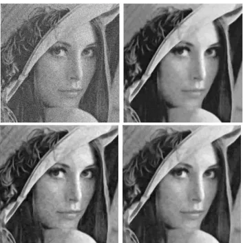
Fig. 2. Comparison of restored images. (In lexicographic order) Noisy image, UINTA restored, kNN restored (k = 10) and kNN restored (k = 40).
ith nearest neighbor, i.e., samples with smaller distance are
weighted more heavily than ones with larger distance
wj = exp − 1 2α2 0 µ ρj ρmax k ¶2 (11)
where α0represents the ’effective’ kernel shape in the lowest
density location, i.e., when ρk(zj) = ρmax
k . This adaptive weighted kNN (AWkNN) approach solves the bias problem of the kNN estimator. In this case the mean shift term is replaced by ∇p(zi) p(zi) = d + 2 ρ2 k 1 Pk j=1wj X zj∈Sρk wj(zj− zi). (12)
4. ALGORITHM AND EXPERIMENTAL RESULTS The method proposed minimizes the conditional entropy (5) using a gradient descent. The derivative (7) is estimated in the adaptive weighted kNN framework, as explained in sec-tion 3.2. In this case the term ∇p/p is expressed by Eq. (12). Thus the steepest descent algorithm is performed with the fol-lowing evolution equation
x(n+1)i = x(n)i − νd + 2 ρ2 k X zj∈Sρk ¯ wj(zj− zi)∂zi ∂xi, (13)
where ν is the step size and ¯wjare the weight coefficients of Eq. (11), normalized to have sum equal to 1.
At each iteration the mean-shift vector (12) in the high di-mensional space Z is calculated. The high didi-mensional space
is given by considering jointly the intensity of the current pixel and that of its neighborhood, and by adding the two spatial features as explained in section 2. The pixel value xi is then updated by means of Eq. (13).
The k nearest neighbors are provided by the Approximate Nearest Neighbor Searching (ANN) library (available at
http://www.cs.umd.edu/˜mount/ANN/).
In order to measure the performance of our algorithm we degraded the Lena image (256x256) adding a gaussian noise with standard deviation σ = 10. The original image has in-tensity ranging from 0 to 100. We consider a 9 x 9 neighbor-hoods, and we add spatial features to the original radiometric data [10, 13], as explained in section 2. These spatial features allow us to reduce the effect of the non stationarity of the sig-nal in the estimation process, by preferring regions closer to the estimation point. The dimension of the data d is therefore equal to 83, and we have to search the k nearest neighbors in such a high dimensional space.
Figure 2 shows a comparison of the restored images. Fig-ure 1 shows the Root Mean Square Error (RMSE) curves in function of the number of nearest neighbors k for different levels of noise. Varying the parameter k within a signifi-cant range does not provide any signifisignifi-cant changes in the results. In Table 1, the optimal values of the RMSE and the Structure SIMilarity Index (SSIM) [14] are shown. On this experiment our algorithm provides results comparable with or slightly better than UINTA when k ∈ [10; 50]. In terms of speed, our algorithm is much faster than UINTA, due to the AWkNN framework. Indeed, UINTA have to update the Parzen window size at each iteration. To do this a time con-suming cross validation optimization is performed. On the contrary our method simply adapts the PDF changes during the minimization process. For instance, the cpu time with Matlab for the UINTA algorithm is almost 4500 sec. Our al-gorithm, with k = 10, takes only 600 sec. We did some more experiments on Lena with different noise levels (see Table 2).
RMSE SSIM RMSE SSIM
k=3 5.51 0.918 UINTA 4.65 0.890
k=10 4.01 0.910 k=40 4.50 0.889
k=20 4.14 0.905 k=50 4.64 0.882
k=30 4.35 0.895 k=100 5.12 0.832
Table 1. RMSE and SSIM values for different values of k, and for UINTA.
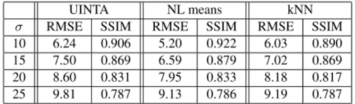
UINTA NL means kNN
σ RMSE SSIM RMSE SSIM RMSE SSIM
10 6.24 0.906 5.20 0.922 6.03 0.890
15 7.50 0.869 6.59 0.879 7.02 0.869
20 8.60 0.831 7.95 0.833 8.18 0.817
25 9.81 0.787 9.13 0.786 9.19 0.787
Table 2. Comparison between UINTA, Non Local Means [3], and the proposed method for different noise levels on Lena. Each result was obtained with the optimal parameters for the corresponding algorithm.
5. CONCLUSION
This paper presented a restoration method in the variational framework based on the minimization of the conditional entropy using the kNN framework. In particular a novel, AWkNN strategy, which solve the bias problems of kNN estimators, has been proposed. The simulations indicated slightly better results in RMSE and SSIM measures with respect to the UINTA algorithm and a marked gain in cpu speed. Results are even more promising considering that no regularization is applied.
As future work, the method could be regularized. In terms of application, a similar approach could apply to image in-painting.
6. REFERENCES
[1] Leonid I. Rudin, Stanley Osher, and Emad Fatemi, “Nonlinear total variation based noise removal algorithms,” Phys. D, vol. 60, no. 1-4, pp. 259–268, 1992.
[2] Suyash P. Awate and Ross T. Whitaker, “Unsupervised,
information-theoretic, adaptive image filtering for image restoration,” IEEE Trans. Pattern Anal., vol. 28, no. 3, pp. 364–376, 2006.
[3] Antoni Buades, Bartomeu Coll, and Jean-Michel Morel, “A non-local algorithm for image denoising,” in CVPR, Washing-ton, DC, USA, 2005.
[4] G. Carlsson, T. Ishkhanov, V. de Silva, and A. Zomorodian, “On the local behavior of spaces of natural images,” Int. J.
Comput. Vision, vol. 76, no. 1, pp. 1–12, 2008.
[5] J. Huang and D. Mumford, “Statistics of natural images and models,” in CVPR, Ft. Collins, CO, USA, 1999.
[6] T. Cover and J. Thomas, Elements of Information Theory, Wiley-Interscience, first edition, 1991.
[7] I. A. Ahmad and P. Lin, “A nonparametric estimation of the entropy for absolutely continuous distributions,” IEEE Trans.
Inform. Theory, vol. 22, pp. 372–375, 1976.
[8] K. Fukunaga and L. D. Hostetler, “The estimation of the gra-dient of a density function, with applications in pattern recog-nition,” IEEE Trans. Inform. Theory, vol. 21, no. 1, pp. 32–40, 1975.
[9] D. Scott, Multivariate Density Estimation: Theory, Practice,
and Visualization, Wiley, second edition, 1992.
[10] S. Boltz, E. Debreuve, and M. Barlaud, “High-dimensional statistical distance for region-of-interest tracking: Application to combining a soft geometric constraint with radiometry,” in
CVPR, Minneapolis, USA, 2007.
[11] Y. Mack and M. Rosenblatt, “Multivariate k-nearest neighbor density estimates,” Journal of Multivariate Analysis, vol. 9, pp. 1–15, 1979.
[12] G.R. Terrell and D.W. Scott, “Variable kernel density estima-tion,” Annals of Statistics, vol. 20, pp. 1236–1265, 1992. [13] A. Elgammal, R. Duraiswami, and L. S. Davis, “Probabilistic
tracking in joint feature-spatial spaces,” in CVPR, Madison, WI, 2003.
[14] Z. Wang, A. C. Bovik, H. R. Sheikh, and E. P. Simoncelli, “Image quality assessment: From error visibility to structural similarity,” IEEE Trans. Image Process., vol. 13, no. 4, pp. 600–612, 2004.