Bayesian Calibration of the Mg/Ca Paleothermometer in Planktic Foraminifera

HAL Id: hal-02973694

https://hal.archives-ouvertes.fr/hal-02973694

Submitted on 28 Oct 2020

HAL is a multi-disciplinary open access

archive for the deposit and dissemination of

sci-entific research documents, whether they are

pub-lished or not. The documents may come from

teaching and research institutions in France or

abroad, or from public or private research centers.

L’archive ouverte pluridisciplinaire HAL, est

destinée au dépôt et à la diffusion de documents

scientifiques de niveau recherche, publiés ou non,

émanant des établissements d’enseignement et de

recherche français ou étrangers, des laboratoires

publics ou privés.

Jessica E. Tierney, Steven B. Malevich, William Gray, Lael Vetter, Kaustubh

Thirumalai

To cite this version:

Jessica E. Tierney, Steven B. Malevich, William Gray, Lael Vetter, Kaustubh Thirumalai. Bayesian

Calibration of the Mg/Ca Paleothermometer in Planktic Foraminifera. Paleoceanography and

Pale-oclimatology, American Geophysical Union, 2019, 34 (12), pp.2005-2030. �10.1029/2019PA003744�.

�hal-02973694�

Jessica E. Tierney1 _{, Steven B. Malevich}1 _{, William Gray}2 _{, Lael Vetter}1_,

and Kaustubh Thirumalai1

1_{Department of Geosciences, University of Arizona, Tucson, AZ, USA,}2_{Laboratoire des Sciences du Climat et de} l'Environnement (LSCE/IPSL), Gif-sur-Yvette, France

Abstract

The Mg/Ca ratio of planktic foraminifera is a widely used proxy for sea-surface temperature but is also sensitive to other environmental factors. Previous work has relied on correcting Mg/Ca for nonthermal influences. Here, we develop a set of Bayesian models for Mg/Ca in four major planktic groups—Globigerinoides ruber (including both pink and white chromotypes), Trilobatus sacculifer,

Globigerina bulloides, and Neogloboquadrina pachyderma (including N. incompta)—that account for the multivariate influences on this proxy in an integrated framework. We use a hierarchical model design that leverages information from both laboratory culture studies and globally distributed core top data, allowing us to include environmental sensitivities that are poorly constrained by core top observations alone. For applications over longer geological timescales, we develop a version of the model that incorporates changes in the Mg/Ca ratio of seawater. We test our models—collectively referred to as BAYMAG—on sediment trap data and on representative paleoclimate time series and demonstrate good agreement with observations and independent sea-surface temperature proxies. BAYMAG provides probabilistic estimates of past temperatures that can accommodate uncertainties in other environmental influences, enhancing our ability to interpret signals encoded in Mg/Ca.

Plain Language Summary

The amount of magnesium (Mg) incorporated into the calcite shells of tiny protists called foraminifera is determined by the temperature of the water in which they grew. This allows paleoclimatologists to measure the magnesium-to-calcium (Mg/Ca) ratio of fossil foraminiferal shells and determine how past sea-surface temperatures have changed. However, other factors can influence Mg/Ca, like the salinity and pH of seawater. Here, we develop Bayesian models of foraminiferal Mg/Ca that account for all of the influences on Mg/Ca and show how we can use these to improve our interpretations of Mg/Ca data.

1. Introduction

The magnesium-to-calcium (Mg/Ca) ratio of planktic foraminifera is a commonly used proxy method for reconstructing past sea-surface temperatures (SSTs). It has played a pivotal role informing our understand-ing of tropical climate dynamics in the Late Quaternary (Lea et al., 2000, 2003; Rosenthal et al., 2003; Stott et al., 2007) as well as in deeper geologic time (e.g., Evans et al., 2018). The proxy has theoretical basis in thermodynamics, which predicts a nonlinear increase in Mg incorporation into calcite as temperatures rise (Oomori et al., 1987). Laboratory culturing of planktic foraminifera confirms an exponential dependence of Mg/Ca on temperature, albeit with a stronger sensitivity than thermodynamic predictions, indicating that biological “vital effects” also play a role (Lea et al., 1999; Nürnberg et al., 1996). Laboratory experiments also demonstrate that Mg/Ca in foraminifera is sensitive to other environmental factors, such as salinity and pH (Evans, Wade, et al., 2016; Dueñas-Bohórquez et al., 2009; Hönisch et al., 2013; Kisakürek et al., 2008; Lea et al., 1999). The extent to which these secondary factors compromise SST prediction from Mg/Ca is an ongoing topic of investigation (Arbuszewski et al., 2010; Evans, Wade, et al., 2016; Ferguson et al., 2008; Gray & Evans, 2019; Gray et al., 2018; Hönisch et al., 2013; Mathien-Blard & Bassinot, 2009). Beyond com-peting environmental factors, the depositional environment also influences Mg/Ca. If the calcite saturation state of the bottom waters is low, partial dissolution of foraminiferal calcite occurs, lowering Mg/Ca (Brown & Elderfield, 1996; Regenberg et al., 2006, 2014; Rosenthal et al., 2000).

Key Points:

• We introduce Mg/Ca Bayesian calibrations for planktic foraminifera • Hierarchical modeling is used

to constrain multivariate Mg/Ca sensitivities

• For deep-time applications, we incorporate estimates of Mg/Ca of seawater Supporting Information: • Supporting Information S1 • Data Set S1 • Data Set S2 • Data Set S3 • Data Set S4 • Data Set S5 Correspondence to: J. E. Tierney, jesst@email.arizona.edu Citation:

Tierney, J. E., Malevich, S. B., Gray, W., Vetter, L., & Thirumalai, K. (2019). Bayesian calibration of the Mg/Ca paleothermometer in planktic foraminifera. Paleoceanography and Paleoclimatology,

https://doi. org/10.1029/2019PA003744

Received 1 AUG 2019 Accepted 31 OCT 2019

Accepted article online 12 NOV 2019

©2019. American Geophysical Union. All Rights Reserved.

Published online 13 DEC 2019

2005 2030.– 34,

Previous calibrations for Mg/Ca have been based on laboratory culturing experiments (Gray & Evans, 2019; Lea et al., 1999; Nürnberg et al., 1996), sediment trap data (Anand et al., 2003; Gray et al., 2018), or mod-ern core tops (Dekens et al., 2002; Elderfield & Ganssen, 2000; Khider et al., 2015; Saenger & Evans, 2019). Culture experiments provide precise constraints on environmental sensitivities but are limited in that lab-oratory conditions are not perfect analogs for the natural environment. Sediment traps have an advantage in that seasonality of foraminiferal occurrence and corresponding ocean temperatures are well constrained, but they do not account for the effects of dissolution or bioturbation. Sedimentary core tops integrate effects associated with both occurrence and preservation and are thus better analogs for the conditions typical of the geological record, but uncertainties in seasonal preferences and the depth of calcification can in some cases lead to misleading inference of secondary environmental sensitivities (Hertzberg & Schmidt, 2013; Hönisch et al., 2013).

Here, we use both core top and laboratory culture data to develop a suite of Bayesian hierarchical models for Mg/Ca. We collate over 1,000 sedimentary Mg/Ca measurements to formulate new calibrations for four major planktic groups: Globigerinoides ruber (including both pink and white chromotypes), Trilobatus

sac-culifer, Globigerina bulloides, and Neogloboquadrina pachyderma (including N. incompta). First, we assess the impact of adding known secondary environmental predictors (bottom water saturation state, salin-ity, pH, and laboratory cleaning technique) to a Mg/Ca calibration model. We then compute both pooled (all species groups considered together) and hierarchical (species groups considered separately) calibration models using Bayesian methodology similar to that previously developed for core top models of planktic foraminiferal δ18_{O (Malevich et al., 2019). We assess the validity of the new regressions by applying them to}

sediment trap data and downcore measurements of foraminiferal Mg/Ca. Given that planktic foraminiferal Mg/Ca is increasingly used for SST estimation in deeper geological time, we develop a version of our model that accounts for secular changes in the Mg/Ca composition of seawater. The overarching goal of this study is to develop a flexible set of forward and inverse models for planktic foraminiferal Mg/Ca that estimate observational uncertainties and can be used in a variety of paleoclimatic applications, including interproxy comparisons, proxy-model comparisons, and data assimilation.

2. Data Compilation

We compiled 1,279 core top Mg/Ca measurements from the literature (Aagaard-Sørensen et al., 2014; Arbuszewski et al., 2013; Barker et al., 2005; Benway et al., 2006; Boussetta et al., 2012; Brown & Elderfield, 1996; Cléroux et al., 2008; Dahl & Oppo, 2006; Dai et al., 2019; de Garidel-Thoron et al., 2007; Dekens et al., 2002; Dyez et al., 2014; Elderfield & Ganssen, 2000; Fallet et al., 2012; Farmer et al., 2005; Ferguson et al., 2008; Ganssen & Kroon, 2000; Gebregiorgis et al., 2016; Gibbons et al., 2014; Hastings et al., 1998; Hollstein et al., 2017; Johnstone et al., 2011; Keigwin et al., 2005; Khider et al., 2015; Kozdon et al., 2009; Kristjánsdóttir et al., 2017; Kubota et al., 2010; Lea et al., 2003, 2006; Leduc et al., 2007; Levi et al., 2007; Linsley et al., 2010; Marchitto et al., 2010; Mashiotta et al., 1999; Mathien-Blard & Bassinot, 2009; Meland et al., 2006; Moffa-Sánchez et al., 2014; Mohtadi et al., 2010, 2011; Morley et al., 2017; Nürnberg et al., 2008; Oppo et al., 2009; Oppo & Sun, 2005; Pahnke et al., 2003; Palmer & Pearson, 2003; Parker et al., 2016; Regenberg et al., 2006, 2009; Richey et al., 2007, 2009; Riethdorf et al., 2013; Romahn et al., 2014; Rosenthal et al., 2003; Rosenthal & Boyle, 1993; Russell et al., 1994; Rustic et al., 2015; Sabbatini et al., 2011; Saraswat et al., 2013; Schmidt et al., 2004; Schmidt, Chang, et al., 2012; Schmidt, Weinlein et al., 2012; Steinke et al., 2005; Steinke et al., 2008; Stott et al., 2007; Sun et al., 2005; Thornalley et al., 2011; Tierney et al., 2016; van Raden et al., 2011; Vázquez Riveiros et al., 2016; Visser et al., 2003; Wei et al., 2007; Weldeab et al., 2005, 2006, 2007, 2014; Xu et al., 2010; Yu et al., 2008). The data collection includes the core name, the site location (latitude, longitude, and water depth), the interval of the core sampled (if provided), the Mg/Ca ratio, correspond-ing δ18_{O and δ}13_{C measurements (if provided), the species, the size fraction sampled (if provided), and the}

source reference. Since previous work points to a systematic offset in Mg/Ca based on the cleaning method used in the laboratory (Khider et al., 2015; Rosenthal et al., 2004), we flagged the data according to the type of cleaning performed, with a value of 0 assigned to samples cleaned without a reductive step (e.g., Barker et al., 2003) and a value of 1 assigned to samples cleaned with the reductive step (e.g., Boyle & Keigwin, 1985). We assigned a quality control flag to each core top—indicating whether the data should be included in our calibration model or not—based on the interpretation of the data in the original study. For exam-ple, data that were noted as suspect due to small sample size or encrustation of high-Mg coatings were

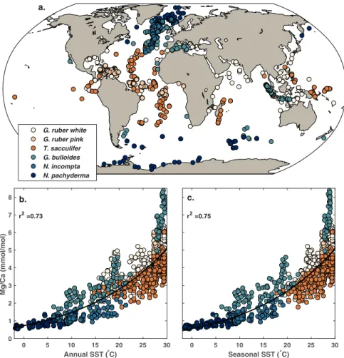
Figure 1. (a) Geographical distribution of the Mg/Ca core top data, with an “include” flag of 1 (N=1, 182), by species. (b) The relationship between Mg/Ca and mean annual SSTs. (c) The relationship between Mg/Ca and estimated seasonal SSTs. Black lines through the data in (b) and (c) represent the best fit exponential regressions, with r2_values

listed in the upper left.

excluded. We also excluded data from the eastern Mediterranean, where authigenic high-Mg coatings are commonly observed and result in anomalous Mg/Ca values (Sabbatini et al., 2011). This initial quality screen reduced our data set to 1,182 samples, with 452 core tops for G. ruber white, 74 for G. ruber pink, 292 for

T. sacculifer, 72 for N. pachyderma, 158 for N. incompta, and 134 for G. bulloides (Figure 1). G. ruber white and pink core top samples were subsequently combined and averaged and collectively treated as the G. ruber group, recognizing that these chromotypes are closely related genetically (Aurahs et al., 2011) and have sim-ilar geochemistry (Richey et al., 2012, 2019). In addition, initial exploration indicated that the G. ruber pink data set spanned a limited geographical (tropical-subtropical Atlantic) and temperature (25–28◦C) range, complicating accurate determination of regression coefficients. Likewise, N. pachyderma and N. incompta were combined and calibrated together as the N. pachyderma group. Originally considered to be morpho-types, N. pachyderma and N. incompta are now classified as genetically different species (Darling et al., 2006) and have different temperature optima (which is accounted for in our seasonal calibration). However, they have similar habitat preferences, living seasonally in the high latitudes in the mixed layer (Darling et al., 2006), and as with G. ruber pink, we found that the limited number of N. pachyderma core tops challenged calibration in isolation.

The core top data are matched to the nearest gridpoint from the World Ocean Atlas 2013 (WOA13) version 2 (Boyer et al., 2013), from which we draw mean annual and seasonal SSTs and sea-surface salinity (SSS). As with our previous calibration models for foraminiferal δ18_{O (Malevich et al., 2019), we do not}

explic-itly consider depth habitat for the different planktic groups. Although regressing against environmental parameters at 0 m water depth might not be optimal to derive the “true” sensitivities of Mg/Ca, we assume

Table 1

Sea-Surface Temperature Ranges Associated With Peak Abundances for Each Foraminiferal Species Investigated in This Study, Based on Kernel Density Estimates of Shell Fluxes From a Collection of Global Sediment Traps (from Malevich et al., 2019)

Peak abundance SST ranges (◦C)

Species Min Max Median

G. ruber 22.5 31.9 27.4 T. sacculifer 20.2 30.6 27.0 G. bulloides 3.6 29.2 18.0 N. pachyderma −0.9 15.3 5.4 N. incompta 6.7 21.1 15.3

that users want to infer past SSTs from mixed-layer species, rather than a calcification depth temperature. In addition, depth preferences tend to covary with seasonal preferences, and so accounting for both can lead to overfitting. We tested this assumption by running our Bayesian calibration models using integrated 0–50 m values; we obtained nearly identical coefficients (not shown). We note that any prescribed depth habitat in a calibration—whether it be 0 or 0–50 m—assumes that it is static in time. Circumventing this assumption requires modeling depth habitat explicitly as a function of thermal tolerance, light, and nutri-ents (e.g., Lombard et al., 2011). This adds considerable complexity, and paleoclimate applications would require biogeochemical constraints; thus, we leave this for future work.

Seasonal averages are computed using spatially varying estimates of when the peak abundance of each foraminiferal species occurs, according to their individual thermal tolerances. As described in Malevich et al. (2019), these are based on kernel density estimates (KDEs) of sediment trap data (Zari ´c et al., 2005) and the seasonal cycle in temperature at each site, as inferred from WOA13. For example, the KDE of G. ruber abundance indicates that this species prefers SSTs between 22.5 and 31.9◦C. Thus, for locations with SSTs that seasonally drop below 22.5◦C, G. ruber is assumed to not calcify during those months, and the average seasonal SST would be the mean value for all months above 22.5◦C. Effectively, this assumes that G. ruber Mg/Ca reflects mean annual SSTs at most tropical locations, but warm-season SSTs in the subtropics. We also draw seasonal optima for N. pachyderma and N. incompta separately, recognizing the distinct temper-ature preferences of these two species, even though they are ultimately calibrated together. Table 1 lists the minimum, maximum, and median SST preferences for each species according to the KDE method. For

G. ruber, T. sacculifer, and N. incompta, our inferred optimal SST ranges are very similar to those modeled by Lombard et al. (2009) from culture data (21–30◦C, 19–31◦C, and 6–20◦C, respectively). Our ranges for

G. bulloidesand N. pachyderma are slightly larger (Table 1) than the Lombard et al. (2009) estimates (10–25◦ C and 0–10◦C, respectively) because the sediment trap data indicate a wider thermal range for these species.

Core tops that fall within the same gridpoint, and contain the same species, are further averaged prior to calibration exercises to reduce the impact of spatial clustering on the regression parameters. This results in an effective core top N of 710 for our regression models, with N = 307 for G. ruber, N = 184 for T. sacculifer,

N =100for G. bulloides model, and N = 119 for N. pachyderma.

Since previous work indicates that the carbonate system influences foraminiferal Mg/Ca, we also collate surface water pH and bottom water calcite saturation state (Ω) values for each core site from the Global Ocean Data Analysis Project (GLODAP) version 2 gridded climatology (Lauvset et al., 2016). GLODAPv2 lacks coverage in the Gulf of Mexico, so for core tops in this location, we rely on bottle data collected as part of the second Gulf of Mexico and East Coast Carbon Cruise (GOMECC-2) in 2012 (data publicly available from http://www.aoml.noaa.gov/ocd/gcc/GOMECC2) and use the MATLAB implementation of CO2SYS (v1.1, Van Heuven et al., 2011) to compute pH and calcite Ω from measured values of alkalinity, dissolved inorganic carbon, salinity, temperature, pressure, silicate, and phosphate. We used the Mehrbach K1 and K2 constants, as refit by Dickson and Millero (1987).

Overall, our core top data set spans a wide range of SSTs (−1.8 to 29.6◦C; 95% CI = 3.1 to 29.4◦C) and Ω (0.7 to 5.5; 95% CI = 0.9 to 3.3). Although high and low SSS values are represented in the data set (28.4 to 38.6 psu), the distribution of the data is more restricted (95% CI = 33.3 to 37.5 psu). The range of surface water pH values sampled is limited (7.97 to 8.22; 95% CI = 8.02 to 8.17), reflecting the fact that the pH of the modern surface ocean does not have a large dynamic range.

As described below, we also use Mg/Ca data from cultured foraminifera to constrain sensitivities to envi-ronmental parameters. We use the compilation of Gray and Evans (2019), with the addition of the G. ruber pink data from Allen et al. (2016) and N. incompta data from Von Langen et al. (2005) and Davis et al. (2017). This updated culture data set includes 30 G. ruber observations, 20 T. sacculifer observations, 12 G. bulloides observations, 29 O. universa observations, and 12 N. incompta observations for a total of 103 data points.

3. Model Form and Exploration of Environmental Predictors

Temperature clearly exerts a strong, nonlinear control on core top Mg/Ca, explaining about 75% of the variance in the data (Figures 1b and 1c), in agreement with experimental evidence (e.g., Lea et al., 1999). However, laboratory studies and previous core top investigations have shown that pH, salinity, the satura-tion state (Ω) at the core site, the cleaning method, and shell size also influence Mg/Ca. Mg/Ca sensitivities to salinity and pH are also considered exponential (Evans, Wade, et al., 2016; Gray et al., 2018; Hönisch et al., 2013; Kisakürek et al., 2008; Lea et al., 1999). Culture experiments suggest a pH sensitivity of −50% to −90% per pH units for O. universa, G. bulloides, and G. ruber (white) (Evans, Brierley, et al., 2016; Gray & Evans, 2019; Lea et al., 1999; Russell et al., 2004; Kisakürek et al., 2008), and Gray et al. (2018) detected a pH sensitivity of a similar magnitude of −80 ± 70% (2𝜎) per pH units in a global compilation of G. ruber (white) sediment trap data. However, pH does not seem to impact Mg/Ca in cultures of N. pachyderma, N. incompta (Davis et al., 2017), and T. sacculifer (Allen et al., 2016). Laboratory experiments indicate a moderate sensi-tivity of planktic Mg/Ca to salinity (3–5% per psu) (Allen et al., 2016; Gray & Evans, 2019; Hönisch et al., 2013; Kisakürek et al., 2008; Lea et al., 1999). Previous core top studies suggested a much larger sensitivity (15–59%, Arbuszewski et al., 2010; Ferguson et al., 2008; Mathien-Blard & Bassinot, 2009), but reanalyses indicated that these high estimates are due either to environmental covariates (Hertzberg & Schmidt, 2013; Hönisch et al., 2013; Khider et al., 2015) or to analytical issues (Dai et al., 2019). Core top observations also reveal a systematic decline in sedimentary planktic Mg/Ca—regardless of species—under low bottom water Ω at the site of deposition (Regenberg et al., 2014). Finally, intralaboratory and interlaboratory com-parisons (Barker et al., 2003; Rosenthal et al., 2004) as well as a regression analysis of G. ruber (white) core tops (Khider et al., 2015) indicate a systematic offset in measured Mg/Ca of ∼10–15% based on whether the laboratory cleaning method includes a reductive step. Mg/Ca also varies by shell size (Elderfield et al., 2002; Friedrich et al., 2012), but researchers tend to mitigate this effect by picking foraminifera from a restricted size fraction. Preliminary investigations revealed that shell size was not a significant predictor for core top Mg/Ca, so it is not included in our models.

Since temperature, salinity, and pH sensitivities are exponential, we transform Mg/Ca to ln(Mg/Ca) for model fitting. This transformation also assumes that the errors for a Mg/Ca model follow an exponential distribution; the data in Figures 1b and 1c suggest that this is a valid assumption, as variance increases non-linearly with temperature. Following Khider et al. (2015), the cleaning parameter acts as a multiplicative term in Mg/Ca space, and thus an additive term in ln(Mg/Ca) space, with the understanding that reductive cleaning (a value of 1) results in a systematic decline in Mg/Ca. The form of the Mg/Ca dependency on Ω is less clear. Regenberg et al. (2014) and Khider et al. (2015) assume that bottom water saturation impacts Mg/Ca of tests linearly below a certain threshold, which they define based on ΔCO2−

3 instead of Ω. These

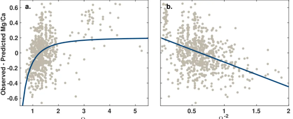
two quantities are functionally equivalent, but we prefer using Ω because it is always a positive value. How-ever, it might be expected, based on reaction kinetics, that Mg/Ca should have a nonlinear dependency on saturation state, with dissolution increasing as saturation state drops (Sjöberg, 1976). Indeed, if we remove the impact of SST on our pooled data set, we find that ln(Mg/Ca) residuals trend nonlinearly with Ω, with the slope becoming steeper as Ω becomes smaller (Figure 2). The relationship is strongest below an Ω of ∼ 1.5 (Figure 2), which is consistent with the ΔCO2−

3 threshold of ∼40 μmol/kg identified by Regenberg et al.

(2014). Ω sensitivity can be approximated by a power function, with a coefficient of −2 (Figure 2). This supports a transformation of Ω to Ω−2_{in order to linearize the sensitivity of ln(Mg/Ca) to saturation state.}

Figure 2. The relationship of core topln(Mg/Ca) residuals (observed-predicted; all species; N=710) to (a) bottom water calciteΩand (b)Ω−2_{after removing the dependence on temperature. Dots represent individual core tops; lines}

show the best fit regression.

The final form of a core top Mg/Ca forward model, based on the physical expectations outlined above, is ln(Mg/Ca) =𝛼 + T · 𝛽T+S ·𝛽S+pH ·𝛽P+ Ω−2·𝛽O+ (1 − clean ·𝛽C) +𝝐,

𝝐 ∼  (0, 𝜎2_), (1)

where𝜖 is the vector of residual errors, approximated by a normal distribution with mean zero and variance

𝜎2_.

To assess the impact of each environmental variable on model performance, we iteratively computed regres-sions using ordinary least squares, adding each predictor sequentially. We then compared the Bayesian information criterion (BIC) for each iterative model to determine whether the additional predictor resulted in improvement. The BIC is a criterion for model selection that helps guard against overfitting by penaliz-ing the addition of parameters that do not improve the model fit; lower values (regardless of sign) indicate a better fit. We also analyzed the significance of each predictor's coefficient. We do this for both the pooled data set (using annual and seasonal SST and SSS estimates) and the four species groups (using seasonal SST and SSS estimates) and discuss the results for each predictor in turn.

3.1. Temperature

For both the pooled annual and pooled seasonal data sets, we find that SST alone explains over 80% of the variance in ln(Mg/Ca) (Table 2). This is slightly greater than an exponential model for Mg/Ca (Figures 1b and 1c), reflecting some improvement in the fit associated with the assumption that variance increases expo-nentially. Temperature remains the most important parameter for the individual species models, although it explains only ca. 50% of the variance for the warm-water groups (G. ruber and T. sacculifer; Table 2). This is due to the relatively restricted temperature ranges for G. ruber and T. sacculifer (ca. 12◦C) compared to those for G. bulloides and N. pachyderma (>20◦C), which allows for more variance to be explained by the other environmental factors. The temperature sensitivity is similar across all species, between 5% and 7% (Table 2). This agrees well with recent reassessments from culture and sediment traps, both of which indi-cate a temperature sensitivity of ca. 6% (Gray et al., 2018; Gray & Evans, 2019) rather than 9%, as previously assumed (e.g., Anand et al., 2003; Dekens et al., 2002; Khider et al., 2015).

3.2. Bottom Water Calcite Saturation (𝛀)

The addition of Ω as a predictor improves almost all of the models (r2_{increases, root mean square error}

(RMSE) decreases, and BIC decreases), with the biggest impact on the warm-water species (Table 2). The large drop in BIC associated with the addition of this parameter (to the pooled models in particular, where it is about 100) supports long-standing theory and intuition that inclusion of Ω improves prediction of core top Mg/Ca (Brown & Elderfield, 1996; Dekens et al., 2002; Regenberg et al., 2014; Rosenthal et al., 2000; Rosenthal & Boyle, 1993; Russell et al., 1994). Ω sensitivity remains fairly constant across species groups, in agreement with previous work that most species of planktic foraminifera are sensitive to saturation state at the site of deposition (Regenberg et al., 2014). The possible exception is the N. pachyderma group, for

Table 2

Regression Model Metrics and Coefficients

SST +Ω−2 _{+ clean + SSS −SSS +pH} Pooled annual, n=710 r2 _{0.83 0.86 0.87 0.87 0.87} RMSE 0.24 0.22 0.21 0.21 0.21 BIC 2 −135 −198 −210 −193 Coefficient 0.063 −0.35 0.16 0.029 0.30 Pooled seasonal, n=710 r2 _{0.85 0.87 0.89 0.89 0.89} RMSE 0.22 0.21 0.19 0.19 0.19 BIC −114 −210 −293 −288 −289 Coefficient 0.064 −0.27 0.17 -0.004 0.36 G. ruber, n=307 r2 _{0.55 0.66 0.71 0.71 0.71} RMSE 0.15 0.13 0.12 0.12 0.12 BIC −284 −363 −407 −403 −404 Coefficient 0.068 −0.24 0.11 0.002 0.28 T. sacculifer, n=184 r2 0.51 0.68 0.73 0.73 0.77 RMSE 0.13 0.11 0.10 0.10 0.09 BIC −214 −287 −318 −314 −339 Coefficient 0.055 −0.27 0.12 0.006 1.4 G. bulloides, n=100 r2 0.86 0.88 0.88 0.89 0.89 RMSE 0.19 0.17 0.17 0.17 0.17 BIC −44 −60 −57 −54 −55 Coefficient 0.068 −0.29 0.12 −0.024 −1.0 N. pachyderma, n=119 r2 _{0.78 0.79 0.80 0.80 0.80} RMSE 0.15 0.15 0.15 0.15 0.15 BIC −109 −107 −108 −106 −106 Coefficient 0.052 -0.06 0.088 0.047 0.57 Note.Each column notes the addition (or subtraction) of a predictor relative to the column to the left. Group-specific models were calculated with seasonal tem-perature and salinity estimates. Lower values indicate improved performance. ndenotes the number of core tops (after gridding, see section 2). Coefficients correspond to that of the added predictor. Coefficients in italics are not signif-icantly different than zero (at p=0.05). BIC = Bayesian information criterion; RMSE = root mean square error (inln(Mg/Ca) units).

which Ω is not a significant predictor (Table 2). Ω ranges between 0.75 and 2.8 within this group; hence, the lack of sensitivity does not reflect a limitation of the data. It may be that N. pachyderma and N. incompta, which have a thicker outer calcite crust than the other species considered here, are indeed less sensitive to dissolution, in agreement with buoy exposure experiments (Berger, 1970), although the error on the Ω coefficient is large (±0.1, 2𝜎).

3.3. Cleaning

The addition of the cleaning parameter (0 for samples without the reductive step, 1 for samples with the reductive step) improves the statistics for the pooled models and the warm-water groups, with drops in BIC on the order of 10–50 (Table 2) but has little impact on G. bulloides and N. pachyderma. In the case of G. bulloides, this reflects a limitation of the data subset: All but two of the core tops were cleaned with the oxidative protocol, so it is not possible to reliably detect the influence of reductive cleaning. For

N. pachyderma, the influence of cleaning on model skill is small, but the derived coefficient (9%) is close to the other species (11–12%) and is in agreement with previous estimates (Barker et al., 2003; Khider et al., 2015; Rosenthal et al., 2004). Overall, the change in BIC suggests that inclusion of laboratory cleaning does notably improve prediction of core top Mg/Ca and, the limitation of the G. bulloides data subset aside, the sensitivity should be relatively consistent across species, as expected from laboratory investigations (Barker et al., 2003).

3.4. Salinity

The addition of salinity to the model does not significantly improve the statistics for the species group regressions, nor for the pooled seasonal model (BIC is mostly unchanged; Table 2). The inferred sensitiv-ity to salinsensitiv-ity is low or statistically insignificant in all of these cases. There is moderate improvement in the pooled annual model (BIC drops by 12), and the inferred sensitivity is higher (2.9% per psu), consis-tent with the best estimate from culture studies (3.6 ± 1.2%, 2𝜎; Gray & Evans, 2019). Overall, these results suggest that the addition of salinity neither improves nor degrades core top Mg/Ca prediction, and further-more that the derived salinity sensitivity from the core top data set is essentially negligible. This result is not due to our choice to calibrate to surface salinity; derived sensitivities from 0 to 50 m average values yield equally low values (not shown). Rather, the accuracy of the derived salinity sensitivities is restricted by both the limited range of values in our core top data set (95% CI = 33.3 to 37.5 psu) and the strong covariation between temperature and salinity that is typical of global ocean. Since the high latitudes are fresh and cold, and the subtropics warm and salty, below SSTs of 21◦C, SST and SSS are positively correlated in our data set (𝜌 = 0.87, p < 0.0001). Since the tropics are warm and fresh, above 21◦C SST and SSS are negatively correlated (𝜌 = −0.73, p < 0.0001). Even though the direction of the correlation flips, this high degree of relation creates a condition of collinearity, especially for the group data subsets as they fall on one side of the relationship or the other. This means that the OLS-derived coefficients for SSS are not reliable.

3.5. pH

The addition of pH degrades model performance and/or yields insignificant or unrealistic coefficients (Table 2). The expected sensitivity from laboratory experiments is −70 ± 14% per pH unit; in comparison, our coefficients are generally of the incorrect sign (Table 2). This is unsurprising given the restricted range of values (8.02–8.17, 95% CI) in our data set and, more broadly, in the modern ocean. In addition, pH is collinear with temperature (r = −0.70, p < 0.0001), because cold locations have a higher pH. It is also pos-sible that the water column pH observations derived from the GLODAPv2 product are inaccurate. Point GLODAP measurements from the upper water column may not fully sample seasonal and year-to-year vari-ability and include the impact of anthropogenic CO₂, which, in most locations, would not be represented in core top Mg/Ca values. Overall, our regression analysis demonstrates that Mg/Ca sensitivity to pH cannot be reliably recovered from core top data.

3.6. Summary of Environmental Sensitivities

Our iterative regression analysis identifies temperature, Ω, and the laboratory cleaning method as significant predictors of core top Mg/Ca. Salinity and pH sensitivities cannot be accurately determined from the core top data set due to collinearity, a limited range of values, and possible inaccuracies in observations. From an empirical point of view, these findings support the omission of salinity and pH from the Mg/Ca model. However, it is well known from culture studies that salinity and pH are important influences on Mg/Ca and can bias estimates of past temperatures (Gray & Evans, 2019; Khider et al., 2015). We therefore retain these predictors, but in order to provide better constraints on their coefficients, we develop Bayesian hierarchical models in which both the culture and core top data are used to constrain parameters. This model struc-ture leverages the information in both the experimental (laboratory) data and the empirical (core top) data, ultimately allowing for more accurate prediction of Mg/Ca.

4. BAYMAG: Bayesian Calibration Models for Mg/Ca

4.1. Model Design

Following our previous work with𝛿18_{O of foraminifera (Malevich et al., 2019), we developed two styles}

of forward models to represent core top Mg/Ca: one that pools all species together (mainly for deep-time applications with extinct species) and another that treats each species group separately, with information

shared through parameters and hyperparameters. The pooled model design is ln(Mg/Cac) =

{

𝛼i+Tc·𝛽Tc+Sc·𝛽S+𝜖c if incompta, sacculi𝑓er 𝛼i+Tc·𝛽Tc+Sc·𝛽S+pHc·𝛽P+𝜖c if ruber, bulloides, universa 𝜖c∼ (0, 𝜎2

ci),

(2)

ln(Mg/Ca) =𝛼 + T · 𝛽T+S ·𝛽S+pH ·𝛽P+ Ω−2_{·𝛽O+ (1 − clean ·𝛽C) +𝜖,}

𝜖 ∼  (0, 𝜎2₎ (3)

with different values of𝛼 and 𝜎 for each i cultured species. Hyperparameters on the culture temperature coefficient are

𝛽Tc∼ (𝜇𝛽T, 𝜎

2

𝛽T), (4)

and the culture temperature coefficient acts as a prior on the core top temperature coefficient:

𝛽T∼ (𝛽Tc, 𝜎_𝛽T2 ). (5)

The top of the model hierarchy (equation (2)) describes Mg/Ca in the culture data set (see section 2 for a description of the data compilation) and accounts for the fact that Mg/Ca in cultures of N. incompta and

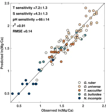
T. sacculiferis not sensitive to pH (Allen et al., 2016; Davis et al., 2017). Otherwise, the temperature, salinity, and pH sensitivities are assumed to be similar across cultured species, while the intercept and error terms are allow to vary between each species i to account for offsets in the mean and variance of ln(Mg/Ca). As a reality check, we run this top part of the model independently to assess how well it predicts culture Mg/Ca data alone. We find that this top hierarchy yields excellent prediction and the posterior coefficients for tem-perature, salinity, and pH are similar to previous assessments done with an ordinary least squares approach (Gray & Evans, 2019) (Figure 3), validating our model design.

The lower part of the hierarchy (equation (3)) contains the model for the core top data. Since the core tops are pooled together across all species, it assumes a generic pH sensitivity. The pH and salinity sensitivities (𝛽Pand𝛽S) are constrained by the culture data in the top part of the hierarchy and then allowed to influence the core top data. Conversely, the sensitivities to Ω and the cleaning method (𝛽Oand𝛽C) are only constrained by the core top data. The temperature sensitivities𝛽T_cand𝛽Tare constrained by both the culture and core top data, with the former acting as the prior mean for the latter.

The group-specific core top model takes the slightly modified form, ln(Mg/Ca_c) =

{

𝛼i+T_c·𝛽Tc+S_c·𝛽S+𝜖c if incompta, sacculi𝑓er 𝛼i+Tc·𝛽Tc+Sc·𝛽S+pHc·𝛽P+𝜖c if ruber, bulloides, universa 𝜖c∼ (0, 𝜎2_ci),

(6)

ln(Mg/Ca) =

{

𝛼𝑗+T ·𝛽T+S ·𝛽S+ Ω−2·𝛽O+ (1 − clean ·𝛽C) +𝜖 if pach𝑦, sacculi𝑓er 𝛼𝑗+T ·𝛽T+S ·𝛽S+pH ·𝛽P+ Ω−2·𝛽O+ (1 − clean ·𝛽C) +𝜖 if ruber, bulloides 𝜖 ∼  (0, 𝜎2

i)

(7) with hyperparameters and priors on the temperature coefficients as above (equations (4) and (5)). The top part of the hierarchy (equation (6)), describing the culture data, is identical to the pooled model (equation (2)). The lower part of the hierarchy (equation (7)) describes the core top data and, since species are treated independently, accounts for the fact that the T. sacculifer and N. pachyderma core tops should not be sensitive to pH. As with the culture data, the intercept and error terms (𝛼jand𝜎j) are allowed to vary for each j foraminiferal species. The temperature, salinity, Ω, and cleaning sensitivities are computed across all of the data and are not allowed to vary by species. This choice was made because our regression experiments indicated that, with few exceptions, these sensitivities are similar across species (Table 2). Although we did observe a lower Ω sensitivity for the N. pachyderma group (see section 3.2), computation of a hierarchical model with group-specific Ω coefficients yielded no improvement in model skill. Likewise, computation of

Figure 3. Bayesian hierarchical model results for planktic Mg/Ca culture

data, including median and 2𝜎ranges for the posterior temperature, salinity, and pH sensitivities.

group-specific temperature coefficients did not improve skill, supporting our assumption (and inferences from the culture data) that temperature sensitivity should be similar across species.

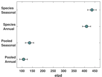
For all models, we estimate parameters using Bayesian inference and Markov chain Monte Carlo sampling (Gelman et al., 2003) with Stan soft-ware, version 2.19.1 (Carpenter et al., 2017). Prior distributions for the parameters and hyperparameters, as well as prior versus posterior plots, are given in Appendix A. To assess the impact of using annual versus seasonal SST and SSS, we computed the pooled and group-specific mod-els with both sets of values, although we recommend use of either the pooled annual or group-specific seasonal models for practical applica-tions. We perform Pareto-smoothed importance sampling leave-one-out cross-validation to compare predictive accuracy between models (Vehtari et al., 2017). These values are reported as expected log pointwise predic-tive density (elpd); larger values indicate a better fit to the data.

4.2. Model Results

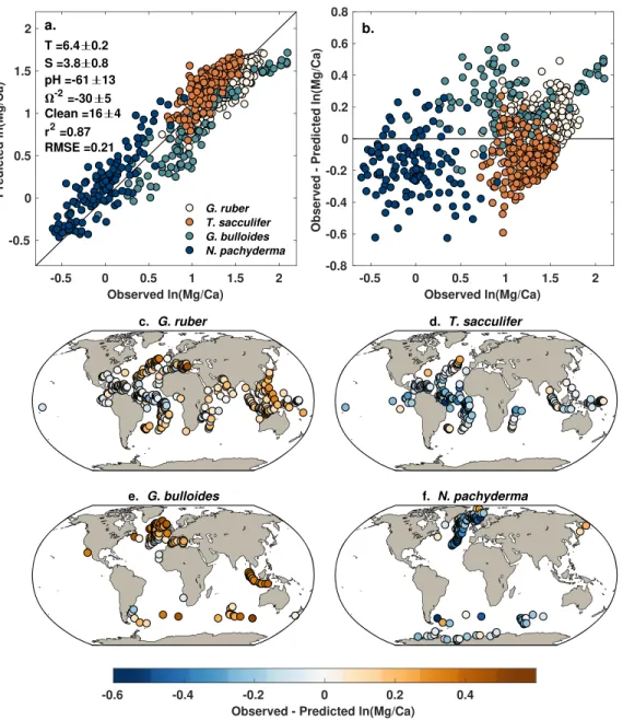
The pooled annual model explains 87% of the variance in the core top Mg/Ca data and has a median RMSE of 0.21 ln(Mg/Ca) units (Figure 4a). Analysis of the Mg/Ca residuals yields no significant trends with the SST, SSS, Ω, and cleaning predictors. There is a weak correlation between the residuals and core top pH (Spearman's𝜌 = 0.15, p < 0.0001), but as discussed above, we are unsure whether the core top pH observations are accurate. Likewise, the posterior coefficients for the pH predictor are very similar to the those derived from the culture data alone (Figure 3) reflecting limited influence from the core top data. The derived salinity sensitivity is also close to cul-ture expectations at 3.8%. The median temperacul-ture coefficient is lower than the culcul-ture value (6.4 vs. 7.2) although by design, is still the same within uncertainty. This shift reflects the influence of the core top data, which act to narrow the temperature sensitivity down to a precise estimate of 6.4 ± 0.2 (2𝜎).

While as a whole the residuals are well distributed across the zero line, there are systematic offsets accord-ing to species (Figure 4b). This is expected, as neither seasonality nor species differences are accounted for in the pooled model. Generally speaking, the model overpredicts Mg/Ca for N. pachyderma and T. sacculifer (Figures 4d and 4f) and underpredicts Mg/Ca for G. ruber and G. bulloides (Figures 4c and 4e). These species-level offsets likely reflect differences in depth habitat. N. pachyderma is typically interpreted to inhabit the upper 100 m of the water column (Elderfield & Ganssen, 2000; Mortyn & Charles, 2003; Reynolds & Thunell, 1986; Taylor et al., 2018), which would integrate cooler temperatures than SST and lead to lower observed ln(Mg/Ca). This may explain model overestimation in the high latitudes (Figure 4f). Likewise, in the tropics T. sacculifer is often found in a slightly deeper habitat than G. ruber (Erez & Honjo, 1981; Fairbanks et al., 1980; Ravelo & Fairbanks, 1992), leading to lower Mg/Ca than predicted from surface tem-peratures. This expected offset between G. ruber and T. sacculifer can be seen visually in Figure 4a; at higher values of ln(Mg/Ca), T. sacculifer plots to the left of G. ruber. This explains model overestimation in the tropics (Figure 4d). The pooled model underestimates G. bulloides Mg/Ca nearly everywhere, because this species tends to have higher average Mg/Ca values than N. pachyderma, G. ruber, and T. sacculifer (Cléroux et al., 2008; Elderfield & Ganssen, 2000) (Figure 4e).

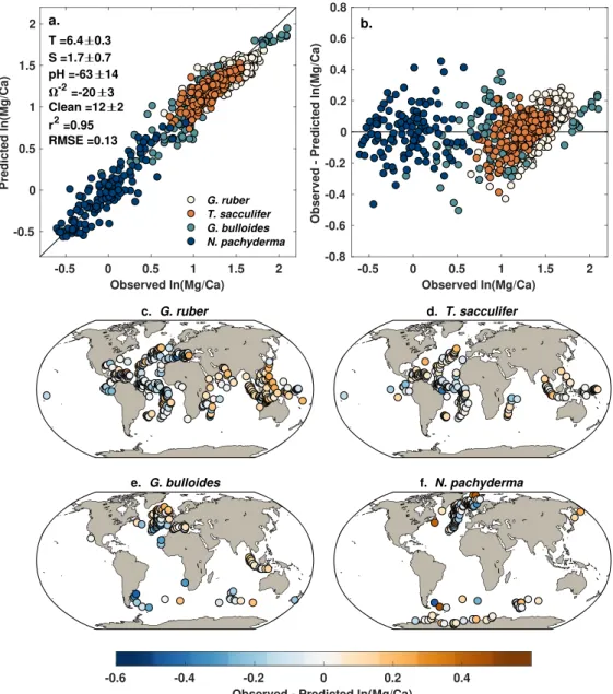
It is not surprising then that model performance improves markedly with the use of seasonal SST and SSS and group-specific parameters. The most significant improvement comes from accounting for differences between foraminiferal groups (equation (7)), which cause elpd, a measure of predictive accuracy, to rise from 100–150 to 400–450, indicating a much improved fit (Figure 5). The seasonal, group-specific model can account for 95% of the variance in the core top data (Figure 6) with an RMSE comparable to that of the culture regression (Figure 3). As with the pooled model, there is no significant correlation between the cleaning and Ωpredictors and the residuals and a weak positive correlation with the pH predictor (𝜌 = 0.11, p = 0.003). There are however weak correlations between the residuals and both temperature and salinity (𝜌 = 0.13,

p = 0.0008; 𝜌 = −0.21, p < 0.0001). The negative correlation with salinity is seen in all species groups except T. sacculifer and represents the model balance between the strong salinity sensitivity inferred from the

Figure 4. Pooled annual model results. (a) Observed versus predicted ln(Mg/Ca), including posterior coefficients for

each environmental predictor, colored by species group. (b) Model residuals, colored by species group. (c–f) Maps of model residuals for each species group.

culture data (4.3%, Figure 3) and the weak salinity sensitivity that is recovered from the core top data when seasonal SSTs are used (Table 2). As discussed in section 3.4, the core top-derived salinity sensitivities are affected by collinearity between SST and SSS and therefore may not be accurate. To enforce a sensitivity that is consistent with the culture data, we applied an informative prior to the salinity parameter (see Appendix A). The posterior salinity coefficient is still significantly smaller than that of the pooled model (1.7 ± 0.7 vs. 3.8 ± 0.8) due to core top influence but is higher than it otherwise would be without this constraint. The correlation between residuals and temperature seems to be mostly driven by G. ruber residuals, which also show a strong trend with observed ln(Mg/Ca) (r = 0.70, p < 0.0001). This could indicate that temperature sensitivity for G. ruber is systematically underestimated; however, the trend is only slightly ame-liorated after running a version of the group-specific model with variable SST coefficients for each species (r = 0.61, p < 0.0001), and the derived ca. 6% sensitivity of the seasonal group-specific model is very sim-ilar to values calculated from G. ruber culture and sediment trap data (Gray & Evans, 2019; Gray et al., 2018). Alternatively, this residual trend could suggest that our relatively simple inference of seasonal SST

Figure 5. Expected log pointwise predictive density (elpd), based on

Pareto-smoothed importance sampling leave-one-out cross-validation, for each Bayesian model. Higher values indicate better fit.

(based on sediment trap abundances) does not apply well to G. ruber. However, we did not see this residual trend in our model for𝛿18_{O of}

G. ruber, which uses the same seasonal estimation method (Malevich et al., 2019). Accounting for subtle differences in depth habitat would make the trend worse, as studies suggest that G. ruber should have a deeper habitat in the tropics (and therefore lower Mg/Ca) and shal-lower one in the subtropics (and therefore higher Mg/Ca) (Hertzberg & Schmidt, 2013; Hönisch et al., 2013). Similar to G. ruber, a group of

G. bulloides data with very high Mg/Ca also falls to the right of the one-to-one line (Figure 6). These data are from the Sumatran margin, where G. bulloides calcifies primarily during the cooler upwelling season, at a depth of ca. 50 m (Mohtadi et al., 2009). This preference should cause negative, rather than the observed positive, residuals. Taken together, the G. bulloides and G. ruber residuals suggest that Mg/Ca sensitivity to temperature may, in fact, be more nonlinear than our model (and all previous exponential models) have assumed or alternatively that there is a latent environmental variable or vital effect that scales nonlinearly with temperature. This latent effect is most prominent in G. ruber and accounts for the fact that our model can only explain 67% of the variance in G. ruber Mg/Ca. In contrast, our model can explain 73%, 88%, and 77% of the variance in Mg/Ca for T. sacculifer, G. bulloides, and N. pachyderma, respectively.

Further investigation is needed to properly diagnose what this latent variable might be, but the fact that impacts G. ruber and G. bulloides preferentially suggests that it could be pH. pH scales inversely with tem-perature; warm locations have lower pH and would be associated with higher Mg/Ca than expected from temperature alone. Although pH is included in our model, if the GLODAP measurements are inaccurate, then this effect would not be fully accounted for in our Mg/Ca predictions and produce the kind of residual trends we observe. Indeed, tropical regions, such as the eastern equatorial Pacific and Indo-Pacific warm pool, are poorly observed in the GLODAP data set, and these are also locations where the residual error is notably low and high, respectively, for G. ruber (Figure 6c).

In spite of the residual trends, the magnitude of the residual bias is still very small (0.13 ln(Mg/Ca) units, 1𝜎), and out-of-sample applications of BAYMAG in section 5 suggest that our model yields good prediction of G. ruber Mg/Ca.

The seasonal group-specific model eliminates the species-level offsets seen in the pooled annual model by allowing the intercept terms to vary for each foraminiferal group (Figure 6b). These intercept terms effectively compensate for depth habitat preference as well as any offsets in average Mg/Ca incorpora-tion. Many of the strong spatial trends in residuals are also minimized (Figures 6c–6f) when compared to the pooled model (Figures 4c–4f), although some patterns remain. In addition to patterns that may reflect the impact of the latent variable discussed above, there are negative residuals for G. bulloides in the west African and Benguela upwelling zones; along frontal regions in the Southern Ocean; and near the con-fluence of the Brazil and Malvinas currents (Figure 6e) indicating that Mg/Ca values are lower than the model predicts. Similar patterns were observed in the residuals of our Bayesian δ18_{O models (Malevich et al.,}

2019) and might suggest that G. bulloides is calcifying during either a cooler season than our seasonal SST inferences predict or in a deeper habitat. These patterns could also conceivably reflect geochemical differ-ences between G. bulloides genotypes (Sadekov et al., 2016) or high productivity driving locally enhanced dissolution (Hertzberg & Schmidt, 2013).

5. Application of the BAYMAG Forward Model

Forward modeling of Mg/Ca is useful for model-data comparison and data assimilation techniques that rely on forward models to translate model output into proxy units (Hakim et al., 2016). BAYMAG can be used to model new values of Mg/Ca (̃𝑦) from observed or simulated SST, SSS, pH, Ω, and cleaning protocol by simply drawing from the posterior predictive distribution,̃𝑦 ∼  (𝜇, 𝜎2_{), where𝜇 and 𝜎 are the core top component}

Figure 6. Seasonal, group-specific model results. (a) Observed versus predicted ln(Mg/Ca), including posterior

coefficients for each environmental predictor, colored by species group. (b) Model residuals, colored by species group. (c–f) Maps of model residuals for each species group.

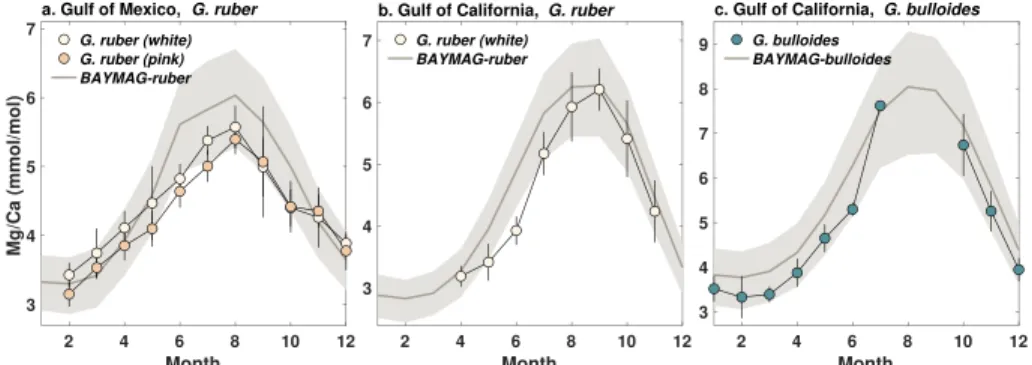
of either the pooled annual or group-specific seasonal model (equations (3) and (7)). If the user desires, a prior can be used to restrict values to reasonable outcomes; for example, for G. ruber, Mg/Ca values over 6.5 are rarely observed in the modern ocean (0% of core tops and 1% of sediment traps). To provide an example, as well as to test our model on out-of-sample data, we apply BAYMAG to monthly average observations of SST, SSS, and pH at two locations that have multi-year foraminiferal Mg/Ca sediment trap data (Figure 7). For the Gulf of Mexico site, we used the SST, SSS, and pH climatologies (adjusted values) provided in the source publication (Richey et al., 2019). For the Gulf of California site, we used average monthly SSTs reported in the source publication (McConnell & Thunell, 2005), WOA13 climatology for SSS, and pH climatology as estimated by Gray et al. (2018). Ω is set to 5.7 for the Gulf of Mexico and 3.4 for the Gulf of California; since these values are high, they have minimal impact on predicted Mg/Ca. Both studies used a nonreductive cleaning protocol, so the cleaning value is set to 0. In all cases we use the group-specific, seasonal model; although temperatures and salinity vary month by month in this case, we assume that the seasonal model most accurately captures the “true” environmental sensitivities. Weak priors on Mg/Ca were used to assign a low probability (< 5%) to Mg/Ca values above 7 and 9 for G. ruber and G. bulloides, respectively (Figure 7).

Figure 7. Forward-modeled Mg/Ca from BAYMAG, compared to sediment trap observations from the Gulf of Mexico

(Richey et al., 2019) and Gulf of California (McConnell & Thunell, 2005). Normal priors of ∼ (4, 1.5)and ∼ (5, 2) were used for G. ruber and G. bulloides, respectively. The Gulf of Mexico data were shifted backwards by 1 month to account for sinking and integration time. No adjustments to the Gulf of California data were made; this is a shallower trap (485 vs. 1,150 m), and the data indicate minimal lag. Shading and error bars represent1𝜎uncertainties.

Overall, the BAYMAG predictions match observed Mg/Ca values well, almost always overlapping within the 1𝜎 range (Figure 7). This is an encouraging result, because our model is calibrated on core top foraminifera that have been affected by dissolution and sedimentary processes, while the sediment trap data consist of more pristine specimens. BAYMAG slightly overestimates G. ruber Mg/Ca in the Gulf of Mexico (Figure 7a), even though our model residuals suggest that it should underpredict high values (Figure 6b), suggesting that the residual trends have a minimal impact on prediction.

6. Inversion of BAYMAG to Predict Past SST

Since BAYMAG is a multivariate model, inversion to predict past SSTs requires constraints on salinity, pH, and Ω. In the simplest case, these can be held constant at modern values, but this assumes that only temper-ature caused observed variation in Mg/Ca. More realistic inference can be derived from making informed assumptions about past changes. For example, over the Quaternary glacial cycles, it is reasonable to assume that surface water pH and salinity both increased during glacial periods due to lower atmospheric CO2and

lower sea level. It is also possible to leverage information from independent proxies sensitive to changes in the oceanic carbonate system, such as𝛿11_{B (for surface pH) or benthic B/Ca (for Ω). Alternatively, output}

from a climate or biogeochemical model could be used to provide constraints.

To facilitate SST prediction for diverse applications, we provide two versions of the Bayesian inverse model for Mg/Ca. One assumes that salinity, pH, and Ω are known, allowing for quick computation of posterior SST. The other treats all of the environmental predictors as unknowns and allows the user to place prior dis-tributions on them. This latter model involves joint computation of posterior temperature, salinity, pH, and Ωand is therefore slower to converge but has the advantage of propagating uncertainty in these covariates into the estimation of SST.

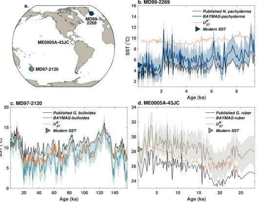
To demonstrate use of the inverse models, we apply BAYMAG to three sites that have Late Quaternary Mg/Ca data as well as independent estimates of SST from alkenone UK′

37 (Figure 8a). In each case, we use

the appropriate seasonal, group-specific model; however, our KDE method for inferring seasonality predicts that foraminifera at all three of these locations should reflect mean annual temperature. We draw modern Ω and surface pH value for each site from GLODAPv2 (Lauvset et al., 2016) and modern salinity from WOA13 (Boyer et al., 2013). In all cases, we use a prior standard deviation of 6◦C and assume that pH, salinity, and Ω are error free; we found that including errors on these factors only slightly increases error bars (not shown). For the Holocene data at site MD99-2269 in the North Atlantic, we assume that salinity, and Ω are constant through time (N. pachyderma is not sensitive to pH). We find that BAYMAG predicts latest Holocene SST values that are in good agreement with modern observed annual SST, whereas the calibration (Elderfield & Ganssen, 2000) used in the original publication (Kristjánsdóttir et al., 2017) slightly underestimates SSTs (Figure 8b). The BAYMAG predictions suggest that annual SSTs have declined through the Holocene by about 3◦C. In contrast, the UK′

Figure 8. Example applications of BAYMAG to predict past SSTs. (a) Locations of targeted Late Quaternary sites.

(b) N. pachyderma data from MD99-2269 (66.6◦N, 20.9◦W, 365 m, Kristjánsdóttir et al., 2017). (c) G. bulloides data from MD97-2120 (45.5◦S, 174.9◦E, 1210 m, Pahnke et al., 2003). (d) G. ruber data from ME0005A-43JC (7.9◦N, 83.6◦W, 1368 m, Benway et al., 2006). At each location, data are compared to UK′

37SST estimates (median values, calibrated with

BAYSPLINE, Tierney & Tingley, 2018). Triangles show modern mean annual SSTs at each site. Shading indicates1_𝜎

uncertainties.

than the N. pachyderma predictions (Figure 8b). UK′

37at this latitude (66◦N) is assumed to reflect late summer

temperatures (August–October) (Tierney & Tingley, 2018); however, modern August–October SSTs at this site (6.4◦C) are still much cooler than the latest Holocene UK′

37 values (ca. 9.5◦C, Figure 8b). This might

indicate that UK′

37 production is restricted to only the warmest of summer months; alternatively, the warm

bias could reflect the influence of sea ice. This site sits close to the boundary where substantial seasonal sea ice is present in the modern day, and anomalously high UK′

37values occur in areas of extensive sea ice cover

(Filippova et al., 2016; Tierney & Tingley, 2018).

For site MD97-2120 in the South Pacific, we make some rudimentary assumptions of how pH and salinity may have varied over glacial-interglacial cycles. Following Gray et al. (2018) and Gray and Evans (2019), we assume that global pH increased by 0.13 units during the Last Glacial Maximum (LGM) due to lowered CO2. We then scaled the normalized ice core CO2curve (Bereiter et al., 2015) to this value and added it to

the modern site estimate of pH to simulate past changes. For this site, this results in a range of pH values between 8.12 (modern value) and 8.25 (maximum glacial value). For salinity, we scaled the normalized sea level curve to an inferred LGM change of 1.1 psu and added this to the site estimate, for a range between 34.4 (modern values) and 35.5 (maximum glacial value). We then interpolate these scaled curves to the ages at which there are Mg/Ca observations and input them into BAYMAG. We do not explicitly account for the temperature effect on pH (e.g., Gray & Evans, 2019) because while it scales with the magnitude of local cooling, it is a small source of error for the LGM (0.65◦C, Gray & Evans, 2019). Since the salinity and pH sensitivities are of opposite sign, the glacial-interglacial changes partly cancel each other out; however, LGM cooling is still 0.8◦C warmer than estimates made with constant salinity and pH (not shown) due to the pH effect.

The BAYMAG predictions from G. bulloides Mg/Ca at MD97-2120 produce latest Holocene SSTs in good agreement with modern mean annual values and yield cooler median values and a larger glacial-interglacial

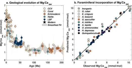
Figure 9. (a) Evolution of Mg/Caswover the past 200 Ma, according to Mg/Ca measured in calcium carbonate veins

(CCV, Coggon et al., 2010), fossil corals (Gothmann et al., 2015), echinoderm ossicles (Dickson, 2002; Dickson, 2004), halite fluid inclusions (Brennan et al., 2013; Horita et al., 2002; Lowenstein et al., 2001), and large benthic foraminifera (LBF, Evans et al., 2018). Star denotes the modern value of 5.2 mmol/mol (Horita et al., 2002). Shading encloses the 95% CI of an ensemble of Gaussian smoothed fits to the data, used in the seawater-enabled BAYMAG models. (b) Relationship between observed Mg/Ca_swand linear predictions of Mg/Ca_swfrom Mg/Ca of calcite in laboratory inorganic precipitation (Mucci & Morse, 1983) and foraminiferal culture studies (De Nooijer et al., 2017; Delaney et al., 1985; Evans et al., 2015; Evans, Brierley, et al., 2016; Hauzer et al., 2018; Mewes et al., 2014; Raitzsch et al., 2010; Segev & Erez, 2006).

range than the calibration (Mashiotta et al., 1999) used in the original publication (Pahnke et al., 2003) (Figure 8c). There is generally a good match with alkenone UK′

37, except during the coldest times of the glacial

periods (Figure 8c). The cold predictions in part reflect the fact that the glacial G. bulloides Mg/Ca values at this site are at the limit of the modern calibration data set, and the group-specific model has a tendency to overpredict Mg/Ca (and thus underpredict SSTs) at southern latitudes (Figure 6e). A tighter prior could mitigate this effect; however, this example illustrates that caution should be exercised when extrapolating BAYMAG to values of Mg/Ca that are near the edge or outside of the calibration range.

Finally, we tested BAYMAG on G. ruber data from site ME0005A-43JC, in the eastern Pacific warm pool. We scale salinity and pH estimates in the same manner as at site MD97-2120. Varying salinity and pH results in glacial estimates that are ca. 0.9◦C warmer than a constant assumption (not shown). Latest Holocene BAYMAG predictions once again align well with modern SSTs and are overall warmer than the published estimates (Benway et al., 2006), which used the Anand et al. (2003) calibration without a correc-tion for dissolucorrec-tion (Figure 8d). Although this site is not particularly deep, it sits in a relatively corrosive location—modern Ω is 0.95—thus, BAYMAG assumes some Mg/Ca loss from dissolution. The magnitude of glacial cooling agrees well with the UK′

37 estimates, although the two proxies have different trajectories

through the deglaciation and the Holocene (Figure 8d). The different trajectories could reflect differences in the seasonal production of alkenones and G. ruber (Timmermann et al., 2014); however, core top studies in the eastern equatorial Pacific do not find any evidence for a seasonal bias in alkenone signatures (Kienast et al., 2012; Tierney & Tingley, 2018).

7. Use of BAYMAG on Longer Geological Timescales

7.1. Incorporating Changes in Mg/Ca of Seawater

When Mg/Ca is used to infer SSTs on million-year timescales, data must be corrected for secular changes in the Mg/Ca ratio of seawater (Mg/Casw). Ancient Mg/Caswvalues can be independently estimated from fossil

corals (Gothmann et al., 2015), halite fluid inclusions (Brennan et al., 2013; Horita et al., 2002; Lowenstein et al., 2001), calcium carbonate veins (Coggon et al., 2010), echinoderm ossicles (Dickson, 2002; Dickson, 2004), and paired Mg/Ca-clumped isotope measurements of benthic foraminifera (Evans et al., 2018). Although some of these Mg/Caswestimates have large uncertainties and are also sometimes poorly dated,

they clearly indicate a nonlinear increase in Mg/Casw over the past 200 Ma, with the most rapid change

occurring in the last 30 Ma (Figure 9a). The reason for the increase is still not certain; magnesium isotope evidence and geochemical modeling suggest that it could reflect a decrease in Mg incorporation into marine clays (Dunlea et al., 2017; Higgins & Schrag, 2015).

To develop a version of BAYMAG that accounts for changing Mg/Ca_sw, we created a 1,000-member ensem-ble of possiensem-ble Mg/Ca_swtrajectories by Monte Carlo sampling the uncertainties in both age assignment and Mg/Ca_swof each estimate in Figure 9a, interpolating to a 0.5 Ma time step, and applying a 13 Ma (the resi-dence time of Mg) Gaussian smooth (Figure 9a). The resulting collection of curves is then used to calculate Mg/Caswfor each time t for a given Mg/Ca data series and then used in the prediction model, that is:

ln(Mg/Ca) =𝛼_𝑗+T ·𝛽T+S ·𝛽S+pH ·𝛽P+ Ω−2·𝛽O+ (1 − clean ·𝛽C) + Mg/Caswt Mg/Ca_sw0 +𝜖,

𝜖 ∼  (0, 𝜎2

i).

(8)

Previous work has suggested that the incorporation of Mg into calcite varies nonlinearly with Mg/Casw,

necessitating a power function correction (Evans & Müller, 2012), rather than a simple ratio between the past value and the modern value as we suggest above. To re-examine whether such an adjustment is neces-sary, we compiled experimental data in which planktic and benthic foraminifera were cultured at varying Mg/Caswconcentrations (De Nooijer et al., 2017; Delaney et al., 1985; Evans et al., 2015; Evans, Brierley, et al.,

2016; Hauzer et al., 2018; Mewes et al., 2014; Raitzsch et al., 2010; Segev & Erez, 2006), along with an inor-ganic precipitation experiment (Mucci & Morse, 1983) (Figure 9b). These data span values of Mg/Ca_swfrom 0.5 to 10 mmol/mol (Figure 9b), which encompasses the range found throughout the Phanerozoic (0.5–6 mmol/mol, Dickson, 2002; Dickson, 2004). For each species (and the inorganic experiment), we computed an ordinary least squares regression between Mg/Caswand Mg/Cacand used the resulting coefficients to

predict Mg/Caswfrom Mg/Cac. If there were a nonlinear relationship between Mg/Caswand Mg/Cac, then

the predictions should show curvature away from the the 1:1 line. We find that when all the experiments are considered together, this is not the case—a power function fit to the predictions, of the form y = a × xb_,

yields a value of b close to 1 (0.97 ± 0.07, 2𝜎) suggesting no significant curvilinear behavior. Power fits to predictions from individual species (and the inorganic experiment) also yield values of b insignificantly dif-ferent from 1, confirming that the relationship between Mg/Caswand Mg/Cacis adequately described by a

linear function. The slope of this relationship varies substantially between species; however, since Mg/Casw

is ratioed to the modern value (equation (8)), this term cancels out. This analysis does not preclude nonlin-ear incorporation of Mg into calcite at very low Mg/Ca_swconcentrations (<0.5 mmol/mol); however, such concentrations are not observed in the Phanerozoic. Thus, we conclude that a power function adjustment is not necessary for paleoclimate applications.

More recently, it has been proposed that the temperature sensitivity of Mg/Ca in foraminifera changes with Mg/Ca_sw(Evans, Brierley, et al., 2016). However, thus far this has only been detected in a culture experi-ment of G. ruber; a study of benthic foraminiferal species did not detect a change in temperature sensitivity with Mg/Casw(De Nooijer et al., 2017). We therefore do not incorporate this aspect into our model; further

experimental evidence supporting this effect is needed.

7.2. Applications

To test our Mg/Ca_sw-enabled models, we apply BAYMAG to representative Cenozoic Mg/Ca data. First, we use the seasonal, group-specific model to predict SSTs from T. sacculifer data from Site ODP 806, in the western Pacific warm pool (Wara et al., 2005). We assume that salinity and pH are constant through time and error free and use a prior standard deviation of 6◦C (Figure 10a). These data span the early Pliocene (5.3 Ma) to present, over which time Mg/Caswhas evolved from 4.8 ± 0.2 (2𝜎) mmol/mol to the current value

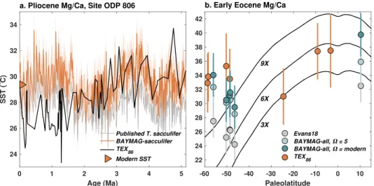
of 5.2 mmol/mol, according to our ensemble estimate. Although this is a small change, it does impact SST prediction, as can been seen from comparison with the published SST estimates (Wara et al., 2005), which use the Dekens et al. (2002) calibration and did not account for changing Mg/Ca_sw(Figure 10a). Whereas the original SST estimates suggest that Pliocene SSTs were consistently cooler than modern, the BAYMAG estimates indicate that they were mostly similar to, or warmer than, modern values and bring the data into better agreement with independent estimates from the TEX86proxy (Zhang et al., 2014) (Figure 10a).

Figure 10. Application of BAYMAG to Cenozoic Mg/Ca data, with correction for changing Mg/Casw. (a) Mg/Ca data

extending back to the Pliocene from Site ODP 806 (Wara et al., 2005). Triangle indicates modern mean annual SST. (b) Mg/Ca data (Hines et al., 2017; Hollis et al., 2009; Hollis et al., 2012; Tripati et al., 2003) from the Early Eocene Climatic Optimum (53.3–49.1 Ma), plotted by paleolatitude. Black lines denote predicted SSTs from Eocene climate model simulations conducted under 3×, 6×, and 9×preindustrial CO₂levels (Zhu et al., 2019). In both panels, TEX₈₆ data (calibrated with BAYSPAR, Tierney & Tingley, 2014) are plotted for comparison. Shading and error bars represent

1𝜎uncertainties.

Next, we apply BAYMAG to Mg/Ca data from the Early Eocene Climatic Optimum (EECO, 53.3–49.1 Ma), one of the warmest times during the Cenozoic Era. These data include Morozovella spp. from site ODP 865 (Tripati et al., 2003), hemipelagic outcrops from the eastern shore of New Zealand (mid-Waipara, Tawanui, Tora, and Hampden Beach, Hollis et al., 2009, 2012; Hines et al., 2017), and DSDP Site 277 (Hines et al., 2017). Morozovella spp. species are extinct, so we do not know their seasonal or depth habitat preferences. Thus, we use the pooled annual model, which provides generic constraints on temperature, salinity, pH, and Ω sensitivities. Following Evans et al. (2018), we assume, based on carbon modeling constraints (Tyrrell & Zeebe, 2004), that ocean pH is approximately 7.7 during the EECO. Since we have no good knowledge of how salinity changed, we hold it constant at a value of 34.5 for each site. For Ω, we test two assumptions: (1) that the foraminifera are essentially pristine, unaltered by seafloor dissolution (Ω = 5), and (2) that the foraminifera have experienced dissolution on par with what we would expect at the site locations today. For this latter assumption, we draw Ω from GLODAPv2 using the paleolatitude and paleolongitude (calculated from Baatsen et al., 2016, as suggested in Hollis et al., 2019) and the inferred Eocene water depth as described in the original publication. We use an uninformative prior standard deviation of 10◦C.

We compare our results to the inferences made by Evans et al. (2018) using the same Mg/Ca data, as well as independent estimates of SST from EECO TEX86data spanning similar paleolatitudes (Bijl et al., 2009;

Bijl et al., 2013; Cramwinckel et al., 2018; Hollis et al., 2009, 2012; Inglis et al., 2015; Pearson et al., 2007) calibrated with BAYSPAR (Hollis et al., 2019; Tierney & Tingley, 2014) (Figure 10b). All of the estimates from BAYMAG are warmer, on average, than those of Evans et al. (2018), by 4.3◦C under the assumption of no dissolution, and by 5.8◦C with modern Ω estimates (Figure 10b). Since our inferred Mg/Caswvalue

for the Eocene (2.2 mmol/mol) is the same as Evans et al. (2018), this difference reflects model form. Evans et al. (2018) first correct Mg/Ca for the pH effect using laboratory constraints (Evans, Wade, et al., 2016) and then calculate SST assuming a reduced temperature sensitivity at lower Mg/Ca_sw, using coefficients derived from G. ruber culture experiments (Evans, Brierley, et al., 2016).

In the absence of information concerning the Eocene carbonate system, Evans et al. (2018) assume no loss from dissolution at depth. For shallow and intermediate-depth sites considered here, allowing some disso-lution increases median SST estimates up by 0.3–1.5◦C—a relatively minor effect. ODP 865 is an exception: Here, using a modern estimate of Ω yields median SST estimates that are 3.9◦C higher. This is because plate rotations (Baatsen et al., 2016; Herold et al., 2014) predict that this site was located much closer to the equa-tor (4–10◦N, vs. 18◦N today) and farther east (138–144◦W, vs. 179◦W today) during the EECO. Today, the