HAL Id: halshs-00261582
https://halshs.archives-ouvertes.fr/halshs-00261582
Submitted on 7 Mar 2008
HAL is a multi-disciplinary open access
archive for the deposit and dissemination of sci-entific research documents, whether they are pub-lished or not. The documents may come from teaching and research institutions in France or abroad, or from public or private research centers.
L’archive ouverte pluridisciplinaire HAL, est destinée au dépôt et à la diffusion de documents scientifiques de niveau recherche, publiés ou non, émanant des établissements d’enseignement et de recherche français ou étrangers, des laboratoires publics ou privés.
The rationality of expectations formation and excess
volatility
Julio Davila
To cite this version:
Documents de Travail du
Centre d’Economie de la Sorbonne
Maison des Sciences Économiques, 106-112 boulevard de L'Hôpital, 75647 Paris Cedex 13 http://ces.univ-paris1.fr/cesdp/CES-docs.htm
The rationality of expectations formation and excess volatility
Julio DAVILA
THE RATIONALITY OF EXPECTATIONS FORMATION AND EXCESS VOLATILITY
Julio D´avila Paris School of Economics
February 2008
Abstract. That dropping the rational expectations assumption opens the door to many more patterns of volatility as equilibrium phenomena is not surprising. That this continues to be so even after requiring the expectations to be formed rationally is indeed surprising. In effect, requiring the agents to form expectations rationally —in the sense of being such that they maximize at any time the likelihood of observed history— does not pin down what is an equilibrium outcome much better than allow-ing for arbitrary expectations, unless the agents have access to unlimited historical records or memory. More specifically, I establish, in simple deterministic overlapping generations economies, that if each agent holds rationally formed expectations in the sense that any other expectations justifying his choices imply a smaller likelihood for the history he observes with limited memory, then there are rationally formed expectations equilibria exhibiting an excess volatility that no rational expectations equilibrium can match. Moreover, from the allocation viewpoint, these new equi-libria can be supported also by many other expectations (not necessarily rationally formed). Given that the limited records or finite memory case may arguably be the relevant one from a positive viewpoint, this result suggests that the possibility of excess volatility as an equilibrium phenomenon has been downplayed by the use of the rational expectations hypothesis.
1. Introduction
Volatility of prices is undesirable for risk averse agents because it prevents them to be certain about the prices they will face in the future, which may lead them to incur in costly mistakes. An important part of the price volatility seems to be an unavoidable consequence of the uncertainty about the fundamentals themselves. But prices usually exhibit a much higher variance than the fundamentals.1 The
variance of prices that cannot be completely justified by that of the fundamentals
I thank helpful comments on an earlier version of this paper from attendants to the 3rd CARESS-Cowles Conference on General Equilibrium and its Applications, the 2007 SAET con-ference, the 2007 European Workshop on General Equilibrium Theory, the 2007 Far Eastern Meeting of the Econometric Society, and to attendants to seminars in the University of Tokyo, Kyoto University, and Kobe University.
1See Shiller (1981) for an account focused on stock prices in particular.
is referred to as excess volatility.2 Given its cost in terms of efficiency and welfare,
it is of obvious interest to have an assessment of to what extent and how excess volatility can be avoided or at least reduced. Of course, first one would like to have an idea of how serious the problem may be according to the best understanding available of how sequential competitive markets work.
Excess volatility has long been thought to be the result of the agents’ own deci-sions as they expect this same volatility to take place.3 This has been so because
there seems to be a self-confirming or self-fulfilling aspect in the nature of excess volatility. Even if this suggests that there must be something irrational about excess volatility, it has nevertheless been shown that the phenomenon of excess volatility is perfectly consistent with the notion of rational expectations equilibrium that is standard for sequential dynamic general equilibrium models, in particular through its sunspot equilibrium version.4 Still, I argue in this paper that the use of the
rational expectations hypothesis may very well underestimate the possibility of ex-cess volatility of prices and trades as an equilibrium outcome. Interestingly enough, this misleading feature of the rational expectations equilibrium notion becomes ap-parent when one tries to address the fact that the rational expectations hypothesis does not provide an expectations formation theory, which turns out to be not as innocuous as it seems from the viewpoint of the rationality of expectations.
In effect, general equilibrium models leave unmodelled the formation of prices as well as the formation of expectations over future prices, whenever markets open se-quentially. The equilibrium equations only impose on prices the condition of being such that markets clear when agents react rationally to them, but no explanation is provided as to how these prices do actually emerge in the market, which is rather inconvenient in the very common case in which there is a multiplicity of equilibria. As for the expectations, they are often required to satisfy a condition that rules out the possibility of the agents making systematic forecasting mistakes that would compromise their assumed rationality. The satisfaction of this condition —namely, the identification of subjective and objective expectations about future prices— is the rational expectations hypothesis. But the corresponding notion of rational expectations equilibrium does not provide any more explanations about how the agents form their expectations about future prices than about the formation of prices themselves. In this sense, the condition imposed by the rational expecta-tions hypothesis is unduely freed from the requirement of having to be consistent with some procedure (hopefully reasonable) that the agents may use to form their expectations.
At least two strands of the literature have addressed the issue of how can the agents get to know the expectations held in a rational expectations equilibrium,
2This term is used in the literature to refer more specifically to the volatility exhibited in
particular by stock prices in excess of what would be justifiable from changes in the present value of future dividends to be distributed by firms, but I’ll use it here to refer, more generally, to that part of the volatility of the prices determined by a general equilibrium model that exceeds the volatility of the fundamentals.
3Shiller (1987) attributes to Pigou (1929) the view that ”psychological causes”, along with
”monetary causes”, can account for as much as a half of the amplitude of aggregate fluctuations.
4See Shell (1977) and Cass and Shell (1983) for the seminal papers on the notion of sunspot
equilibrium, Azariadis (1981) for its first application to the overlapping generations model, and Woodford (1986) for an application to infinitely-lived agents with finance constraints.
namely the adaptive learning and the eductive learning literatures. The adap-tive learning approach5 considers under what conditions the process followed by
prices in a rational expectations equilibrium can be learned, in real time, updating the information available as the process realizes.6 Quite differently, the eductive
learning approach tries to characterize the conditions under which, from the very understanding of the problem they face, the agents can deduce in no time that a particular rational expectations equilibrium is the only possible outcome (at least locally) and hence they coordinate immediately on it.7 Nevertheless, rational
expec-tations equilibria that are not ”learnable” by an updating process (as the adaptive learning literature would like) or rationalizable in a game-theoretic sense (as the eductive learning literature would desire) are not less of an equilibrium than those that are learnable in one way or another. Thus it should be noted from the start that both the adaptive and the eductive learning approaches look essentially for ways to discern whether some rational expectations equilibria are more ”reason-able” than others, i.e. following a logic of refinement of the equilibrium concept. As a matter of fact, these approaches originated from the need to address the in-determinacy problem that the existence of a multiplicity of rational expectations equilibria usually created. Here, I address instead the issue of whether the rational expectations equilibrium concept itself has led to overlooking some excess volatility phenomena as equilibrium outcomes, which leads us to scrutinize the implicit as-sumptions (or rather the lack of them) on the rationality of the process of formation of expectations under the rational expectations hypothesis.
In effect, the lack of implications of the rational expectations hypothesis on an expectations formation theory makes possible that, for instance, the expectations prescribed to an agent at any given date by a rational expectations equilibrium need not be those that explain best the history observed by the agent then. But, since any sensible expectations formation theory should make the agents’ expectations follow from the information available to them at the time of making their decisions —namely the history of past prices— this is a clear shortcoming of the rational expectations hypothesis that does not become apparent until the expectations for-mation issue is addressed.
Also, in a stationary rational expectations equilibrium the agents’ beliefs are history independent, which is clearly counterfactual, unless the agents have access to infinite histories of past prices and unlimited computing ability to process them. From a positive viewpoint, beliefs do result from past experiences —which actually do never extend (or at least their records) to an infinitely remote past— and the de-pendence of actual beliefs on the observed past is also clearly non-trivial. Since any sensible theory about the formation of the agents’ beliefs, and hence expectations, needs to make them follow from the information available to agents at the time they make their decisions, then an alternative assumption about the expectations at equilibrium is needed.
5See for instance Evans and Honkapohja (2001) for a recent account.
6See, for instance, Woodford (1990) and Evans-Honkapohja (2003) for the possibility of learning
this way the expectations of a stationary sunspot equilibrium.
7See Desgranges-Negroni (2003) for the issue of the coordination of expectations on a sunspot
equilibrium through an eductive approach. For the seminal paper on the eductive learning ap-proach see Guesnerie (1992).
Alternatively to the refinement logic, one can think of imposing on the expec-tations other rationality conditions that are compatible with some sensible way of forming expectations from observable data. The need for these rationality condi-tions to comply with some sensible expectacondi-tions formation theory is particularly pressing in the case in which the phenomenon of excess volatility is most dramatic, namely when there is no uncertainty at all about the fundamentals (in the extreme ideal case in which the fundamentals are deterministic, any variance exhibited by prices and trades corresponds, by definition, to excess volatility). In effect, while in the presence of shocks to the fundamentals it is natural to assume that the agents can use the information they may have on the stochastic process followed by these shocks in order to form their beliefs on that process, and hence their expectations about future realizations and prices, when no shock affects the fundamentals the origin of expectations remains a mystery,8 and they look as being pinned down, at
equilibrium, only by their self-confirming character. When one modifies accordingly the equilibrium notion in order to introduce a rationality condition on expectations that is consistent with some sensible way to form expectations, new instances of excess volatility of prices and trades turn out to be equilibrium outcomes.
That new instances of equilibrium excess volatility appear when the expectations are not required to coincide with objective ones (as rational expectations would have it) is not surprising, since many more degrees of freedom are introduced in this way. That the most sensible rationality requirements from the formations of expectations —namely that they are consistent with the information available at the time of their formation— does not constrain what can be and what cannot be an equilibrium excess volatility any more than letting expectations to be arbitrary ones is certainly surprising.
In particular, I explore in this paper the consequences of taking the view that, whenever several distinct beliefs or expectations can lead an agent to make a given decision, to assume that the agent’s beliefs are not those that explain best the ob-served history amounts to assume that the agent does not form his expectations or beliefs rationally, whatever the method used is. As a consequence, I consider the rationality condition on the formation of expectations that requires that when-ever swhen-everal beliefs justify a given choice, the agent is supposed to hold those that conform best with his observations.
One could say that, if the rational expectations hypothesis ”is nothing else than the extension of the rationality hypothesis to expectations” (Guesnerie (1992)), the hypothesis above is nothing else than the extension of the rationality hypothesis to the formation of expectations. Moreover, imposing a rationality condition on the formation of expectations seems more natural than imposing a rationality condi-tion on expectacondi-tions themselves, since the problem of formacondi-tion of expectacondi-tions is in essence a choice problem on which rationality requirements are more straight-forwardly meaningful than the usual rational expectations requirement that the agents ”know the model”, which is only a handwaving substitute for the explicit acknowledgement of the Nash-like, fixed point nature of the rational expectations. Nevertheless, I wish to stress that I do stop short of modelling explicitly the
forma-8In a sunspot equilibrium the beliefs have the logical status of a Nash equilibrium in beliefs,
with the coordination problem that that brings along in the (very common) case in which there is a multiplicity of them.
tion of expectations as a choice problem. I will just require that, however this choice problem may be modelled, the resulting expectations must satisfy the rationality condition expressed above, namely that the expectations or beliefs upon which a decision is made must explain history better than any other beliefs justifying the same decision.
More specifically, I will consider in a deterministic overlapping generations ex-change economy that agents hold rationally formed expectations, in the sense that any other expectations consistent with their choices follow from beliefs implying a smaller likelihood for the history they observe. I show then first that a belief by the agents that the history they observe is Markovian can never be falsified (Lemma 1). Then, restricting the analysis to Markovian beliefs, I establish that whenever the agents’ memories or records of past events are finite (which is the rel-evant positive case), there exist rationally formed expectations equilibria exhibiting an excess volatility that no rational expectations (sunspot) equilibrium can match (Proposition 3). Quite disturbingly, what kind of excess volatility can be an equi-librium outcome is not actually constrained by the rationality condition above on the formation of expectations, the new instances of equilibrium excess volatility be-ing the same as those driven by many other expectations not necessarily rationally formed. Nonetheless, the existence of such equilibria in this abstraction suggests that the role of excess volatility in the working of actual competitive markets may be much more important than what the widespread use of the rational expectations hypothesis may suggest.
In the alternative counterfactual case in which the agents were able to keep track of an infinite history of past prices, then the only rationally formed expectations equilibria turn out to be those that are observationally equivalent to some rational expectations sunspot equilibrium (Proposition 2).
A rationally formed expectations equilibrium will thus consist of, for each agent in each generation and for every history of prices he may observe, (1) a belief that the prices follow a particular stochastic process, and (2) consumption decisions (contingent to future prices in the case of future consumptions), such that, for any history of prices that may realize up to any date, (i) the resulting allocation of resources is feasible, (ii) the agents’ consumption choices maximize their utilities given the price process they believe they face,9and (iii) the agents’ beliefs about the
price process are formed rationally, i.e. their beliefs provide the highest likelihood
to the histories they observe among all the beliefs that could have led them to make the same consumption choices, and are never falsified by the history observed.
Note that the equilibrium concept leaves open the question of how is determined the history of prices that actually realizes. It just requires that it does not falsify the agents’ beliefs. But this does not prevent the agents to believe that prices follow a Markov chain, since this cannot be falsified by any history of prices. In effect, as it will be established in Lemma 1 in Section 3, histories of prices going back into the infinite past exhibit the Markov property, namely that empirical frequencies of transitions between prices depend only on the price from which the transition starts; and for histories of prices with a finite past, any dependence of these empirical frequencies on past prices eventually vanishes.
9For the overlapping generations economies considered below it will turn out that in doing so
Therefore, no objective process is assumed to drive prices. As a consequence, there is no room for agents to mistake a price process they supposedly face (this, in contrast, would be the ultimate rationality test under rational expectations). It is important to stress that, in the absence of shocks to the fundamentals, assuming that some objective stochastic process (like the one followed by a sunspot signal) drives the prices,10 amounts to postulate implicitly a particular price formation
the-ory —extraneous to the equilibrium conditions and hence alien to market-clearing forces— that acts in an ad hoc way as a selecting device within the set of possi-ble price histories. Given the obvious difficulties in justifying the causation from sunspots all the way through prices, I do away with it. Note also that if on the contrary the fundamentals do follow some stochastic process, the latter will make its way through the equilibrium equations towards the equilibrium prices, in such a way that one can safely speak in that case of a stochastic process driving prices. So, the caveat above about assuming an objective price process is truly specific to the pure excess volatility case with deterministic fundamentals that we are considering in this paper.
It will be established below that, in a rationally formed expectations equilibrium of an overlapping generations economy, there is room for different agents (within and across generations) to hold different expectations. This diversity of beliefs across generations is only a natural consequence of the fact that different gener-ations observe different bits of a same history of prices and therefore form their beliefs rationally using different information. Note also that, within generations, the requirement for each agents’ expectations to be consistent with their possi-bly different choices leaves room for the agents to hold different expectations even when they have the same information, which may reflect the very realistic fact of differences of opinion or interpretation even in the face of the same evidence.
In considering explicitly rationality conditions on the way the agents form their beliefs, as part of the definition of the equilibrium, I depart thus from the rational expectations equilibrium concept insofar the latter actually remains silent about how the agents may have arrived to hold such expectations to begin with. The approach followed in this paper thus adds an element missing in the rational ex-pectations equilibrium concept. This will show itself clearly in the definition of a rationally formed expectations equilibrium below, which will embed that of a rational expectations sunspot equilibrium as a rationally formed expectations equi-librium constrained to satisfy the strong and, more importantly, counterfactual requirement of having the agents to hold common beliefs that are independent of the histories they observe.
Before proceeding with the main body of the paper, I will discuss briefly but more specifically the differences between the approach followed in this paper about the rationality in the formation of expectations and some of the approaches in the literature on learning rational expectations. The rationality condition that I consider on the formation of expectations seems reminiscent of the one underlying
10In the sunspot equilibrium literature it is customary to claim that the prices turn out to
be perfectly correlated with the sunspot signal, and hence follow the same process, because the decisions made by the agents according to their belief in such a perfect correlation causes the prices to take the adequate values with the adequate probabilities for that perfect correlation to actually take place. But how the agents’ decisions would achieve this is left unexplained.
the rational beliefs equilibrium concept of Kurz (1994). Nonetheless, rationally formed expectations differ essentially from Kurz’s rational beliefs. They only share the idea that the rationality of expectations or ”beliefs should be defined relative to what is learnable from the data” (Kurz (1994), p.879). Otherwise, Kurz (1994) requires the agents to believe that prices are driven by a process whose long term behavior coincides with that of the true process. Leaving aside the problem posed by the ad hoc character of such a true process in the pure extrinsic uncertainty case, in order to infer such long term behavior Kurz (1994) assumes that the agents have access to infinitely long histories of past prices, a formidable feat that the rationally formed expectations equilibrium does not require.
The approach considered here is also distinct from the adaptive learning approach in Woodford (1990) insofar in that paper the agents learn some information about the ”support” (specifically the optimal labor supply for each value of the sunspot) while I focus on how the agents infer the probabilities of transition between states that have been historically observed. Moreover, in Woodford (1990) agent t’s pref-erences suffer from an additive shock εtst, linear in the agent savings (labor supply
in Woodford’s interpretation), where εt is an independently and identically
dis-tributed process with Et(εt) = 0 and variance σ2> 0 whose distribution the agents
learn from past realizations. It is from the accidental sample correlation between the small fluctuations in the relative price pt
pt+1 generated by these shocks and the
sunspot realizations that agents’ beliefs in the sunspot theory can get reinforced and thus convergence to a stationary sunspot equilibrium obtains. As Woodford points out, the presence of these shocks to the fundamentals is thus essential for the learning to occur. In contrast, in the rationally formed expectations equilibria considered in this paper there is no room for an intrinsic uncertainty to play any role whatsoever.
The remainder of the paper is organized as follows: Section 2 conveys the main ideas by means of a leading example that allows to ”visualize” what is driving the result: it produces constructively rationally formed expectations equilibria ex-hibiting fluctuations distinct from those of any rational expectations equilibrium. Section 3 generalizes the setup, provides a precise definition of a rationally formed expectations equilibrium for a deterministic overlapping generations economy, and establishes the existence of equilibria of this type exhibiting fluctuations that no rational expectations equilibrium could generate. Incidentally, the constructive argument used to establish this result reveals a high level of degrees of freedom to produce rationally formed expectations equilibria. Thus, I conclude establishing next the important fact that not anything can actually be supported as a rationally formed expectations equilibrium.
2. The leading example
2.1 What is a rationally formed expectations equilibrium?
Consider an overlapping generations economy with a 2-period lived representa-tive agent. An agent born in period t lives for two periods and has to make a decision about how much to save from real income y when young (date t) in order to be able to consume when old (date t + 1). His decision will depend on the pur-chasing power he expects his savings to have when old. In particular, if the current
price of consumption is ptand he expects it to be, when old, any of k possible values
pjt+1, for j = 1, . . . , k, with probabilities πj respectively, then his chosen level st of
savings would be determined by the solution to
max k X j=1 πju(ctt, ctjt+1) ct t+ st = y ctjt+1= pt pjt+1s t (1) where ct
t is his consumption when young and ctjt+1 is his consumption when old if
the level of prices then is pjt+1. Under standard assumptions guaranteeing differen-tiability and the interiority of the solution, the necessary and sufficient first-order condition characterizing the solution of the problem above is, along with its budget constraints, k X j=1 πj h − u1(y − st, pt pjt+1s t) + u 2(y − st, pt pjt+1s t) pt pjt+1 i = 0. (2)
At equilibrium every agent must choose his consumption rationally according to his expectations about future prices, and individual consumption decisions must be compatible. Thus in an equilibrium of this economy in which the level of prices takes, at any period, one of k possible values p1, . . . , pk, and the representative
agent believes that the probability πij of the price being pj when old depends then
only on the price pihe faces when young, the representative agent’s savings decision
depends only on the level of prices pihe faces when young, so that it can be denoted
si and be characterized as the solution to k X j=1 πijh− u 1(y − si, p i pjsi) + u2(y − si, pi pjsi) pi pj i = 0. (3)
Moreover, in such an equilibrium the contingent savings si and prices pi, for all
i = 1, . . . , k, satisfy
si = pj
pis
j (4)
for all i, j = 1, . . . , k, so that not only all the agents choose their savings rationally according to their expectations, but markets clear as well (in effect, in any state i the desired saving si by the young agent equals then the desired consumption pj
pisj
by the contemporary old agent born in any state j). Conditions for the existence of prices pi, savings si, and probabilities πij, for i, j = 1, . . . , k, such that (3) and
(4) hold for all i, j = 1, . . . , k are well known,11 and such an equilibrium is known
in the literature as a k-state Markovian stationary sunspot equilibrium.
11See the sunspot equilibrium literature, e.g. Azariadis (1981), Azariadis and Guesnerie (1986),
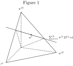
Note however that, as soon as k ≥ 3 in equation (3) the same savings decision
si can follow from different beliefs about the probabilities πi1, . . . , πik of transition
from a price pi to any other pj. In effect, at any such equilibrium each vector
(πi1, . . . , πik) of probabilities of transition from each state i = 1, . . . , k, must satisfy
the two linear equations consisting of (i) being in the unit simplex in Rk and
(ii) satisfying equation (3), so that there remains k − 2 degrees of freedom for each row (πi1, . . . , πik) of the Markov matrix (πij)k
i,j=1 of believed probabilities of
transition between prices, as illustrated in Figure 1 below for the case k = 3, where
πi· ≡ (πi1, . . . , πik) and Dij ≡ −u
1(y − si,p i pjsi) + u2(y − si, p i pjsi)p i pj. Figure 1 ... ... ... ... ... ... ... ... ... ... ... ... ... ... ... ... ... ... ... ... πi3 ...... ... πi2 .... .. .... .. .... .. .... .. .... .. .... .. .... .. .... .. .... .. .... .. .... .. .... .. . πi1 ... ... ... ... ... ... ... ... ... ... ...... ...... .. .. .. .. .. .. .. .. .. .. .. .. .. .. .. .. .. .. .. .. .. .. .. .. .. .. .. .. .. .. .. .. .. .. .. .. .. .. .. P3 j=1πijDij=0 .... .. ... πi· ... ... ... ... ... ... ... ... ... ... ... ... ... ... ... ... ...... ...... ...... ...... ...... ...... ...... ...... .. .. .. .. .. .. .. .. .. .. .. .. .. .. .. .. .. .. .. .. .. .. .. .. .. .. .. .. .. .. .. .. .. .. .. .. .. .. .. .. .. .. .. .. .. .. .. .. .. .. .. .. .. .. .. .. .. .. .. .. .. .. .. .. .. .. .. .. .. .. .. .. .. .. .. .. .. .. .. .. .. .. .. .. .. .. .. .. .. .. .. .. .. .. .. .. .. .. .. .. .. .. .. .. .. .. .. .. .. .. .. .. .. .. .. .. .. .. .. .. .. .. .. .. .. .. .. .. .. .. .. .. .. .. .. .. .. .. .. .. .. .. . ...... ...... ...... ...
Thus equations (3) and (4) may hold true —i.e., (i) everyone behaves rationally
given his believes and (ii) markets clear— even with different agents within and
across generations holding different beliefs about the probabilities of transition πij,
if no further requirement is made on the agents’ beliefs. Of course, this possibility is excluded if the agents are supposed to hold rational expectations, since in that case all the agents must share the same ”true” πij’s. Note however that until now
I have not made any mention to the existence of a ”true” objective process from which this ”true” πij’s would stem, but rather I have only mentioned the agents’
expectations about future prices. That is because in a k-state stationary sunspot equilibrium (and all the corresponding literature) the probability πij with which
the agent expects the transition from a price pi to a price pj to happen is
implic-itly assumed to be the actual probability with which such transition does happen, because of a never falsified belief in a perfect correlation between some sunspot signal and prices.12 Note that this amounts to assuming implicitely a price
forma-tion mechanism that is extraneous to the equilibrium noforma-tion, very much like an ad hoc choice of a particular equilibrium price out of a multiplicity of them in a, for instance, Edgeworth box. More specifically, the rational expectations hypothesis imposes the additional condition that (i) all agents’ expectations coincide, and (ii) that these common expectations correspond to those following from an objective process driving prices. Note that, in terms of the equilibrium equations (3) and (4), this second condition has no bite in the sunspot case, since it can just be dropped
12No explanation of how this correlation happens to appear is usually provided, except for
that of Woodford (1990), and in that case a small seed of uncertainty about the fundamentals is needed for an accidental correlation to get reinforced and convergence to the ”sunspot theory” to obtain.
without any consequence for the set of solutions to the equations. It is in this sense that the assumption of an objective process driving prices is an implicitly ad hoc selection device in the absence of shocks to the fundamentals. But (i) without (ii) becomes arbitrary, and raises difficult questions regarding the spontaneous coordi-nation of every agent within and across the infinity of generations on a particular belief. Accordingly, both (i) and (ii) can arguably be dropped and the relevance of the rational expectations hypothesis be questioned in the absence of shocks to the fundamentals.
As a matter of fact, plenty of beliefs are compatible with the agents’ behavior, and thus there is room for alternative consistency conditions at equilibrium, other than the rational expectations hypothesis, to be imposed on the agents’ expecta-tions, although hopefully only outcomes following from rationally formed beliefs can be equilibrium ones. Moving in this direction, clearly the agents’ expectations should follow from the information available to them at the time of making their decisions. Accordingly, assuming that any given agent’s decision follows from ex-pectations derived from beliefs that do not make the likelihood of the history of prices he observes as big as possible, among all the expectations that would have led to the same decision, is equivalent to assume that the agent formed his expectations irrationally or using inefficiently the available information. In Figure 2 below, for the case k = 3, the agent’s rationally formed expectations about these probabilities of transition from a price pi (if he believes the prices follow a Markov process)
would be the point ¯πi·
tδ (where t stands for the date up to which the generation t
can observe a history of prices δ) attaining the highest likelihood level curve on the unit simplex among those consistent with the first-order condition satisfied by the agent’s saving decision (represented by the plane intersecting the unit simplex in Figure 2). Note that the empirical frequencies of transitions starting from pi (the
number of observed transitions from price pi to each price pj over the number of
times pi has realized, depicted as πi·
tδ in Figure 2) would be the beliefs that best
explain the observed history if no consistency with the agent’s choice is required, but such expectations need not be consistent with the agent’s behavior, or will be so just by chance. Figure 2 ... ... ... ... ... ... ... ... ... ... ... ... ... ... ... ... ... ... ... ... πi3 ...... ... πi2 .... .. .... .. .... .. .... .. .... .. .... .. .... .. .... .. .... .. .... .. .... .. .... .. . πi1 ... ... ... ... ... ... ... ... ... ... ...... ...... .. .. .. .. .. .. .. .. .. .. .. .. .. .. .. .. .. .. .. .. .. .. .. .. .. .. .. .. .. .. .. .. .. .. .. .. .. .. .. P3 j=1πijDij=0 ... ... ... ... ... ....... .... .. ... πi· tδ .... .. ... ¯ πi· tδ ... ... ... ... ... ... ... ... ... ... ... ... ... ... ... ... ...... ...... ...... ...... ...... ...... ...... ...... .. .. .. .. .. .. .. .. .. .. .. .. .. .. .. .. .. .. .. .. .. .. .. .. .. .. .. .. .. .. .. .. .. .. .. .. .. .. .. .. .. .. .. .. .. .. .. .. .. .. .. .. .. .. .. .. .. .. .. .. .. .. .. .. .. .. .. .. .. .. .. .. .. .. .. .. .. .. .. .. .. .. .. .. .. .. .. .. .. .. .. .. .. .. .. .. .. .. .. .. .. .. .. .. .. .. .. .. .. .. .. .. .. .. .. .. .. .. .. .. .. .. .. .. .. .. .. .. .. .. .. .. .. .. .. .. .. .. .. .. .. .. . ...... ...... ...... ...
Thus positive prices ¯pi, savings ¯si, for all i = 1, . . . , k, and history-dependent
beliefs about a markovian price process (¯πtδij)k
up to every date t, such that 3 X j=1 ¯ πijtδ h − u1(y − ¯si,p¯ i ¯ pjs¯i) + u2(y − ¯si, ¯ pi ¯ pjs¯i) ¯ pi ¯ pj i = 0 (5) and ¯ sj = p¯ i ¯ pjs¯ i, ∀j = 1, . . . , k (6)
hold for all i = 1, . . . , k, and for every history δ up to every period t, constitute a rationally formed expectations equilibrium if, and only if, any other vector of probabilities πi·satisfying (5) implies a lower likelihood for the realization of history
δ up to period t than ¯πi·
tδ does, for all i = 1, . . . , k and for every history δ and up
to every period t.
Intuitively, as this example illustrates, at a rationally formed expectations equi-librium the expected probabilities ¯πi·
tδ will typically be different for different
gener-ations, since they will have access to histories of different length or span, and hence the observed empirical frequencies of transition πi·
tδ will be different for different
t’s even for a given history δ. Also, within generations the need for each agent’s
expected probabilities to be consistent with their respective different choices leaves room the agents’ beliefs to differ among them as well.
2.2 Rationally formed expectations equilibria distinct from rational expectations equilibria
From equations (5) and (6) —that differ from those of a sunspot equilibrium only in that they make expectations history dependent— one could be tempted to suspect that any rationally formed expectations equilibrium should converge to a sunspot equilibrium, given that in the case in which an objective sunspot process is supposed to drive prices the empirical frequencies of transition between prices would eventually converge to the actual probabilities of transition. As a consequence, there would not be any allocational difference between the sunspot equilibrium and the rationally formed expectations equilibrium in that case. Nevertheless, this is not exactly so: there do exist rationally formed expectations equilibria whose allocations are not rational expectations equilibrium allocations.
In order to show that rationally formed expectations equilibria do not replicate rational expectation equilibria (in particular from the allocations viewpoint), I will illustrate in this framework the existence of rationally formed expectations equilib-ria fluctuating between some given states even when there is no stationary sunspot equilibrium fluctuating between those states.
The argument is constructive, starting from a k-state Markovian stationary sunspot equilibrium of an overlapping generations economy with a representative agent with utility function u and endowments e = (e1, e2). That is to say, consider,
for all i = 1, . . . , k, a price pi, first and second period consumptions ci
1 and ci2and a
Markov matrix of probabilities of transition (πij)k
i,j=1such that, for all i = 1, . . . , k,
and (ci1, (cj2)kj=1) ∈ arg max k X j=1 πiju(˜ci1, ˜cj2) pi(˜ci1−e1)+pj(˜cj2−e2)=0, ∀j (8)
Then necessarily the contingent consumptions ci
1, ci2 satisfy the equations, for all
i = 1, . . . , k k X j=1 πijDij = 0 (9) where Dij≡ u
1(ci1, cj2)(ci1− e1) + u2(ci1, cj2)(ci2− e2). Figure 1 above shows for k = 3
the linear constraint on the simplex that the equilibrium equations impose on the probabilities of transition from any price pi.
Now imagine this was in fact an economy of two identical (types of) agents A and B per generation, so that u and e are the utility and preferences uh and eh
of both agents h = A, B and, for all i, j = 1, . . . , k, ci
1 and cj2 are the equilibrium
contingent consumptions chi
1 and chj2 of both h = A, B as well. Consider then a
nearby economy in which agent B has a different utility function uB close to u
(while uA continues to be u). Since uB is now different from, but close enough to u
(in values and, at least, first partial derivatives), then the linear constraints on each row of the Markov matrix generated by the first order conditions of agent B still intersect the simplex but differ from those of agents A. Actually, for some robust perturbations the new linear constraints on the probabilities of transition have no intersection with the old ones on the unit simplex, as illustrated in Figure 2 in the case k = 3. Figure 2 ... ... ... ... ... ... ... ... ... ... ... ... ... ... ... ... ... ... ... ... πi3 ...... ... πi2 .... .. .... .. .... .. .... .. .... .. .... .. .... .. .... .. .... .. .... .. .... .. .... .. . πi1 ... ... ... ... ... ... ... ... ... ... ...... ...... .. .. .. .. .. .. .. .. .. .. .. .. .. .. .. .. .. .. .. .. .. .. .. .. .. .. .. .. .. .. .. .. .. .. .. .. .. .. .. C C0 ... ... ... ... ... ... ... ... ... ... ... ... ... ... ... .............. .. .. ... .. . ... .. . ... .. . ... ... .. ... . ... ... ... ... ... ... ... .. . ... .. . .. P3 j=1πijDAij=0 P3 j=1πijDBij=0 ... ... ... ... ... ... ... ... ... ... ... ... ... ... ... ... ...... ...... ...... ...... ...... ...... ...... ...... .. .. .. .. .. .. .. .. .. .. .. .. .. .. .. .. .. .. .. .. .. .. .. .. .. .. .. .. .. .. .. .. .. .. .. .. .. .. .. .. .. .. .. .. .. .. .. .. .. .. .. .. .. .. .. .. .. .. .. .. .. .. .. .. .. .. .. .. .. .. .. .. .. .. .. .. .. .. .. .. .. .. .. .. .. .. .. .. .. .. .. .. .. .. .. .. .. .. .. .. .. .. .. .. .. .. .. .. .. .. .. .. .. .. .. .. .. .. .. .. .. .. .. .. .. .. .. .. .. .. .. .. .. .. .. .. .. .. .. .. .. .. . ...... ...... ...... ... ...... ...... ...... ...... ...
This implies that for the resulting economies there is no Markov matrix that makes
both agents 1 and 2 choose the contingent consumptions ci
1and cj2whenever facing
the prices pi, pj, for all i, j = 1, . . . , k. In effect, as long as the perturbation makes
the normal vector Di·
B to the linear subspace (10) following from for agent B’s
first-order conditions to be distinct from the corresponding vector Di·
A for agent A, but
being spanned by Di·
the system k X j=1 πijDijA = 0 k X j=1 πijDijB = 0 (10)
has no solution within the unit simplex. Note that there is a (k − 2)-dimensional manifold (after normalization) of possible vectors Di·
B satisfying this condition. Of
course, any other perturbation close enough to one on this manifold would still be such that no k-state Markovian stationary sunspot equilibrium exists with this support for the corresponding 2-agent overlapping generations economy.
Notwithstanding, there do exist rationally formed expectations equilibria over the given support for any of the 2-agent economies resulting from such robust perturbations. In effect, for small enough perturbations the unit simplex still has a nonempty intersection with the linear subspaces following from the agents’ first-order conditions and hence, for all h, δ, and t, there exist probabilities (πhijtδ )k
i,j=1,
that maximize the likelihoodQki,j=1(πij)Ptτ =1δτ −1i δτj of observing the history δ up to
period t, among the probabilities of transition in the unit simplex that are consistent with the agent’s first-order conditions
k
X
j=1
πijDijh = 0 (11)
for all i = 1, . . . , k (the existence, illustrated in Figure 3 below for k = 3, is guaranteed by the continuity of the likelihood function and the compactness of the constrained domain). Figure 3 ... ... ... ... ... ... ... ... ... ... ... ... ... ... ... ... ... ... ... ... πi3 ...... ... πi2 .... .. .... .. .... .. .... .. .... .. .... .. .... .. .... .. .... .. .... .. .... .. .... .. . πi1 ... ... ... ... ... ... ... ... ... ... ...... ...... .. .. .. .. .. .. .. .. .. .. .. .. .. .. .. .. .. .. .. .. .. .. .. .. .. .. .. .. .. .. .. .. .. .. .. .. .. .. .. C C0 ... ... ... ... ... ... ... ... ... ... ... ... ... ... ... .............. ... . ... .. . ... ... .. .. .. ... .. . ... .. . ... .. . ... .. . .. ... . .. ... . ... ... .. ... ... ... ... ... ......... P3 j=1πijD ij A=0 P3 j=1πijD ij B=0 .... .. ...π¯tδ2i· .... .. ... ¯ π1i·tδ .... .. ... πi· tδ ... ... ... ... ... ... ... ... ... ... ... ... ... ... ... ...... ...... ...... ...... ...... ...... ...... ...... ...... .. .. .. .. .. .. .. .. .. .. .. .. .. .. .. .. .. .. .. .. .. .. .. .. .. .. .. .. .. .. .. .. .. .. .. .. .. .. .. .. .. .. .. .. .. .. .. .. .. .. .. .. .. .. .. .. .. .. .. .. .. .. .. .. .. .. .. .. .. .. .. .. .. .. .. .. .. .. .. .. .. .. .. .. .. .. .. .. .. .. .. .. .. .. .. .. .. .. .. .. .. .. .. .. .. .. .. .. .. .. .. .. .. .. .. .. .. .. .. .. .. .. .. .. .. .. .. .. .. .. .. .. .. .. .. .. .. .. .. .. .. .. . ...... ...... ...... ... ...... ...... ...... ...... ...
3. The general case
I will formalize entire histories of prices {pt}t∈T (where T can be either N or Z)13
taking at any period any of a finite number14 k of possible values p1, . . . , pk, by
13In the case T = N, a special first generation of agents born old is assumed as usual.
14Prices can be thought of as being expressed in multiples of euro cents, and to be believed
by the agents to be above some sufficiently high value with probability 0, so that prices can take indeed only a finite number (although maybe very big) of values, for all practical purposes.
means of a function δi
t indicating whether the price pi has been realized at period t
or not. Thus δi
t = 1 whenever pt = pi, and equals 0 otherwise. Since only one price
can prevail at any period t, it must hold that Pki=1δi
t = 1 for all t ∈ T . Therefore,
a history of realizations is a sequence δ = {δt}t∈T of k-tuples of k − 1 zeros and one
1 at the position of the realized price at that period, that is to say, for all t ∈ T ,
δt∈ {0, 1}k and
Pk
i=1δti= 1. Let ∆ denote the set of such sequences.
Next I provide a formal definition of a rationally formed expectations equilibrium. Consider a deterministic stationary overlapping generations exchange economy with a representative generation consisting of a number H of 2-period lived agents with utility function uh and endowments eh = (eh
1, eh2), for all h = 1, . . . , H. I will
assume, without loss of generality, that the agents believe that prices follow a k-state Markov chain over k prices (Lemma 1 below establishes that this assumption is not restrictive). Agents have access to historical records of length m (maybe infinity), so that they know the price of the good in the last m periods.
Definition. A rationally formed expectations equilibrium of the deterministic
sta-tionary overlapping generations exchange economy with representative generation
(uh, eh)H
h=1 with memory m consists of
(1) a finite number k of positive prices for consumption, i.e. for each i = 1, . . . , k, some pi > 0,
(2) nonnegative first-period consumptions and contingent plans of second-period
consumptions for each agent at each possible price when young, i.e. for each h = 1, . . . , H and each i = 1, . . . , k, some non-negative (chi
1 , {chj2 }kj=1), and
(3) beliefs about the probabilities of transition between prices for each agent
and any history of prices up to his date of birth, i.e. for all h = 1, . . . , H, all t ∈ T , and all realization δ ∈ ∆, a Markov matrix (πtδhij)k
i,j=1,15
such that
(1) the allocation is feasible, i.e. for all i = 1, . . . , k
H X h=1 (chi1 + chi2 ) = H X h=1 (eh1 + eh2) (12) (2) for every agent h and any history δ up to the date t in which he is born,
his first-period consumption and contingent plan of second-period consump-tions (chi
1 , {chj2 }kj=1) are optimal, given his beliefs, whenever at t the price
is pi, i.e. for all h = 1, . . . , H, all δ ∈ ∆, all t ∈ T , and all i = 1, . . . , k, it
holds ¡ chi1 , {chj2 }kj=1¢= arg max k X j=1 πtδhijuh(ci1, cj2) s.t. pi(ci1− eh1) + pj(cj2− eh2) = 0, ∀j (13)
15Note that although with the chosen notation every agent is supposed to hold beliefs about
the probabilities of transition between prices after every partial history of realizations (i.e. even those beyond his life-span), in fact only the possible histories of realizations up to the date of his decision are relevant for the equilibrium conditions above. If the length m of the memory is finite, then the number of possible bits of history relevant for the agent’s decision is clearly finite, so that every member of every generation is required to hold actually only finitely many beliefs. In the infinite memory case this is still the case if there is a first period, but not any longer if there is no first period, then the number of beliefs would be countable.
(3) for every agent, no other compatible beliefs on the probabilities of transition
(i.e. among those for which his first-period consumption and contingent plan of second-period consumptions (chi
1 , {chj2 }kj=1) are optimal whenever
at t the price is pi) provide a higher likelihood to the history of prices
he remembers, i.e. for all h = 1, . . . , H, all t ∈ N, all δ ∈ ∆,16 and all
i = 1, . . . , k, if πi· ∈ Sk−1 is such that
¡ chi1 , {chj2 }kj=1¢= arg max k X j=1 πijuh(ci1, cj2) s.t. pi(ci 1− eh1) + pj(cj2− eh2) = 0, ∀j (14) then k Y j=1 (πij)Ptτ =t−mδτ −1i δτj ≤ k Y j=1 (πtδhij)Ptτ =t−mδiτ −1δjτ (15) and
(4) the agents beliefs about the probabilities of transition are not falsified by
history, i.e. if m = ∞, then for all h = 1, . . . , H, all t ∈ N, all δ ∈ ∆, and all i, j = 1, . . . , k, πδthij− lim t0→−∞ Pt−1 τ =t0δτiδjτ +1 Pt−1 τ =t0δτi = 0 (16) if T = Z, or lim t→∞ " πhijδt − Pt−1 τ =1δτiδjτ +1 Pt−1 τ =1δτi # = 0 (17)
if T = N, whenever the limit in the left-hand side exists.
Note first that if, in the definition above, the beliefs are constrained to be history and agent independent (so that πδthij becomes πij) and the last conditions (3) and
(4) are dropped, then it becomes the definition of a stationary rational expectations (sunspot) equilibrium following a k-state Markov chain (note that condition (4) is trivially satisfied by a k-SSE). As a consequence, it is worth noticing that, typically, in such a rational expectations equilibrium there exist, for every agent, beliefs about the probabilities of transition that are consistent with his consumption choice but that make the history he observes likelier than the equilibrium beliefs do. Of course the discrepancy of the agents’ believed probabilities of transition with the likelihood maximizing ones after each possible history vanishes in the limit if, as the sunspot equilibrium interpretation would have it, the prices are supposed (as opposed to be believed) to follow actually a given Markov chain. But, as I have argued before, the very existence of a specific stochastic process that drives prices is difficult to justify in the absence of shocks to the fundamentals. Moreover, in the case one wants the equilibrium concept to at least aspire to have some positive content, the
counterfactual assumption that beliefs are history independent points to another weakness of the rational expectations equilibrium concept in this context.
Secondly, note also that the length m of the memory determines, in the last condition of the definition above, the transitions that are remembered by the agent when assessing the likelihood of the recent past according to his beliefs, compared to alternative beliefs. In the case m is infinity, the entire history of prices is re-membered by all generations for these purposes.
Finally note that, as previously claimed, restricting ourselves in the definition above to equilibria in which agents believe that the history of prices has been generated by a Markov process is not really constraining since such a belief cannot be falsified by any history they may observe, as the following lemma establishes. Lemma 1. Any history of prices exhibits, either exactly or asymptotically, the
Markovian property. That is to say, more precisely, for any given history δ = {δt}t∈T ∈ ∆ of prices,
(1) if T = Z, then the sequence of empirical frequencies of transition from any
price pi to a price pj is constant, and
(2) if T = N, then the sequence of empirical frequencies of transition from any
price pi to a price pj converges.
Proof. Assume first that T = N. The difference between two consecutive terms of
the empirical frequency of transitions from any given price pi to a price pj is
Pt τ =1δiτδτ +1j Pt τ =1δτi − Pt−1 τ =1δiτδjτ +1 Pt−1 τ =1δτi = Pt 1 τ =1δiτ Pt−1 τ =1δiτ " t−1 X τ =1 δiτ t X τ =1 δτiδτ +1j − t X τ =1 δiτ t−1 X τ =1 δiτδτ +1j # = Pt 1 τ =1δiτ Pt−1 τ =1δiτ "t−1 X τ =1 δi τ Ã δi tδjt+1+ t−1 X τ =1 δi τδjτ +1 ! − Ã δi t+ t−1 X τ =1 δi τ !t−1 X τ =1 δi τδjτ +1 # = Ptδti τ =1δiτ " δjt+1− Pt−1 τ =1δτiδτ +1j Pt−1 τ =1δiτ # (18) Now only two cases must be considered. Either price pi is visited finitely many
times, or countably many times. If it is visited finitely many times then for some t onwards δi
t = 0, so that the distance between the empirical frequencies of transition
becomes 0 from that term on. Hence the sequence of empirical frequencies of transition from pi to pj becomes constant and therefore convergent. If pi is visited
countably many times, then the first factor of the last expression converges to zero (the numerator is bounded and the denominator is decreasing and not non-increasing), while the second factor between brackets is in the bounded interval [−1, 1] (the first term is in {0, 1} and the second is in [0, 1]), then this sequence of differences converges to zero, and hence so does the distance between empirical frequencies of transition from pi to pj. Since the interval [0, 1], being compact,
is complete, then the empirical frequencies of transition from pi to pj themselves
If T = Z, the empirical frequency at any given date t of the transitions from any price pi to any price pj is the limit
lim t0→−∞ Pt−1 τ =t0δτiδjτ +1 Pt−1 τ =t0δτi (19)
which exists for the same reasons as above (the sequence of empirical frequencies of transitions from pi to pj over a period extending increasingly backwards is Cauchy
in a complete space, the compact [0, 1]) and is independent of t. The constancy of the sequence of empirical frequencies from pi to pj follows then trivially. Q.E.D.
The previous lemma has the following important implications. In the case his-tory extends infinitely into the past and the agents keep records of the entire past history, their belief in the price process being a realization of a Markov chain is never falsified, no matter what sequence of prices is realized. In the alternative case in which history starts at a definite date —so that recorded history consists always of a finite set of observations for each generation— and the agents keep records of the entire finite history at their disposal, they see any dependence of the probabilities of transition on earlier prices having the tendency to vanish, i.e. the Markovian property of the history of prices —and hence the agents’ belief— tends to be confirmed, rather than falsified, as time goes by. The same will be true in both cases if the agents’ memory is finite but long enough to observe the tendency towards convergence of the empirical frequencies of transition. So, whatever is the process that determines the sequence of prices, the possibility that the realized se-quence falsifies the agents’ beliefs that this process is Markovian vanishes for long enough memories.
At any rate, and even more importantly, even in the case the agents do not have access to historical records long enough to see disappearing any dependence of probabilities of transition on past prices, the agents know nonetheless that should they have had access to the entire history, that would have only confirmed their belief that they are facing a Markovian price process. As a consequence, such a belief is utmost rational even when limited records are not long enough to confirm it.
Of course if the memory is finite or T = N the agents will share the belief in Markovian prices while not agreeing on the specific probabilities of transition governing that process, since they have access to different bits of history. On the contrary, if memory is infinite and T = Z, they all have to agree on the probabilities of transitions as well; while, finally, if memory is infinite and T = N, they all ”eventually agree”, meaning that discrepancies of subsequent generations vanish.
In the last two cases, in which all agents agree (maybe asymptotically) on the probabilities of transition as well, the limit of the sequence of empirical frequencies would necessarily have to be in the intersection on the unit simplex of the linear subspaces determined by the agents’ FOCs, as shown in Proposition 2 below. In other words, in case of infinite memory the only rationally formed expectations equilibria are those for which such an intersection exists. But these equilibria are observationally equivalent to the rational expectations sunspot equilibrium associ-ated with such an intersection.
Proposition 2. If m is infinite, any rationally formed expectations equilibrium of
the stationary deterministic overlapping generations exchange economy (uh, eh)H h=1
is observationally equivalent to a k-state Markovian stationary sunspot equilib-rium.
Proof. From Lemma 1 the empirical frequencies of transition between any two prices
converge, for any realization of prices, independently of whether the sequence is a realization of a Markov chain or not.
Assume that at a rationally formed expectations equilibrium the linear subspaces induced by the agents FOCs do not intersect on the unit simplex for transitions from pi. Then the distance from some agent’s beliefs about the probabilities of
transition to the limits of the empirical frequencies remains bounded away from zero, which cannot be at equilibrium because of condition (4) in the definition.
Therefore, in this case at a rationally formed expectations equilibrium the linear subspaces induced by the agents FOCs do intersect on the unit simplex for every price pi at the limit of the empirical transitions, and then the rationally formed
expectations equilibrium is observationally equivalent to the k-state Markovian stationary sunspot equilibrium with a Markov matrix whose entries are precisely these limits of the empirical frequencies of transition. Q.E.D.
Therefore, rationally formed expectations equilibria that are distinct from ratio-nal expectations equilibria in this setup, can only appear in the case in which the memory is finite. There can be many reasons why m is finite in the relevant cases. People tend to make forecasts based on their recent experiences, with memories of variable lengths, but certainly of finite length if only because of their actual and unavoidable limited recording and computing capacity. Thus the limited memory case seems to be the relevant one for addressing observed excess volatilities, while the observational equivalence of rationally formed expectations equilibria and ra-tional expectations sunspot equilibria in the infinite memory case makes rather an interesting point as limiting theoretical result.
The next proposition establishes that any deterministic stationary overlapping generations economy with sunspot equilibria can be perturbed robustly in order to produce rationally formed expectations equilibria that no sunspot equilibrium can match. Therefore the use of the rational expectations hypothesis discards all the excess volatility exhibited by these equilibria and, in this sense, downplays the role that expectations have in the fluctuations of the economy.
Proposition 3. Arbitrarily close17 to every deterministic stationary overlapping
generations economy with a finite-state Markovian stationary sunspot equilibrium there exists an economy with finite-memory rationally formed expectations equilib-ria distinct from any sunspot equilibrium.
Proof. Let (uh, eh)H
h=1 be the representative generation of a stationary overlapping
generations economy, and let ©pi, chi
1 , chi2
ªi=k,h=H
i=1,h=1 be the contingent prices and
consumptions of a k-state Markovian stationary sunspot equilibrium of the economy driven by a Markov chain with matrix of probabilities of transition (πij)k
i,j=1.
Assume, without loss of generality, that the allocation corresponding in this equilibrium to the agents of type H only is feasible with their only resources, i.e.18
cHi1 + cHi2 = eH1 + eH2 . (20) Consider a new economy with a representative generation (uh, eh)H+1
h=1 consisting
of adding an agent H + 1 with the same endowments and consumptions as agent
H (the new allocation of the new economy is feasible because of the assumption
above), and a utility function uH+1 with gradients at the consumption bundles
(cHi
1 , cHj2 )ki,j=1 such that, for some i = 1, . . . , k, the vector (Dui1H+1, . . . , DikuH+1),
where Duijh ≡ uh1(chi1 , c
hj
2 )(chi1 − eh1) + uh2(chi1 , chj2 )(chj2 − eh2) for h = H + 1, is both
not collinear to (Di1
uH, . . . , DikuH) and in the span of this vector and (1, . . . , 1), i.e.
Di1 uH+1 .. . Dik uH+1 = α Di1 uH .. . Dik uH + β 1 .. . 1 (21)
for some α and β, with β 6= 0.19 Then the system of equations in the probabilities
πij
πi1Di1
uH+ · · · + πikDikuH = 0
πi1Di1uH+1+ · · · + πikDuikH+1 = 0.
(22)
has no solution. In effect, using the equation (21) above, the second equation can be written equivalently as
α¡πi1Di1uH + · · · + πikDikuH
¢
+ β(πi1+ · · · + πik) = 0 (23) but since Pkj=1πijDij
uH = 0 and β 6= 0, then one would have to have that
πi1+ · · · + πik = 0!! (24) This establishes that the prices and consumptions ©pi, chi
1 , chi2
ªi=k,h=H+1
i=1,h=1 , with
(cH+1i1 , cH+1j2 )k
i,j=1 = (cHi1 , cHj2 )ki,j=1, are not those of a sunspot equilibrium of
the economy with representative generation (uh, eh)H+1
h=1 (in effect, otherwise the
system above would have a solution). They nevertheless are the allocation and prices of a rationally formed expectations equilibrium of this economy.
In effect, if uH+1 is close enough to uH in the topology of C1-convergence over
compacta, then for all h = 1, . . . , H + 1, all t ∈ N, and all δ ∈ ∆, there exists ¡
πhijtδ ¢ki,j=1 satisfying ¡
πtδhij¢ki,j=1= arg max
πij k Y i,j=1 (πij)Ptτ =t−mδτ −1i δjτ s.t. ∀i, πi·∈Sk−1 ∀i,¡chi 1 ,{c hj 2 }kj=1 ¢ =arg maxPk j=1πijuh(ci1,c j 2) s.t. pi(ci 1−eh1)+pj(cj2−eh2)=0, ∀j (25)
18There is always a subset of types of agents for which this is true (note that this subset needs
not be proper). In general, the replication and perturbation argument would then be done on all the types of agents of the subset.
19Note that since Pk
j=1πijDijuH = 0, the vector (Dui1H, . . . , DuikH) cannot be collinear to
(1, . . . , 1). Moreover there is a 1-dimensional manifold of directions that the vector (Di1
uH+1, . . . ,
Dik