The power of some standard tests of stationarity against changes in the unconditional variance

HAL Id: halshs-00476024

https://halshs.archives-ouvertes.fr/halshs-00476024

Submitted on 23 Apr 2010

HAL is a multi-disciplinary open access

archive for the deposit and dissemination of

sci-entific research documents, whether they are

pub-lished or not. The documents may come from

teaching and research institutions in France or

abroad, or from public or private research centers.

L’archive ouverte pluridisciplinaire HAL, est

destinée au dépôt et à la diffusion de documents

scientifiques de niveau recherche, publiés ou non,

émanant des établissements d’enseignement et de

recherche français ou étrangers, des laboratoires

publics ou privés.

The power of some standard tests of stationarity against

changes in the unconditional variance

Ibrahim Ahamada, Mohamed Boutahar

To cite this version:

Ibrahim Ahamada, Mohamed Boutahar. The power of some standard tests of stationarity against

changes in the unconditional variance. 2010. �halshs-00476024�

Documents de Travail du

Centre d’Economie de la Sorbonne

The Power of some Standard tests of stationarity against

changes in the unconditional variance

Ibrahim A

Mohamed B

2010.28

The Power of some Standard tests of stationarity against changes

in the unconditional variance.

Ibrahim AHAMADA

University of Paris 1.

106-112 bd de l’Hôpital 75013 Paris,France.

Tel: (33)0144078208. Mel: ahamada@univ-paris1.fr

Mohamed BOUTAHAR

University of Aix-Marseille II.

2 Rue de la charité Marseille,France.

Mel: boutahar@univmed.fr

April 3, 2010

Abstract

Abrupt changes in the unconditional variance of returns have been recently revealed in many empirical studies. In this paper, we show that traditional KPSS-based tests have a low power against nonstationar-ities stemming from changes in the unconditional variance. More precisely we show that even under very strong abrupt changes in the unconditional variance, the asymptotic moments of the statistics of these tests remain unchanged. To overcome this problem, we use some CUSUM-based tests adapted for small samples. These tests do not compete with KPSS-based tests and can be considered as complementary. CUSUM-based tests con…rm the presence of strong abrupt changes in the unconditional variance of stock returns, whereas KPSS-based tests do not. Consequently, traditional stationary models are not always appropriate to describe stock returns. Finally we show how a model allowing abrupt changes in the unconditional variance is well appropriate for CAC 40 stock returns.

Keywords: KPSS test, Panel stationarity test, Unconditional variance, Abrupt changes, Stock returns, Size-Power curve.

JEL classi…cation: C12; C15; C23.

Résumé

Dans ce papier nous montrons dans un premier temps que les moments asymptotiques des statistiques du test KPSS et ses extensions en panel restent inchangés aux variations brusques de la variance inconditionnelle même si l’ampleur du saut reste élevé. Dans un deuxième temps nous étudions des tests complémentaires ainsi que leurs propriétés asymptotiques. Les tests complémentaires s’adaptent bien aux échantillons réduits puisque nous donnons aussi des valeurs simulées des moments des statistiques en fonction de T, nombre des observations. En…n une illustration concrète est proposée à partir de la série SP500.

Mots-clés: Test KPSS, Tests de stationnarité en panel, Variance inconditionnelle, Changements brusques, Rendements …nanciers, Courbe Taille-Puissance

1

Introduction

Many popular econometric models assume that observations come from covariance-stationary processes. The KPSS test (Kwiatkowski, Phillips, Schmidt and Shin (1992)) is often used to test the null hypothesis of stationarity against its alternative of unit root. This test has become popular and it is systematically implemented by many commercial software programs (thus increasing its usage). Extensions of this test for heterogeneous panel data are developed by Hadri (2000). The null hypothesis of Hadri’s approach is the stationarity in all units (i.e., all individual time series) against the alternative of unit root in all units. Hadri and Larsson (2005) extended the Hadri test by determining exactly the …rst and the second moment of the test statistics when the time dimension of the panel is …xed. Asymptotically, the moments of Hadri test statistics and those of Hadri and Larsson (HL test) coincide. The HL test is concerned by the null of stationarity in all units against the alternative of unit root for some units (i.e. the HL test allows some of the individual series to be stationary under the alternative). All these tests are residual-based LM tests. These tests are among the so called …rst generation tests that are designed for cross-sectionally independent panels. Many authors have investigated the performance of these tests (see for example HIouskova and Wagner (2006)).

But this paper focuses essentially on the behavior of the HL test and the KPSS test against a particular form of nonstationarity which is the one explained by abrupt changes in the unconditional variance of the processes. Because the null hypothesis of these tests is stationarity, many practitioners conclude unambiguously that the data come from a covariance-stationary process when the null is not rejected. The …rst aim of this paper is to show that this conclusion is hasty. We show that even under very strong abrupt changes in the unconditional variance, the asymptotic moments of the statistics of these tests remain unchanged. The null is not rejected while the process is not really covariance stationary (since the variance is not constant). Hence a stationary model can be wrongly applied to the data if the null is not rejected. Among many authors, Starica and Granger (2005) noted that some stylized facts of …nancial returns data can be explained by jumps in the unconditional variance. So, traditional stationary models (stationary GARCH model, stationary long-memory model,etc..) are not always appropriate. Starica and Granger (2005) proposed a nonstationary model that takes into account the jumps in the unconditional variance of …nancial returns data. The second

aim of this paper is to examine some possible complementary tests of stationarity that would be able to detect abrupt changes in the unconditional variance. These complementary tests are based on the cumulative sums of squares of residuals (CUSUM) and have a Kolmogorov-Smirnov limiting distribution under the null. A Monte Carlo study shows that the power of the CUSUM-based tests increases with the size of the jumps in the unconditional variance. Moreover, as in the HL test case, the CUSUM-based test for panel data is also appropriate for small samples. These CUSUM-based tests do not compete with the KPSS test and the HL test but they can be used as complementary tests that are able to detect other forms of nonstationarity while other tests cannot. An illustration based on French stock returns (CAC40 index) consolidates the nonstationary model proposed by Starica and Granger (2005). This paper is organized as follows: the second section investigates the behaviour of the KPSS test and HL test against changes in the unconditional variance. In Section Three we describe the CUSUM-based tests (complementary tests) and their asymptotic properties. In Section Four an empirical illustration is proposed before the conclusion of the paper in the last section. Proofs are given in the Appendix.

2

The Power of the KPSS test and the HL test against changes

in unconditional variance.

2.1

Presentation of the KPSS test and the HL test.

In this section we brie‡y describe the KPSS test and the HL test before analysing their abilities to detect nonstationarity explained by changes in unconditional variance.

Let us consider the following process:

yt= rt+ "t t = 1; :::; T (1)

where rt = rt 1 + ut is a random walk and "t is a zero mean stationary process with E(ut"t0 ) = 0;

E(u2

t) = 2u > 0 and E("2t) = "2 > 0. The null hypothesis is H0 : E(u2t) = 2u = 0, which means that

the component rt = r0 is a constant instead of unit root. Under the null hypothesis, yt is stationary

stationarity around r0 is given by: b = T 2PT t=1 S2 t b2 (2) where St= t P j=1be j, b2= _T1 T P t=1be 2

t andbet’s are the residuals from regression yt= r0+ "t. If "t is not a white

noise, a long run variance can be estimated by using non parametric approach. Under the null the statistic b is asymptotically distributed as

Z 1 0

V1(r)2dr where V1(r) = W (r) rW (1) is a standard Brownian

bridge where critical values are simulated. According to Hadri (2000) and Hadri and Larsson (2005), the asymptotic moments of _{b under the null are known, i.e.,}

lim

T!1E(b ) =

1

6 and Tlim!1var(b ) =

1 45:

The HL stationarity test is an extension of the KPSS test. Let us consider the following model:

yit= rit+ "it i = 1; :::; N and t = 1; :::; T (3)

where rit= rit 1+ uit is a random walk and "it is a stationary process with the following conditions: The

"it’s and uit’s are gaussian and i:i:d across i and over t with E("it) = 0; var("it) = 2"i, E(uit) = 0 and

var(uit) = 2ui > 0. The null hypothesis is H0 : E(u2it) = 2ui = 0, 8i = 1; :::; N which means that each

component ritis a constant instead of a unit root. Under the null hypothesis, each individual times series is

stationary around constant ri0. The alternative hypothesis is given by, H1: 2ui > 0 for i = 1; :::; N1 where

N1 N . So, the alternative of the HL test allows some individual units to be stationary while for the Hadri

test (2000) all individual times series are nonstationary under the alternative hypothesis. The statistic of the HL test for stationarity around ri0 is given by:

Z N T = 1 p N N X i=1 b iT T T (4) where for each …xed value of i, the statistic_{b iT} is computed as_{b in equation (2). Under the null, the …rst} and second moments of_{b iT} are precisely given by _T = E(_{b iT}) = T +1_6T (i.e., the asymptotic mean is 1=6) and 2T = var(b iT) = 2T

2

5T +2

90T2 (i.e., the asymptotic variance is 1=45). Hence the HL test is particularly

attractive since it uses exact moments for any …xed value of T while the Hadri test (2000) uses asymptotic moments. From the Lindeberg-Levy central limit theorem, the limiting distribution of Z N T when N ! 1

2.2

The Power of the HL test and the KPSS test against abrupt changes in the

unconditional variance.

In this section we investigate the respective powers of the HL test and the KPSS test against the alternative of nonstationarity explained by changes in unconditional variance. Let us consider the following nonstationary process:

Yit= ri0+ hit"it, i = 1; :::; N ; t = 1; :::; T . (5)

where for each …xed value of i, the sequence (hit) is a bounded deterministic sequence and "it i:i:d(0; 2"i).

The variance of process fYitg is given by var(Yit) = 2"ihit2. Hence if hit is a deterministic step function

then there are abrupt changes in the unconditional variance of the process Yit.

Let mT = E(b iT); 2T = var(b iT) the moments ofb iT if it is computed by using process (5). Then we

have the following:

Theorem:1. Assume in model (5) that for each …xed value of i the sequence (hit) is a bounded

deterministic sequence with the following condition: 1 T T X t=1 h2_{it! h}2_{i2 as T ! 1} (i) Then Z N T = 1 p N N X i=1 b iT mT T !L N (0; 1), (j) lim T!1mT = 1 6 (jj) and lim T!1 2 T = 1 45: (jjj)

Proof: See Appendix.

Theorem 1 shows that the asymptotic mean and variance of the statistic _{b iT} remain unchanged while process (5) is not really covariance stationary. The condition (i) is obviously satis…ed if the hit’s are step

unconditional variance abrupt changes are the same as under the null of covariance-stationarity. Let us now consider the Monte Carlo experiments based on a Data Generating Process according to equation(5), which we denote by DGPH1. We suppose that the hit’s are step functions for i = 1; :::; N0. More precisely

for i = 1; :::; N0, hit = i;j+1 > 0 if t = Ti;j 1+ 1; :::; Ti;j; Ti;j = [ i;jT ]; 0 < i;1 < ::: < i;m < 1 where i;j6= i;k. There are abrupt changes in the unconditional variances of some individual times series and the

dates of changes are given by the Ti;j’s. According to Starica and Granger (2005), the stylized facts of the

SP500 returns data can be explained by this form of nonstationarity instead of the traditional stationary models. For simplicity we take m = 1; i1= 1 and i2= 2 for i = 1; :::; N0. The ratio = 2₁ gives the

size of the jumps in the unconditional variance while N0denotes the number of the individual nonstationary

processes (n0 = N0=N is the proportion of the nonstationary processes). The "it’s are generated from

the standard N (0; 1). Fixed e¤ects ri0 are coming from the uniform distribution U [0; 1]. Table 1 gives

the rejection frequencies of the null hypothesis by using many values of (n0; ) at 5% level of signi…cance.

The values of N and T are …xed to N = 100 and T = 100. We can see that, when n0 increases, the

rejection frequencies of the null hypothesis always remain near the nominal size = 0:05. This also remains true when increasing the size of the jumps in the unconditional variances (i.e. when increasing = 2

1).

Hence, we can conclude that under nonstationarity explained by jumps in the unconditional variances (even for very high jumps,i.e., = 20), the statistic Z N T seems to have the same behavior as under the null

hypothesis of stationarity although the process is not covariance stationary. The HL test seriously fails to detect abrupt changes in the unconditional variance. So, rejection of the null hypothesis by the HL test must be accompanied by a complementary test to take into account possible abrupt changes in the unconditional variance.In table 1, results about KPSS statistic are obtained by taking N = N0= 1.

3

Some complementary tests.

3.1

De…nition

Let us consider model (1) and suppose that the null is true, i.e., rt = r0 for t = 1; :::; N . According to

of process can be hidden as follows:

yt= r0+ ht"t, t = 1; :::; T , (6)

where the htis supposed to be a step deterministic function and "ta covariance stationary process. Without

loss of generality we can always consider in (6) that var("t) = 2 = 1 and thus var(yt) = h2t. It is thus

necessary to use a complementary test to make sure that htis constant. For this, we extend the test suggested

by Inclan and Tiao (1994) to model (6) and to panel data. We focus on the following null hypothesis H0: ht= h in (6).

Let us consider the statistic

T = max t=1;:::;T r T 2 jDtj ; (7) where Dt=_CC_Tt _Tt , Ck = k P j=1be 2

j and bet are the residuals from (6).

Assumption.1: In (6), ("t) is assumed to be i:i:d:N (0; 1).

Theorem:2: Under the null hypothesis and Assumption 1, we have the following results:

i) The limiting distribution of T is given by the one of W0= supr(jW (r)j) where W (r) is a Brownian

Bridge,

ii) P r( ₁< a) = F (a) = 1 2P1_k=1( 1)k+1exp( 2k2a2), iii) The …rst moment of ₁ is given by: E( ₁) = ln(2)p₂ = ,

iv)The centered second moment of ₁ is given by: var( ₁) = ₂[₆ (log(2))2_{] =} 2_.

The statistic T given by (7) is de…ned with the max(.) function, i.e. the Kolmogorov-Smirnov distance.

It allows us to evaluate if the maximal size of the jumps in the unconditional variance is signi…cant. The theorem allows us to know exactly the asymptotic critical values of ₁. From (ii) of Theorem.2, we have F (1:36) t 0:95. So, the critical value at level = 0:05 is C0:05 t 1:36.

extended to the panel model

yit= ri0+ hit"it , i = 1; :::; N , t = 1; :::; T , (8)

where the hit’s are supposed to be deterministic functions and hit> 0.

Assumption 2: ("it) and (uit) are gaussian and i:i:d across i and over t with E("it) = 0; var("it) = 2"i,

E(uit) = 0 and var(uit) = 2ui > 0.

We consider the same assumptions as in the HL test. The initial values ri0’s are treated as …xed unknown

values playing the role of heterogeneous intercepts under the null hypothesis of stationarity. We are concerned by the following null hypothesis:

H0: hit= hi; 8i = 1; :::; N in (8)

against the alternative that the hit’s are not constants for some i = i2; :::; N2 where N2 N . Now we

de…ne the statistic for cross-sectional data as follows: K = _p1 N N X i=1 iT (9) where iT is constructed as in (7) for each …xed i = 1; :::; N .

CorollaryUnder the null hypothesis and Assumption 2, the limiting distribution of K is a standard normal, N (0; 1), as T ! 1 and N ! 1.

The statistic K given by (9) is more appropriate for the asymptotic case i.e. high values of N and T . For low values of T , we can see in Table 2 that the simulated values of E( iT) and var( iT) deviate signi…cantly

from the asymptotic values given by Theorem 2 (i.e. and ). So, a test based on statistic K can be seriously biased for low values of T . As in the case of the HL test, we adapt the statistic K for …nite values of T to improve the …nite sample properties of the test (see also Harris and Tzavalis, 1999). So, the statistic K can be corrected as follows:

K _T T = 1 p N N X i=1 iT T T (10)

where _T and _T are respectively simulated values of E( iT) and [var( iT)]1=2. It is easy to see that from

the Lindeberg-Levy central limit theorem, the statistic K _T T is distributed as N (0; 1) when N ! 1,

under the null hypothesis and Assumption 2. Assumption 2 guarantees the independence of the individual statistics iT. Some values of T and T are given in Table 2. The values of T and T are respectively

obtained by taking the average and the empirical standard deviation of 10:000 replications of the statistic

T given by (7) for each …xed value of T . The numerical values of the statistic T are obtained by using

the following DGP: yt= + "t, t = 1; :::; T , "t N(0; 1). For each replication of T, the constant value

is coming from the uniform distribution in U (0; 5).

3.2

The Power and size of the complementary tests.

3.2.1 Power and size of the test based on the statistic T.

To investigate the power of the complementary test based on the statistic T given by (7) against abrupt

changes in the unconditional variances, we again consider the DGPH1 given by yt= r0+ ht"t , t = 1; :::; T

where ht= I(1 t t ) + I(t + 1 t T ), I(:) equals one if its argument is true and zero otherwise, and

"t i:i:N (0; 1). Parameter can be regarded as the amplitude of the jump of ht whereas t is the break

date. For each replication of DGPH1the parameter r0is generated from the uniform distribution U [0; 1] and

the break date is chosen as t = [ T ] where U [0:1; 0:9]. Rejection frequencies are based on NR= 10000

replications generated from the DGPH1 and the nominal signi…cance level = 0:05. Table 3 shows the

results for many …xed values of . We can observe that the power of the test increases with the amplitude of the variance change and the size T of the data. The size of the test corresponds to = 1 since in this case the process is covariance stationary. The empirical size becomes closer to the nominal size as sample size T increases. It seems that there is no size distortion. Thus this test can be used as a complementary test of the KPSS test against breaks in the unconditional variance.

3.2.2 Power of the test based on the statistic K _T T.

Another way to examine the power of a test can be based on the size-power curve of the test statistic (see Davidson and Mackinnon(1998)). According to the authors, these graphs convey much more information

and in a more easily assimilated form than classical tables do. In this section we investigate the power of the test based on the statistic K _T T by using some size-power curves. This method is especially convenient

when the theoretical distribution of the studied statistic is not complicated to implement. This is the case for statistic K _T T, since its distribution is the standard N (0; 1). A size-power curve is constructed as

follows. Let us consider a statistic having asymptotic distribution function F under the null. Let us denote by f jgNj=1R, NR realizations of the statistic that are obtained by using a DGP which satis…es the

null hypothesis (DGPH0). The P-value of each j is de…ned as follows : pj = 1 F ( j) = Pr( > j). Let

us now consider bF0, the empirical distribution function of fpjgNj=1R de…ned in (0,1) as follows:

b F0(xi) = 1 NR NR X j=1 I(pj xi): (11)

Davidson and MacKinnon(1998) suggest the following choice of fxigmi=1:

xi = 0:001; 0:002; :::; 0:010; 0:015; :::; 0:990; 0:991; :::; 0:999 (m = 215): (12)

Let us now consider bF1 constructed in the same way as bF0 but instead of j we now use NR realizations,

f 0

jgNj=1R, generated by using a DGP which satis…es the alternative hypothesis. The size-power curve of the

statistic is the locus of points ( bF0(xi); bF1(xi)) when xi describes the (0; 1) interval. Let us consider two

alternative hypotheses H₁(a) and H₁(b) for the statistic . If the test based on is more powerful against H₁(a) than against H₁(b) then the size-power curve constructed using a DGP coming from H₁(a) (DGP_H(a)

1 )

converges more quickly to the horizontal line y = 1 than the size-power curve constructed with a DGP coming from H₁(b)(DGP_H(b)

1 ). For more details about the concept of the size-power curve, see Davidson and

Mackinnon (1998).

Now, we use the concept of the size-power curve to study the ability of statistic K _T T to detect abrupt

changes in the unconditional variances. The DGP_H(a) 1

is constructed as follows: yit= ri0+ hit"it where the

hit’s are step functions with amplitude = 2 for i = 1; :::; N0and hit= hi=constant for i = N0+ 1; :::; N .

The quantity n0= N0=N gives the proportion of individual nonstationary time series in the panel. We set

n0 = N0=N for the experiment. The DGP_H(b)

1 is constructed as DGPH (a)

1 but with = 5. Our aim is to

show that the power of the test increases with . The DGPH0 is constructed as follows: yt= ri0+ "it. For

i, the dimensions of the panel are set to (N; T ) = (100; 100) and the number of replications is NR= 10000.

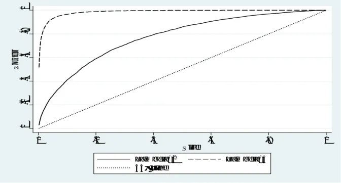
Figure 1 shows the size-power curves. We can see that the size-power curve constructed by using the DGP_H(b)

1 (i.e. with = 5) converges faster to the horizontal line y = 1 than that of the DGPH (a)

1 (i.e. with

= 2). The power of the test increases with the amplitude of the variance break. For comparison purposes, we present in Figure 2 the size-power curves of the HL test statistic by using the same DGP’s. In contrast with the case of statistic K _{T T}, we can now see that the two curves coincide with the 45 line, even for strong abrupt change ( = 5). Thus for the HL test, there is no contrast between the DGPH0 and the two

nonstationary DGP’s, i.e., DGP_H(a) 1

and DGP_H(b) 1

. So the statistic K _T T can be used as a complementary

test of the HL test. Monte Carlo experiments based on many values of ( ; n0; N; T ) were also realized. The

results showed that the power of K _T T increases with and n0. We do not present the results to save

space but they are available on request.

3.2.3 Size of the test based on the statistic K _T T.

Another approach to investigate the sizes of the statistics is the one based on the so called "P-value discrepancy plot" (for more details see Davidson and Mackinnon (1998)). This is simply the graph of

b

F0(xi) xi against xi where bF0 is given by (11). We consider again the stationary DGPH0 presented in

section 3.2.2. If the distribution of the studied statistic is correct, then the pj’s (de…ned in Section 3.2.2)

should be distributed as uniform in (0; 1). Therefore, when bF0(xi) xiis plotted against xi, the graph should

be close to the horizontal axis y = 0. Figure 3 shows the P-value discrepancy plots for the statistic K _T T

and the one for the HL test statistic. We can notice the proximity of both curves with the horizontal line y = 0(values of discrepancies are approximately under 0.01) especially in the case of the statistic K _T T(i.e.

the complementary test). So, there is no size distortion for the two tests. Let us note that in the case of K _T T the curve is nearer to the y = 0 line than in the case of the HL test statistic. Hence, the size of

K _T T seems to be slightly better than in the HL test. Monte Carlo experiments based on many values of

(N; T ) were also performed. The results con…rmed comparable behaviors for the two tests especially in the case of low values of (N; T ). We do not present the results to save space but they are available on request.

4

Empirical illustration.

There has been a long debate about the modeling of the stylized facts of daily stock returns. The absolute returns data often show a slow decay of the sample’s autocorrelation function. Starica and Granger (2005) addressed the following fundamental questions about the persistence of the sample autocorrelation function of stock returns : "How should we interpret the slow decay of the sample autocorrelation function(ACF) of absolute returns? Should we take it at face value, supposing that events that happened a number of years ago have an e¤ect on the present dynamics of returns? Or are the nonstationarities in the returns responsible for its presence?". This question summarizes the classical debate about the modeling of the stock returns. Indeed, the long memory stationary model is often used by many authors to describe the behavior of the sample correlation function of stock returns. Other authors adopt the nonstationary models explained by abrupt changes in the unconditional variance to explain these stylized facts. For an illustration we consider the data of the French …nancial index (CAC40) in logarithm, fln(indexcact)g and returns

f ln(indexcac_{t)g(Figure 4). We consider daily data from January 1, 2003 to January 1, 2004 (the} sample size sample T = 260). Table 4 indicates the results of the KPSS test and the complementary test based on the statistic T. We can see that both tests reject the null of stationarity for ln(indexcact) ( the

critical value for the KPSS test is C0:05 = 0:463 and the one for T is C0:05 = 1:36 ). Then application of

the …lter is often used by many practitioners hoping to obtain covariance stationary data. We can see that the KPSS test does not allow us to reject the null and one can conclude wrongly that ln(indexcact)

is covariance stationary. This conclusion allows us to use some traditional stationary models to describe ln(indexcact) (stationary GARCH model, stationary long-memory model, etc). However, as indicated by

the complementary test ( T), the covariance stationarity of ln(indexcact) is doubtful. The value taken

by T for ln(indexcact) (i.e. T = 3:7669207) remains twice as large as the critical value (C0:05= 1:36).

This result is more compatible with the following model

ln(indexcac_t) = r0+ ht"t (13)

where "t is the covariance stationary process. ht is a step function representing the multiple changes in

the unconditional standard deviation of ln(indexcac_t) . This is exactly the nonstationary model retained by Starica and Granger (2005) for the SP500 stock returns. They found that the forecasts based on this

nonstationary model were superior to those obtained in the framework of stationary GARCH models. They found also that this model reproduces the classical stylized facts observed in returns.

We also consider panel data fln(cacitg, i = 1; :::; N; t = 1; :::; T where cacit is the quotation of the …rms i

which make up the CAC40 index. We consider daily data from January 1, 2003 to January 1, 2004 (N = 40 and T = 260). Table 4 shows that the two tests reject the null of stationarity for ln(cacit) (the critical value

of the two tests is C0:05 = 1:96) while only the statistic K T T indicates abrupt changes in variance. This

result conforms the preceding remarks about the KPSS-test and the statistic T .

4.1

Estimating

h

Starica and Granger (2005) developed an approach based on the stability of the spectral density to compute an estimate of ht(see also Ahamada et al. 2004). Inclan and Tiao (1994) used an iterative algorithm based

on statistic T to estimate ht. Another method allowing us to compute bhteasily and e¤ectively is to apply

the Bai and Perron (2003) approach to the centered data ( ln(indexcact) br0) wherebr0the empirical mean

of ln(indexcact)(we foundrb0= 0:000423). According to (13) one can consider the following regression

with multiple breaks:

yt= k+ vt (14)

where yt= ln(j ln(indexcact) rb0j), k = ln(jhkj) if t = tk 1; :::; tk , the set ftk; k = 1; :::; mg gives the

dates of breaks in the unconditional variance. More precisely these breaks occur in the logarithm of the unconditional standard deviation, i.e. ln(ht): Bai and Perron (2003) addressed the problem of estimation of

the break dates tk and presented an e¢ cient algorithm to obtain global minimizers of the sum of squared

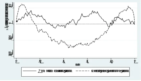
residuals. The algorithm is based on the principle of dynamic programming. They addressed the issue of testing for structural changes under very general conditions on the errors. The issue of estimating the number of breaks m is also considered by the authors. From the Bai and Perron approach applied to (14) we obtain the following results: m = 1;i.e. one break date located at b_b t1 = 166, bht = b1I(1 t bt1)+

b2I(bt1+ 1 t T ) where b1= 0:0113 with a 95% con…dence interval (0:0096; 0:01273);b2= 0:022 with a

as great after date bt1= 166 (i.e., b2' 2b1), hence the amplitude of change is b = 2. Figure 4 allows us to

observe this clustering of unconditional volatility.

4.2

Validity of the assumptions in residuals

The results of statistic T are valid under the condition "t i:i:d:N (0; 1). This assumption was also

sup-posed by Starica and Granger (2005) in model (13). Let us consider"_bt= ( ln(indexcact) br0)=bht. The

Portmanteau test for white noise applied to"_bt gives a p-value P rob = 0:0969. The Bartlett

periodogram-based white noise test gives, a p-value P rob = 0:6597 (see Figure 6). One sample bilateral t-test of the mean (H0: mean("bt) = 0) gives a p-value P rob = 0:7633 with an empirical mean, "bt= 0:01. One sample

chi2 test of variance (H0: var("bt) = 1) gives a p-value P rob = 0:9135 with empirical std = 1:0035. Figure

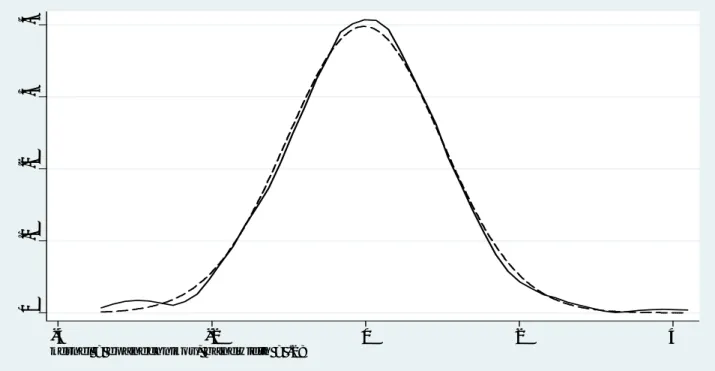
5shows that the empirical distribution of "_bt coincides almost perfectly with the theoretical distribution.

All these adequacy tests seem to con…rm that "t i:i:d:N (0; 1).

5

Conclusion

In this paper, we have shown that the KPSS test and its extension to panel data, suggested by Hadri and Larsson (2005), has a low power against nonstationarity coming from changes in the unconditional variance. CUSUM-based tests allow to …ll this gap. These tests do not compete with the KPSS-based tests and can be considered as complementary to them. CUSUM-based test for panel data is well adapted to …nite samples because the moments of the statistic test are simulated for the small sample sizes. These complementary tests must be applied as follows: First, apply the KPSS-based test. If the null hypothesis is rejected, then conclude that the data contain a unit root, i.e. there is nonstationarity. If the null hypothesis is not rejected, then there is no unit root but a shift in the variance is possible. Then apply the CUSUM-based test. If the null is not rejected, then there is a complete covariance stationarity. Else, if the null is rejected, then conclude that there is no unit root but the data have variance shift and the process is not covariance stationary. An empirical illustration based on the French …nancial index supports our …ndings.

APPENDIX 1 Proof of Theorem 1

i.Since_{b iT} are i.i.d with mean mT and variance 2T the convergence (j) follows from the Lindeberg-Levy

central limit theorem.

ii. We omit index i in the proof and without loss of generality we assume that the intercept is zero. The residuals are et= "t "; " =PTt=1"t=T: It can be shown thatb T can be written as the ratio of

quadratic form in " = ("1; :::; "T)0; i:e:

b T = T 1

"0_C0_AC"

"0_C"

where C = IT 110T 1; IT is the identity matrix of dimension T and 1 is a T -dimensional vector of ones,

and " s N(0; ); =diag(h21; :::; h2T):Let Q represent an orthogonal matrix (i:e:Q0Q = IT) such that

Q 1=2C 1=2Q = D = diag(d1; :::; dT);

where 1=2 _{= diag(h}

1; :::; hT) and let = Q0 1=2C 1=2Q = ( i;j) then the exact moments of b T (see

Jones (1987)) are given by

E(_{b T}) = mT = T 1 Z +1 0 T X i=1 i;i 1 + 2dit (t; d)dt; (15) E(_b2_T) = T 2 Z +1 0 T X i=1 T X j=1 i;i j;j+ 2 i;j (1 + 2dit)(1 + 2djt) (t; d)dt;

where (t; d) =QT_i=1(1 + 2dit) 1=2: For small T , one can use the numerical methods proposed by Paolella

(2003) to compute the moments. But for large T such methods are time consuming and the asymptotic values of E(_{b T}) and E(_b2_T) will be useful. To prove (jj) and (jjj) we need the following

Lemma. Let _b2T =

PT

t=1e2t=T and etare the residuals from regression: yt = r0+ ht"t; "t ii:d:N (0; 1)

where (ht) is a bounded deterministic sequence such that

1 T T X t=1 h2_{t ! h}2_{2 as T ! 1} (16) then 1 T T X e2_t a:s: ! h 2 2: (17)

Proof. Assume that r0= 0. We have et= ht"t h"; h" =PTt=1ht"t=T hence 1 T T X t=1 e2_t = 1 T T X t=1 (ht"t)2 (h")2 (18)

MT = PTt=1ht"t is a square integrable martingale adapted to the …eld zT = ("1; :::; "T) with the

increasing process hMTi = T X t=1 E((ht"t)2j zt 1) = T X t=1 h2_{t ! 1}

The application of theorem 1.3.15 of Du‡o (2003) leads to MT= < MT >! 0 almost surely, this with

(16) imply that h" = 1 T T X t=1 ht"t a:s:_! 0 (19) Likewise MT = XT t=1h 2

t("2t 1) is a square integrable martingale adapted to z; with increasing process

hMTi = 2

XT t=1

4

t, hence theorem 1.3.15. in Du‡o (2003) implies that

1 hMTi T X t=1 h2 t("2t 1) _!0 almost surely on fhM1i = 1g (20)

where hM1i = limT!1hMTi : Since

T X t=1 h2_t !2 T T X t=1 h4_t; (21)

The assumption (16) implies that there exist an universal constants 0 < K1< K2< 1 such that

K1< 1 T T X t=1 h2_t < K2;

this together with (21) implies that hMTi 2T K12 which implies that fhM1i = 1g = and hence

1 hMTi T X t=1 h2_t("2_t 1) a:s: !0; (22)

Since (ht) is a bounded deterministic sequence, then there exists an universal K > 0 such that h4t K for

all t _{1; hence hM}Ti T K for all T , therefore

1 T T X t=1 h2_t("2_t 1) = hMTi T 1 hMTi T X t=1 h2_t("2_t 1) K 1 hMTi T X t=1 h2_t("2_t 1) ;

using (22), it follows that 1 T T X t=1 h2_t("2_t 1) a:s: !0: (23)

Combining (16) and (18), (19) and (23) we obtain (17).

From lemma we deduce that_{b T} has the same limiting distribution as b _T = 1 T2_h2 2 T X t=1 S_t2; St= t X j=1 ej; (24) and hence lim

T!1mT = limT!1E(b T) and limT!1 2 T = lim

T!1var(b T): (25)

Let Dtthe (2; T ) matrix given by

Dt= 0 B B @ t T t T 1 1 0 0 1 C C A

the ones are repeated t times. Since St= e1Dtu;where e1= ( 1; 1)0; u = (u1; :::; uT)0 ut= ht"t; S2t can be

written as a quadratic form in u ; S2

t = u0D0te1e01Dtu . Consequently (see Magnus (1986))

E(S_t2) = trace(D0_te1e01Dt ), = diag(h21; :::; h2T)

= trace( 1=2D0_te1e01Dt 1=2)

= 1=2D0_te1 2

, where kxk2is the Euclidian norm of the vector x.

Now 1=2_D0 te1 2 = t X j=1 h2_j 1 t T 2 + T X j=t+1 h2_j t T 2 (26) = 0 @ T X j=1 h2_j 1 A t T 2 + t X j=1 h2_j 1 2t T

Hence E(b _T) = 1 T2_h2 2 T X t=1 E(S_t2) = 1 T2_h2 2 8 < : T X t=1 0 @ T X j=1 h2j 1 A t T 2 + t X j=1 h2j 1 2t T 9 = ; = 1 h2₂ 8 < : 0 @1 T T X j=1 h2_j 1 A 1 T3 T X t=1 t2+ 1 T2 T X t=1 t X j=1 h2_j 2 T3 T X t=1 t t X j=1 h2_j 9 = ; The convergence (16) implies (see lemma 2 of Boutahar and Deniau (1996)) that

1 T2 T X t=1 t X j=1 h2_{j !} h 2 2 2 1 T3 T X t=1 t t X j=1 h2_{j !} h 2 2 3 Therefore lim T!1E(b T) = 1 3+ 1 2 2 3 = 1 6 (27)

and (jj) follows from (25) and (27). var 1 T2 T X t=1 S2t ! = 1 T4 ( var T X t=1 S2t ! + 2X s<t cov (Ss; St) ) : (28)

Let t= D0te1e01D0t; and 1=2= diag(h1; :::; hT); we have

var(St) = 2trace ( t t ) = 2trace (D0te1e01D0t D0te1e01D0t ) = 2trace 1=2D0_te1e01D0t 1=2 1=2Dt0e1e01Dt0 1=2 = 2 1=2D_t0e1 4 : By using (26) we get var(St) = 2 2 4 0 @ T X j=1 h2_j 1 A t T 2 + t X j=1 h2_j 1 2t T 3 5 2

By using (i), a straightforward computation leads to 1 T4var T X t=1 St2 ! s h 4 2 15T; (29)

where aT s bT means that aT=bT ! 1 as T ! 1: For s < t cov (S_s; S_t) = 2trace ( s t ) = 2trace (D0_se1e01D0s D0te1e01D0t ) = 2trace 1=2D0se1e01D0s 1=2 1=2Dt0e1e01Dt0 1=2 = 2trace ((xx0)(yy0)) = 2(x0y)2; where x = 1=2_D0 te1; y = 1=2D0se1: Since x0= (h1(1 t=T ); :::; hs(1 t=T ); :::; ht(1 t=T ); ht+1t=T; :::; hTt=T ) and y0= (h1(1 s=T ); :::; hs(1 s=T ); hs+1s=T; :::; hTs=T ) : Therefore cov (S_s; S_t) = 2 8 < : s X j=1 h2_j 1 s T 1 t T t X j=s+1 s T 1 t T + T X j=t+1 h2_j ts T2 9 = ; 2 : By using (i), a straightforward computation leads to

1 T4 X s<t cov (Ss; St) s 2h4₂ T4 T X s=1 T X t=s+1 st T + s 1 (s + t) T (t s) s T (30) s h 4 2 90; since T X s=1 T X t=s+1 (ts)2 s T 6 18; T X s=1 T X t=s+1 ts2 s T 5 15; T X _XT s2 s T 4 12:

From (24), (28), (29) and (30) we deduce that var(b _T) = 1 h4₂ var 1 T2 T X t=1 S_t2 ! s 1 45; from this and (25), (jjj) holds.

Proof of Theorem 2. Let us consider model (6). Under H0, we also have ht= h. Hence, it is easy

to see that under the null hypothesis the OLS estimator of r0 is given by rb0 = _T1 PTt=1yt with the

resid-uals given by e_bt = yt rci0 = (r0+ h"t) _T1 PT_t=1(r0+ h"t) = h"t _T1 PT_t=1h"t. To sum up, under the

null hypothesis we have the following results: a) E(e_bt) = 0, b) var(ebt) = h2(1 _T1) and c) For t 6= t0,

E(e_btect0) = (1 T

T2 )h2. Hence theebt’s are asymptotically uncorrelated with a constant variance h2,i.e. white

noise. So thee_bt’s are asymptotically independent and identically distributed as N (0; h2) since "t are

sup-posed to be "t i:i:d:N (0; 1). So the theorem of Inclan and Tiao (1994) is satis…ed for large T . Hence,

T = max t=1;:::;T q T 2 jDtj is asymptotically distributed as W 0 _{= sup} r (jW (r)j when T ! 1, where W (r)

is a Brownian Bridge(weak convergence). Hence conclusion (i) of the theorem holds. From Billingsley (1968), P r W0_{> a = 2}

1

X

k=1

( 1)k+1_{exp( 2k}2_a2_{) = 1 F (a),i.e., F (a) = 1 2} 1

X

k=1

( 1)k+1_{exp( 2k}2_a2₎

is the theoretical distribution function of W0_{. Hence conclusion (ii) of the theorem also holds. The}

con-clusions (iii) and (iv) of the theorem follow from E(W0_{) =} +R1 0

x@F_@x(x)dx = ln(2)p₂ = and var(W0_{) =}

+_R1

0

(x )2 @F_@x(x)dx = ₂[₆ (log(2))2] = 2.

Proof of the corollary. Let us denote by " =) " the weak convergence. Under H0and Assumption 1, the iT’s are independent across i (Assumption.1) and following Theorem 2 they are asymptotically distributed as

random variables which we note by Xi’s having the same distribution as that of W0= sup

r (jW (r)j with mean

E(W0_{) = and variance var(W}0_{) =} 2_{. For a …xed value of N , if T ! 1 we obtain K = p}1 N N X i=1 iT =) _p1 N N X i=1 Xi

. Now if we allow N ! 1, the Lindeberg-Levy central limit theorem applied to fXig

allows us to have _p1 N N X i=1 Xi

=) N(0; 1). According to the theory of the sequential limit (see Phillips and Moon (1999)), we have K _{=) N(0; 1) when T ! 1 and N ! 1.}

References

[1] Ahamada, I.,Jouini, J. and Boutahar, M. (2004), "Detecting Multiple Breaks in Time Series Covari-ance Structure: A nonparametric Approach Based on the Evolutionary Spectral Density", Applied Economics, 36, pp.1095-1101.

[2] Bai,J. and Perron,P. (2003), "Computation and analysis of multiple structural change models", Journal of Applied Econometrics,18(1), pp.1-22,2003.

[3] Boutahar, M. and Deniau, C. (1996), "Least Squares Estimator for regression Model with some Deter-ministic Time Varying Parameters", Metrika,43, pp. 57-67.

[4] Billingsley, P. (1968), Convergence of probability measures. Wiley, New York.

[5] Davidson, R. and Mackinnon J.G.(1998),"Graphical Methods for Investigating the Size and Power Hypothesis Tests", The Manchester School,66, pp.1-26.

[6] Du‡o, M. (1997). Random Iterative Models, Springer-Verlag Berlin Heidelberg.

[7] Hlouskova, J. and Wagner, M.(2006),"The Performance of Panel Unit Root and Stationarity Tests. Results from a Large Scale Simulation Study", Econometric Reviews, 25(1),pp. 85-116.

[8] Hadri, K.(2000), "Testing for Stationarity in heterogeneous panel data", Econometrics Journal,3, pp.148-161.

[9] Hadri, K. and Larsson, R.(2005), "Testing for Stationarity in heterogeneous panel data where the time dimension is …xed", Econometrics Journal,8, pp.55-69.

[10] Harris, R.D.F. and Tzavalis, E. (1999), "Inference for unit roots in dynamic panels where the time dimension is …xed", Journal of Econometrics,90, pp.1-44.

[11] Inclan, C. and Tiao, C.G. (1994), "Use of cumulative sums of squares for retrospective detection of changes of variance", J. Amer. Statist. Assoc, 89, pp. 913-923

[12] Jones, M.C. (1987), "On momenst of ratios of quadratic forms in normal variables",Statistics & Proba-bility Letters,6, pp.129-136.

[13] Kwiatkowski, D., Phillips, P.C.B., Schmidt, P., Shin,Y.(1992), "Testing the the null hypothesis of stationarity against the alternative of a unit root", Journal of Econometrics,54, pp.94-115.

[14] Magnus, J.R. (1986), "The exact moments of a ratio of quadratic forms in normal variables", Ann. Econom. Statist,4, pp.95–109.

[15] Paolella, M.S. (2003), "Computing moments of ratios of quadratic forms in normal variables", Compu-tational Statistics & Data Analysis,42, pp.313-341.

[16] Phillips, P.C.B and Moon, H.(1999), "Linear regression limit theory and nonstationary panel data", Econometrica,67, pp.1057-1111.

[17] Starica, C. and Granger, C.(2005), "Nonstationarities in Stock Returns", The Review of Economics and Statistics,87(3), pp.503-522.

TABLES.

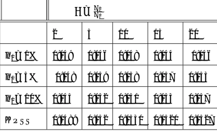
Table 1. The Power of the HL-test and the KPSS-test under the alternative of jumps in the unconditional variance.

= 2 1 2 5 10 15 20 n0= 1% 0:049 0:046 0:048 0:044 0:046 n0= 5% 0:048 0:059 0:058 0:057 0:053 n0= 10% 0:045 0:052 0:051 0:053 0:057 KPSS 0:0489 0:052 0:0530 0:0520 0:0527

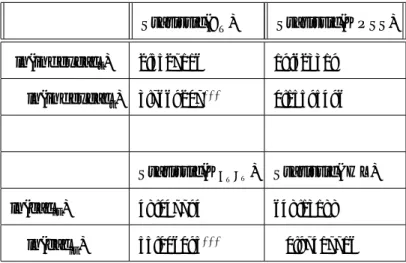
Table 2. Simulated values ofE( iT)and [var( iT)]1=2for each …xed value of T .

========================================================== T 10 15 25 50 100 200 :::::::: 1 — — — — — — — — — — — — — — — — — — — — — — — — — — — — — — — — — — — — — — — — — — — — T 0:6144068 0:6649516 0:71384303 0:7605456 0:7931306 0:81562 ln(2) p 2 ' 0:868 T 0:2273081 0:2399637 0:24905655 0:2535578 0:2579918 0:25907 p 2[6 ln(2)2] ' 0:26 — — — — — — — — — — — — — — — — — — — — — — — — — — — — — — — — — — — — — — — — — — — —

Table 3.The Power of the _T against jumps in the unconditional variance.

1 p1:5 p2 p2:5 p3 2 T = 50 0:030 0:076 0:22 0:363 0:537 0:760 T = 100 0:042 0:193 0:480 0:769 0:90 0:984 T = 200 0:048 0:386 0:860 0:982 0:997 1

Table 4: Nonstationarity in CAC 40

Statistic( _T) Statistic(KPSS) ln(indexcact) 2:5527116 19:623319 ln(indexcac_t) 3:7669207 0:15595496 Statistic(K _T T) Statistic( HL) ln(cacit) 48:047794 648:13188 ln(cac_it) 55:006095 0:97417716

FIGURES.

Figure 1.Performance of the complementary test against abrupt changes in the variance.

0

.2

.4

.6

.8

1

Pow

er

Figure 2. Performance of the HL test against abrupt changes in the variance.

0

.2

.4

.6

.8

1

Pow

er

Figure 3. P-value Discrepancy for the two tests. -.02 -.01 0 .01 P-Va lue D iscrepan cy 0 .2 .4 .6 .8 1 Xi

Complementary test Hadri and Larsson test

Figure 4. bht(horizontal discontinuous line) and returns.

-.1 -.05 0 .05 0 50 100 150 200 250 Time

Figure 5: Kernel density estimate of_b"t(continuous line) and Normal density(discontinuous line)

0

.1

.2

.3

.4

kernel = epanechnikov, bandwidth = .28

Figure.6: Cumulative Periodogram White-Noise Test for_b"t.

0.

00

0.

20

0.

40

0.

60

0.

80

1.

00

C

umu

la

tiv

e

pe

rio

do

gra

m