HAL Id: halshs-00389691
https://halshs.archives-ouvertes.fr/halshs-00389691
Submitted on 29 May 2009
HAL is a multi-disciplinary open access
archive for the deposit and dissemination of
sci-entific research documents, whether they are
pub-lished or not. The documents may come from
teaching and research institutions in France or
L’archive ouverte pluridisciplinaire HAL, est
destinée au dépôt et à la diffusion de documents
scientifiques de niveau recherche, publiés ou non,
émanant des établissements d’enseignement et de
recherche français ou étrangers, des laboratoires
Expectation-Driven Business Cycles
Nicolas Dromel
To cite this version:
Nicolas Dromel. Fiscal Policy, Maintenance Allowances and Expectation-Driven Business Cycles.
2009. �halshs-00389691�
Centre d’Economie de la Sorbonne
Fiscal Policy, Maintenance Allowances and
Expectation-Driven Business Cycles
Nicolas D
ROMELand Expectation-Driven Business Cycles
∗
Nicolas L. Dromel
†May 11, 2009
∗ The author thanks Jean-Michel Grandmont and Patrick Pintus for insightful comments. Special thanks are also due to, without
implicating, Jess Benhabib, Fr´ed´eric Dufourt, Roger Farmer, Cecilia Garc´ıa-Pe˜nalosa, Jang-Ting Guo, Kevin Lansing, Etienne Lehmann, Guy Laroque, Thomas Seegmuller, Alain Venditti, Bertrand Wigniolle, seminar and conference participants at various places for helpful discussions. The usual disclaimer applies.
Abstract
Firms devote significant resources to maintain and repair their existing capital. Within a real business cycle model featuring arguably small aggregate increasing returns, this paper assesses the stabilizing effects of fiscal policies with a maintenance expenditure allowance. In this setup, firms are authorized to deduct their maintenance expenditures from revenues in calculating pre-tax profits, as in many prevailing tax codes. While flat-rate taxation does not prove useful to insulate the economy from self-fulfilling beliefs, a progressive tax can render the equilibrium unique. However, we show that the required progressivity to protect the economy against sunspot-driven fluctuations is increasing in the maintenance-to-GDP ratio. Taking into account the maintenance and repair activity of firms, and the tax deductibility of the related expenditures, would then weaken the expected stabilizing properties of progressive fiscal schedules.
Keywords: Business Cycles; Maintenance and Repair Allowances; Capital Utilization; Progressive Income Taxes;
Local Indeterminacy and Sunspots.
R´esum´e
Les entreprises consacrent un montant significatif de ressources `a la maintenance et `a la r´eparation de leur stock de capital. Dans un mod`ele de cycles d’affaires r´eels pr´esentant de (tr`es) faibles rendements d’´echelle croissants, ce papier ´evalue les effets stabilisateurs de politiques fiscales rendant les d´epenses de maintenance d´eductibles d’impˆot. Dans ce cadre, les entreprises sont autoris´ees `a d´eduire leurs d´epenses de maintenance lors du calcul de leur profit avant impˆot, comme tel est le cas dans nombreux codes fiscaux. Alors que l’imposition proportionnelle ne peut att´enuer l’effet d´estabilisateur d’anticipations auto-r´ealisatrices, il existe un niveau de progressivit´e fiscale pouvant assurer l’unicit´e de l’´equilibre. Toutefois, on montre que ce seuil de progressivit´e stabilisatrice croˆıt avec la part des d´epenses de maintenance dans le PIB. Tenir compte de l’activit´e de maintenance des entreprises et des d´eductibilit´es fiscales associ´ees r´eduirait donc les propri´et´es stabilisatrices attendues de syst`emes fiscaux progressifs.
Mots-cl´es: Cycles d’Affaires; Maintenance et R´eparation du Capital; Utilisation du Capital; D´eductions Fiscales;
Imposition Progressive; Ind´etermination Locale et Tˆaches Solaires.
1
Introduction
An extensive literature has studied the existence of multiple, self-fulfilling rational expectations equilibria in dynamic general equilibrium models. For instance, in a one-sector real business cycle (RBC) model, Benhabib and Farmer [2] and Farmer and Guo [13] have shown that sufficient aggregate increasing returns to scale may give rise to an indeterminate steady state (i.e. a sink) that can be exploited to generate business cycles driven by animal spirits.1 These ”sunspot”
models, where expectations are an independent source of shocks, can motivate stabilization policies designed to mitigate belief-driven cycles. In this line, Guo and Lansing [17] demonstrated that a progressive income tax policy can restore saddle-point stability in the Benhabib-Farmer-Guo model, and thereby stabilize2 the economy against ”self-fulfilling
beliefs”.3 However, this literature assumes that the laissez-faire economy is subject to large and implausibly high
increasing returns to scale (Burnside [7]; Basu and Fernald [1]). As pointed out by Christiano and Harrison ([10] p.20), the desirability of stabilizing the economy against sunspot fluctuations is determined by the relative magnitude of two opposing factors. First, ceteris paribus, a concave utility function implies that a sunspot equilibrium is welfare inferior to a constant, deterministic equilibrium (concavity or risk aversion effect). However, the existence of increasing returns means that by bunching hard work, consumption can be increased on average without raising the average level of employment (bunching effect). As a consequence, when increasing returns are strong enough, the bunching effect may dominate the concavity effect, so that volatile paths may indeed improve welfare, in comparison with stationary allocations. In that situation, one could question the desirability of any stabilization policy.
Recent developments in this research area have relied on increasingly realistic foundations. Many authors have shown that RBC models with multiple sectors of production (Benhabib and Farmer [3]; Perli [25]; Weder [27]); Harrison [19]) or endogenous capital utilization (Wen [29]) may give rise to indeterminacy with smaller increasing returns. Weder [28] introduces a new formulation of the endogenous capital utilization, in which the utilization costs appear in the form of variable maintenance expenses, and shows that indeterminacy can arise at approximately constant returns to scale, challenging the viewpoint that indeterminacy is empirically implausible. In a recent paper, Guo and Lansing [18] explore the effects of introducing maintenance and repair expenditures in Wen’s variable capacity utilization model, and also show that indeterminacy can occur with a mild degree of increasing returns.
1we use the expressions ”animal spirits”, ”sunspots” and ”self-fulfilling beliefs” in a interchangeable way. All of these refer to any
randomness in the economy which is not related to changes in economic fundamentals such as technology, preferences and endowments.
2Here, we adopt the common view that a policy is stabilizing when it leads to saddle-point stability, hence to local determinacy. 3
As a matter of fact, the latest vintages of these models allow to study indeterminacy and sunspots for close-to-constant returns, that is when the ”bunching effect” is (very) weak. One suspects then expectation-driven volatility to unambiguously lead to welfare losses (by the concavity, or risk aversion, effect) that would call for stabilization. This proves useful to re-investigate the stabilizing properties of fiscal progressivity in the close-to-constant returns to scale case, where stabilization is a priori more desirable from a welfare standpoint.
In this paper, we investigate how the stabilizing power of fiscal progressivity, initially pushed forward in this literature by Christiano and Harrison [10] and Guo and Lansing [17], is affected when firms are authorized to deduct their maintenance expenditures from revenues in calculating pre-tax profits (as in many prevailing tax codes4). According
to standard definitions used in the accounting literature, maintenance and repair expenditures are made for the purpose of keeping the stock of fixed assets or productive capacity in good working order during the life originally intended. These expenses involve costs induced to prevent breakdowns (maintenance) and costs to fix of equipment and structures after malfunctioning (repair ). Capital expenditures (investment characterize the purchase of new factories, machines and equipment which ordinarily have a life of more than a year.
In a continuous-time version of the Guo and Lansing [18] maintenance expenditures model, we find that introducing maintenance allowances weakens the expected stabilizing properties of tax progressivity. Although a progressive tax can still render the equilibrium unique, we show that the required degree of progressivity to protect the economy against sunspot-driven fluctuations is increasing in the maintenance-to-GDP ratio. Put differently, the possibility for firms to deduct maintenance and repair expenditures from their pre-tax profits increases the likelihood of local indeterminacy and excess volatility due to animal spirits. Moreover, a flat-tax schedule does not prove to be a useful and effective stabilizer.
Aside from dealing with continuous time and introducing taxation, our paper departs from Guo and Lansing [18] in that we provide clear necessary and sufficient conditions for the stability analysis and do not rely on numerical simulations.
It has been argued and documented (see for instance Mc Grattan and Schmitz [23]), that maintenance expenditures
4As an illustration, in the United States ”it has been held that expenses for small parts of a large machine, made in order to keep the
machine in efficient working condition, were deductible expenses and not capital expenditures even though they may have a life of two or three years” (Commerce Clearing House, Chicago, Standard Federal Tax Reports, 1999, p.22, 182 [9]).
are ”too big to ignore”, strongly procyclical and important potential substitutes for investment. This substitutability feature can be used to provide an intuitive discussion of the basic mechanism driving our result. Let us suppose agents have optimistic expectations about, say, a higher return on capital in the next period. Firms will naturally want to invest more in the form of capital. But, due to the fiscal scheme progressivity, they know they will have to face in that case a higher tax rate. Thus, instead of investing in new physical capital (equipments or structures), firms prefer to substitute maintenance to investment. The consequent reduction in the tax base implies that a higher level of fiscal progressivity will be needed to stabilize the economy against belief-driven cycles.
Our result can be linked to a parallel strand of the literature, investigating the stabilizing properties of non-linear tax schedules in constant-returns-to-scale, segmented asset markets economies (see for instance Lloyd-Braga, Modesto and Seegmuller [22]). In a monetary economy with constant returns to scale, Dromel and Pintus [12] show that tax progressivity reduces, in parameter space, the likelihood of local indeterminacy, sunspots and cycles. However, considering plausibly low levels of tax progressivity does not ensure saddle-point stability and preserves as robust the occurrence of sunspot equilibria and endogenous cycles. Exploiting a different mechanism, our paper gives also support to the view that low levels of tax progressivity may not be able to ensure the determinacy of equilibria.
The remainder of this paper proceeds as follows. The next section presents the model, while section 3 analyzes dynamics and (in)determinacy conditions, showing how fiscal progressivity may lead to saddle-path stability. Some concluding remarks are gathered in section 4.
2
The Economy
This paper introduces fiscal policy, depreciation allowance and maintenance expenditures deductions into a continuous-time version of the Guo and Lansing [18] model. The decentralized economy consists of an infinite-lived representative household supplying labor, and taking real wage as given. The household owns a representative firm, acting in his best interest while making decisions about production, investment, maintenance and capital utilization.
2.1
Firms
There is a continuum of identical competitive firms, with the total normalized to unity, acting so as to maximize a discounted stream of profits. The representative firm i is endowed with k0units of capital and produces an homogeneous
final good yi using the following Cobb-Douglas technology
yi= ¯e(uiki)αn1−αi , 0 < α < 1 (1)
where ki and ni are firm i’s usage of physical capital (equipment and structures) and labor hours, respectively5. The
variable ui ∈ (0, 1) designates the capital utilization rate. Although each firm is competitive, we assume that the
economy as a whole is affected by organizational synergies that cause the output of the ith firm to be higher if all other firms in the economy are producing more. These productive external effects, denoted by ¯e, are outside of the scope of
the market, and cannot be traded. Taken as given by each firm, they are specified as ¯
e = (¯u¯k)αηn¯(1−α)η, η ≥ 0 (2)
where ¯u¯k and ¯n are economy-wide average levels of utilized capital and production labor inputs, respectively. We look
at a symmetric equilibrium, in which all firms would take the same actions such that ui = ¯u = u, ki = ¯k = k and
ni = ¯n = n, for all t. As a result, equation (2) can be substituted into equation (1) to obtain the following aggregate
production technology, that may display increasing returns to scale:
y =£(uk)αn1−α¤1+η (3)
where 1 + η characterizes the degree of aggregate increasing returns. When η = 0, the model boils down to the standard Ramsey formulation with constant returns to scale at both private and social levels.
We assume an endogenous capital depreciation rate, δ ∈ (0, 1), such that
δ = χ u
θ
(m k)φ
, χ > 0, θ > 1, φ ≥ 0 (4) where m represents maintenance and repair expenditures. The ratio m/k denotes the magnitude of the maintenance and repair per unit of capital. When the depreciation elasticity to maintenance (φ) is positive, a rise in maintenance activity will lower capital depreciation. On the other hand, an increase in the capital utilization rate utwill naturally
speed up capital depreciation. If φ = 0, the model resembles the one analyzed in Wen [29], while if θ → ∞, it reduces to an economy with constant utilization like in the standard Benhabib-Farmer-Guo setup.
2.2
Households
The economy is populated by a large number of identical Ramsey households, each endowed with one unit of time, choosing their consumption ctand labor supply nt so as to maximize:
Z ∞ 0 e−ρt ½ log [c] − An 1+γ 1 + γ ¾ dt, (5)
where ρ > 0 is the discount rate, A is a scaling parameter, γ ≥ 0 is the inverse of the intertemporal elasticity of substitution in labor supply. The representative consumer owns the inputs and rents them to firms through competitive markets. We can write down the consolidated budget constraint as:
˙k = (1 − τ)x − c, with x = y − δk − m (6)
where 1 > τ ≥ 0 is the tax rate imposed on the income net of capital depreciation and maintenance expenditures. We assume the capital stock is predetermined k(0) = k0, and both consumption and capital are non-negative k ≥ 0, c ≥ 0.
2.3
Government
The government chooses tax policy τ and balances the public budget at each point in time. Hence, the instantaneous government budget constraint is g = τ x, where g represents government spending on goods and services that are assumed not to contribute to either production or household utility. The aggregate resource constraint of the economy is given by:
c + ˙k + δk + g + m = y
The government is assumed to set τ according to the following tax schedule:
τ = 1 − ν µ ¯ x x ¶ψ , ν ∈ (0, 1); ψ ∈ (0, 1) (7)
where ¯x denotes a base level of income, net of depreciation and maintenance, that is taken as given. Here, ¯x is set to the
steady-state level of that income. The level and slope of the tax schedule are respectively represented by parameters ν and ψ. When ψ > 0, τ rises with the household’s taxable income: households with taxable income greater than ¯x will
have to deal with a higher tax rate than those with an income smaller than ¯x. When ψ = 0, all households face the
taxation. 6 We clearly see at this point that when τ = 0 (i.e. ψ = 0 and ν = 1), even though the model is in continuous
time, it is identical to Guo and Lansing [18].
We assume households take into account the way in which the tax schedule affects their earnings in making decisions about how much to consume, work, invest in new capital, and spend on maintenance of existing capital over their lifetimes. The average tax rate τ , given by (7), is equal to the amount of total taxes paid by each household divided by its taxable income x, while the marginal tax rate τm is defined as the change in taxes paid divided by the change
in taxable income. The expression for τm is
τm=∂(τ x) ∂x = 1 − (1 − ψ)ν µ ¯ x x ¶ψ (8)
In order to prevent government from confiscating all productive resources, we require τ < 1. Besides, we assume
τm< 1 so that households keep an incentive to supply labor and capital services to firms. From (7) and (8), we notice
that τm = τ + νψ(¯x/x)ψ. Therefore, the marginal tax rate will be greater than the average tax rate when ψ > 0
(i.e., the fiscal schedule is ”progressive”). When ψ = 0, average and marginal tax rates coincide at 1 − ν (i.e, the fiscal schedule is ”flat”).
2.4
Intertemporal Equilibria
Households’ decisions follow from maximizing (5) subject to the budget constraint (6), given the initial capital stock
k(0) ≥ 0. Straightforward computations yield the following first-order conditions:
n : Acnγ= (1 − τ m)(1 − α)y n (9) u : α θ y k = δ (10) m : 1 = φδk m (11) k : ˙c c = (1 − τm) α£θ − (1 + φ)¤ θ y k− ρ (12)
where (9) equates the slope of the representative household’s indifference curve (utility trade-off between leisure and consumption) to the after-tax real wage. Equation (12) is the consumption Euler equation. Equation (10) shows that
6However, the present analysis could easily be adapted to the case of weak regressivity (i.e. when ψ < 0), as in Guo and Lansing [17].
For instance, our results still hold if ψ ∈ ((αk− 1)/αk, 1), with 0 < ((αk− 1)/αk) < 1 and αkbeing the elasticity of aggregate output with
the firm utilizes capital such that the marginal benefit of more output equals the marginal cost of faster depreciation. Equation (11) shows that the firm undertakes maintenance activity to the point where one unit of goods devoted to maintenance equals the marginal reduction in the firm’s depreciation expense. Notice that the household’s decisions regarding labor supply and capital investment are governed by the marginal tax rate τm.
We may rewrite the budget constraint, from (6), as:
˙k/k = (1 − τ)x/k − c/k. (13)
Equations (3), (9)-(12) and (13) characterize the dynamics of intertemporal equilibria with perfect foresight, given
k(0).
The transversality condition writes as:
lim
t→+∞e −ρtk
c = 0 (14)
It is easily checked that the transversality constraint is met in the following analysis, as we consider orbits that converge towards an interior steady state. From equation (10), we get δk = (α/θ)y which gives, when plugged into (11),
m = φα θ y
The equilibrium maintenance-to-GDP ratio is constant, and maintenance expenditures perfectly correlated with output. This reminds the procyclicality of maintenance documented by McGrattan and Schmitz [23].
As we want to characterize the reduced-form social technology as a function of k and n, we use equations (7) and (10) to solve7 for u. u = "µ φ θ ¶φµ αy k ¶1+φ#1θ
Then we substitute this optimal rate of capacity utilization into (3) to finally get
y = Bkαknαn
7 Since the parameter χ has no independent influence on the steady state and dynamics around it, we simply set χ = 1/θ. Note that
if we set φ to zero (i.e, capital depreciation is inelastic to maintenance activity), we recover the same optimal capacity utilization as in Wen [29].
where the B, αk and αn write as: B = "µ φ θ ¶φ α(1+φ) # α(1+η) θ−α(1−η)(1+φ) αk = α(1 + η)(θ − 1 − φ) θ − α(1 + η)(1 + φ) (15) αn = (1 − α)(1 + η)θ θ − α(1 + η)(1 + φ) (16)
We restrict our attention to the case where αk< 1 ⇔ 1 > α(1 + η), so that the externality on capital is not strong
enough to generate sustained endogenous growth. We further assume that θ −1−φ > 0 to guarantee αk > 0. Equations
(15) and (16) together imply ∂(αk+αn)/∂φ > 0 whenever η > 0. Hence, a higher degree of aggregate increasing returns
can be achieved through a rise in φ.
2.5
Linearized Dynamics
The dynamics of intertemporal equilibria with perfect foresight, given k(0), are characterized by
˙c c = (1 − τm)α £ θ−(1+φ)¤ θ y k − ρ ˙k k = (1 − τ ) (y−δk−m) k −kc
To facilitate our analysis, we make the following logarithmic transformation of variables: ˆc = log (c), ˆk = log (k) and
ˆ
y = log (y). With this transformation, the equilibrium conditions (9)-(14)can be rewritten as
˙ˆc = αν(1 − ψ)¯xψ £ θ−(1+φ)¤ θ £ θ−α(1+φ)¤ θ −ψ e(1−ψ)ˆy−ˆk− ρ ˙ˆk = ν¯xψ £ θ−α(1+φ)¤ θ 1−ψ e(1−ψ)ˆy−ˆk− ec−ˆˆ k
where ˆc = log (c), ˆk = log (k) and ˆy = log (y).
We can obtain, from the static condition in (12), the following equation: [γ + 1 − (1 − ψ)αn]ˆn = logΓ A + (1 − ψ) log B + (1 − ψ)αkk − ˆc,ˆ (17) where Γ = (1 − α)ν(1 − ψ)¯xψ · θ−α(1+φ) θ ¸−ψ
. This yields, by using equation (17): (1 − ψ)ˆy − ˆk = ξ0+ ξ1ˆk + ξ2ˆc,
where ξ0 = (1 − ψ)Z (18) ξ1 = (1 − ψ)αn+ (γ + 1)[αk(1 − ψ) − 1] γ + 1 − (1 − ψ)αn (19) ξ2 = − αn(1 − ψ) γ + 1 − (1 − ψ)αn (20) where Z = log B + αn γ+1−(1−ψ)αn · log Γ A+ (1 − ψ) log B ¸
. By rewriting equations (12)-(13) in logs and using equations (18)-(20), it is easy to get: ˙ˆc = αν(1 − ψ)(¯x)ψ θ−(1+φ) θ £ θ−α(1+φ)¤ θ −ψ eξ0+ξ1k+ξˆ 2cˆ− ρ, ˙ˆk = ν(¯x)ψ £ θ−α(1+φ)¤ θ 1−ψ eξ0+ξ1k+ξˆ 2cˆ− eˆc−ˆk (21)
It is straightforward to show that, under our assumptions, the differential equations (21) possess a steady state ˆc∗, ˆk∗.
More precisely, ˙ˆc = 0 yields, from the first equation of system (21): exp (ξ0+ ξ1kˆ∗+ ξ2ˆc∗) = ρ αν(1 − ψ)(¯x)ψ θ−(1+φ) θ · θ−α(1+φ) θ ¸−ψ = Ω
On the other hand, ˙ˆk = 0 then yields, from the second equation of system (21): exp (ˆc∗− ˆk∗) = [θ − α(1 + φ)]ρ
α(1 − ψ)[θ − (1 + φ)]= Υ
One can then easily establish that the two latter equations have solutions ˆc∗ and ˆk∗, provided that the scaling
parameter A is appropriately chosen. More precisely, one can set, without loosing generality, ˆk∗ = 0 (that is, k∗ = 1)
by fixing A = Υ−1Ω(1−ψ)αn−(γ+1)αn(1−ψ) Bγ+1αn Γ.
Such a procedure aims at proving the existence of at least one steady state, and at making sure that it ”persists” after any arbitrarily small perturbation of the original two-dimensional map. For a given A, the steady state is unique. On can easily compute the stationary labor supply n∗=
·
(1−α)θ(1−ψ) A[θ−α(1+φ)]
¸ 1
γ+1
, and deduce stationary capital stock k∗=
·
Bα(1−ψ)ν[θ−(1−φ)] ρθ (n∗)αn
¸ 1 1−αk
along with stationary consumption c∗= ρ[θ−α(1+φ)] (1−ψ)α[θ−(1+φ)]] · Bα(1−ψ)ν[θ−(1−φ)] ρθ (n∗)αn ¸ 1 1−αk .
3
Analysis of the Dynamics
Proposition 3.1 (Linearized Dynamics around a Steady State).
Linearized dynamics for deviations ˆc − ˆc∗ and ˆk − ˆk∗ are determined by linear map such that, in steady state:
T = ρ(1+η) © (γ+1)£θ−α(1+φ)¤−(1−α)θª £ θ−(1+φ)α(1+η)¤£γ+1−(1−ψ)αn ¤ D = (γ+1) £ αk(1−ψ)−1 ¤ γ+1−(1−ψ)αn ρ2£θ−α(1+φ)¤ α(1−ψ)£θ−(1+φ)¤ , (22)
3.1
Local Determinacy with Progressive Taxes
Local indeterminacy is defined as follows.
Definition 3.1 (Indeterminacy of the Steady State).
The equilibrium is locally indeterminate if there exists an infinite number of perfect-foresight equilibrium sequences.
While c0 is freely determined by agents in the economy, the variable k is predetermined since k0 is given. Assume
that the stationary state {k∗, c∗} is stable, i.e. all equilibrium trajectories which begin in the neighborhood of {k∗, c∗}
converge back to the steady state. There will be a continuum of equilibrium path {k(t), c(t)}, indexed by c0, since any
path that converges to {k∗, c∗} is necessarily consistent with the transversality condition. Completely stable steady
states generating a continuum of equilibria are called locally indeterminate (i.e., the steady state is a sink).
— Figure 1 about here —
Conversely, if there is a one-dimensional manifold in {k, c} space such that trajectories that begin on this manifold converge to the steady state but all other trajectories diverge then the equilibrium is locally unique in the neighborhood of the steady state. In this case, for every k0 in the neighborhood of k∗ there exists a unique c0 in the neighborhood
of c∗ that generates a trajectory converging to {k∗, c∗}. This c
0 is basically the one that places the economy on the
stable branch of the saddle point {k∗, c∗}.
Since the Trace of the Jacobian measures the sum of the roots and the Determinant measures their product we can use information on the respective signs of the Trace and the Determinant to check the local stability of the stationary state {k∗, c∗}. Indeterminacy prevails as soon as T < 0 < D. The steady-state is saddle-path stable if D < 0, and
unstable (i.e., a source) if T > 0 and D > 0.
— Figure 3 about here —
Let us notice that ν, the parameter characterizing the level of the fiscal schedule, does not appear neither in the Trace, nor in the Determinant (although it affects the steady state, cf. A1). Put differently, ν only affects the level of the steady state, but not the dynamics around it. Hence, when the tax progressivity parameter is set to zero, the flat-rate fiscal structure does not seem to have any effect on the dynamics, in the neighborhood of a stationary state. This result complements some recent conclusions underlining that flat-rate taxation does not promote macroeconomic stability (see e.g., among others, Dromel and Pintus [12], Dromel and Pintus [11]).
Our main task is now to underline the conditions such that the steady state is locally determinate or indeterminate. Direct inspection of equations (22) gives the following Proposition:
Proposition 3.2 (Local Stability of the Steady State).
Assume 0 < αk < 1. Then the following holds: (1 − ψ)αn > γ + 1 is a necessary and sufficient condition for the
occurrence of local indeterminacy. Proof. C.f. Appendix B.
Corollary 3.1 (Local Indeterminacy and Sunspots).
Assume 0 < αk< 1. Then, the following holds:
in the economy without taxes or with linear taxes, (that is, when ψ = 0), the local dynamics of consumption c and capital k given by Eqs. (3) and (12)-(13) around the positive steady state (c∗, k∗) exhibit local indeterminacy (that is
T < 0 < D) if an only if αn> γ + 1.
Corollary 3.2 (Saddle-Path Stability through Progressive Taxation).
and (12)-(13) exhibit saddle-path stability (that is, D < 0) if and only if ψ > ψmin=
(1−α)(1+η)θ−(γ+1)£θ−α(1+η)(1+φ)¤
(1−α)(1+η)θ .
A particular threshold of fiscal progressivity is thus able to immunize the economy from local indeterminacy. However, it is straightforward to show that ψmin is decreasing in θ while increasing in φ (cf. Appendix C). When the tax code
displays some capital depreciation allowance and maintenance/repair deductions (as in the US tax code) the required degree of fiscal progressivity to protect the economy against sunspot-driven fluctuations is increasing in the equilibrium maintenance-to-GDP ratio. Consequently, the possibility for firms to deduct maintenance and repair expenditures from their pre-tax profit tends to weaken the stabilizing power of progressive fiscal schemes established by Guo and Lansing [17] and Guo [15] among others.
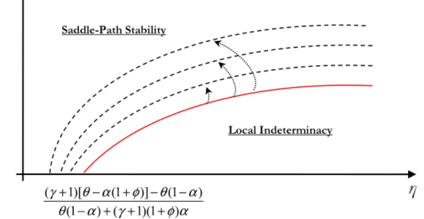
As shown in Fig. 4 and Fig. 5, the geometrical locus depicting the sensitivity of ψmin to η is upward sloping
and concave. An increase in the equilibrium maintenance ratio (achieved though an increase in φ or a decrease in θ) translates this locus upwards (its slope remains exactly the same, regardless of the level of the maintenance-to-GDP ratio) (cf. Appendix D). Hence, for a given level of externalities in the economy, the tax deduction on maintenance and repair expenditures makes local indeterminacy more likely, since a higher level of fiscal progressivity is required to insulate the economy from belief-driven fluctuations.
— Figure 4 and 5 about here —
The recent empirical literature has stressed that maintenance and repair activity is ”too big to ignore” (Mc Grattan and Schmitz [23]): for instance, in Canada, expenditures devoted to maintenance and repair of existing equipment and structures averaged 6.1 percent of GDP from 1961 to 1993. Accordingly, in our theoretical setup, one could possibly expect an arguably high tax progressivity threshold necessary to eliminate indeterminacy.
3.2
Maintenance allowances and tax base reduction
Let us analyze how maintenance activity affects the equilibrium elasticity of social output with respect to labor αn (cf.
maintenance-to-GDP ratio.
The sufficient condition for saddle-path stability in this model is (1 − ψ)αn− 1 < γ
We clearly see that the higher ψ, the lower the left-hand-side, and the lower the likelihood of indeterminacy. Given the fact that the elasticity of output with respect to labor is higher when firms undertake maintenance activity, and a fortiori even more when the maintenance-to-GDP ratio is increased, ψmin (the level of fiscal progressivity needed to
render the equilibrium unique) is also higher.
The procyclicality of maintenance expenditures, assumed in the model, justifies intuitively the excess of volatility added to the economy. On the empirical ground, these procyclical properties have been well-established and documented by Mc Grattan and Schmitz [23]. Using some unique survey data for Canada, these authors find that detrended maintenance and repair expenditures in Canada are strongly procyclical, displaying a correlation coefficient with GDP of 0.89. This Canadian survey also suggests that the activities of maintenance and repair and investment are to some degree close substitutes for each other. For example, during slumps, maintenance and repair expenditures would fall less importantly than investment do. Symmetrically, during booms, maintenance and repair spending would increase less than investment does. The standard deviation of maintenance and repair expenditures is only 60 percent of the investment spending standard deviation (this difference being even sharper in the manufacturing industry). This tends to push forward the idea that during crises, new capital acquisitions would be postponed, and existing equipment/structures would be maintained and repaired to a larger extent. In other words, there would be a good deal of substitutability over the business cycle between maintenance and investment.
This substitutability property can be used to provide an intuitive discussion of the basic mechanism driving our result. Let us suppose agents have optimistic expectations about, say, a higher return on capital in the next period. Firms will naturally want to invest more in the form of capital. But, due to the fiscal scheme progressivity, they know they will have to face in that case a higher tax rate. Thus, instead of investing in new physical capital (equipments or structures), firms will prefer to substitute maintenance to investment. The consequent reduction in the tax base implies that a higher level of fiscal progressivity will be needed to stabilize the economy against belief-driven cycles.
4
Conclusion
Firms devote significant resources to maintain and repair their existing capital. Within a real business cycle model with arguably small aggregate increasing returns, this paper assesses the stabilizing effects of fiscal policies with a mainte-nance expenditure allowance. In this setup, firms are authorized to deduct their maintemainte-nance and repair expenditures from revenues in calculating pre-tax profits, as in many prevailing tax codes. While flat rate taxation does not prove useful to insulate the economy from self-fulfilling beliefs, a progressive tax can render the equilibrium unique. However, we show that the required progressivity to protect the economy against sunspot-driven fluctuations is increasing in the maintenance-to-GDP ratio. Taking into account the maintenance and repair activity of firms, and the tax deductibility of the related expenditures, would then weaken the expected stabilizing properties of progressive fiscal schedules.
Some directions for further research naturally follow. It seems relevant to introduce in this setup, following Guo [15], different progressivity features for labor and capital income, consistent with many OECD countries tax codes. Also, this paper (as many of the contributions in the area) consider fiscal progressivity with a continuously increasing marginal tax rate, which is not a feature shared by most actual tax schedules, as casual observation suggests. Considering linearly progressive taxation instead (as in Dromel and Pintus [11]) could be of interest, in order to get closer to the tax codes with brackets prevailing in most developed economies.
Appendix
A
The Jacobian Matrix
The steady-state Jacobian matrix is derived from: ˙ˆk ˙ˆc = j11 j12 j21 j22 ˆ k − ˆk∗ ˆc − ˆc∗ where j11= ρ£θ − α(1 + φ)¤ α(1 − ψ)£θ − (1 + φ)¤ (ξ1+ 1) j12= ρ£θ − α(1 + φ)¤ α(1 − ψ)£θ − (1 + φ)¤ (ξ2− 1) j21= ξ1.ρ j22= ξ2.ρ
B
Proof of Proposition 3.2
Assume 0 < αk < 1. We can analyze the sign of the steady-state Jacobian’s Trace as follows:
T = >0 z }| { ρ(1 + η)©(γ + 1)£θ − α(1 + φ)¤− (1 − α)θª £ θ − (1 + φ)α(1 + η)¤ | {z } >0 £ γ + 1 − (1 − ψ)αn ¤ (γ + 1)£θ − α(1 + φ)¤− (1 − α)θ can be re-written as γ£θ − α(1 + φ)¤ | {z } >0 + α(θ − 1 − φ) | {z } >0 > 0. We get T < 0, which is a
necessary condition for local indeterminacy, whenever γ + 1 < (1 − ψ)αn. It is easy to check with the steady-state
Jacobian’s determinant that this necessary condition is also sufficient:
D = >0 z }| { (γ + 1) <0 z }| { £ αk(1 − ψ) − 1 ¤ γ + 1 − (1 − ψ)αn >0 z }| { ρ2£θ − α(1 + φ)¤ α(1 − ψ) | {z } >0 £ θ − (1 + φ)¤ | {z } >0
The other necessary condition for indeterminacy, namely D > 0, is obtained whenever γ + 1 < (1 − ψ)αn. Hence,
C
Sensitivity of ψ
minto φ and θ
Since ∂ψmin ∂θ = − α(γ+1)(1+φ) (1−α)θ2 < 0 and ∂2ψ min ∂θ2 = 2α(γ+1)(1+φ)θ(1−α)θ3 > 0, ψmin is convexly decreasing in θ. Moreover, as
∂ψmin ∂φ = α(γ+1) (1−α)θ > 0 and ∂2ψ min
∂φ2 = 0, ψmin is linearly increasing in φ.
D
Sensitivity of ψ
minto η
When the equilibrium maintenance-to-GDP ratio is set to zero (φ = 0 and or θ → ∞), the level of fiscal progressivity ¯
ψmin needed to ensure saddle-path stability is ¯ψmin = (1−α)(1+η)−(γ+1)(1−α)(1+η) . Since ∂ ¯ψ∂ηmin = (1−α)(1+η)γ+1 2 > 0 and ∂ 2ψ¯min
∂2η =
−(1−α)(1+η)2(γ+1) 3 < 0, ¯ψminis concavely increasing. If ¯ψmin= 0, then ηmin|ψmin=0=
γ+α 1−α.
As mentioned earlier in the text, when firms do undertake maintenance activity, and deduct the related expen-ditures from their pre-tax profit, the fiscal progressivity level required to ensure saddle-path stability is ψmin =
(1−α)(1+η)θ−(γ+1)£θ−α(1+η)(1+φ)¤
(1−α)(1+η)θ . Since ∂ψ∂ηmin = (1−α)(1+η)γ+1 2 = ∂ ¯ψ∂ηmin > 0 and ∂ 2ψ min ∂2η = − 2(γ+1) (1−α)(1+η)3 < 0 = ∂ 2ψ¯min ∂2η , we notice that ψmin as a function of (η) exhibits the same slope, whether or not maintenance and repair activity is
effective.
If ψmin= 0, then ηmin|ψmin=0=
(γ+1)[θ−α(1+φ)]−θ(1−α)
(1−α)θ+(γ+1)α(1+φ) . It is easily checked that since
∂η|ψmin=0 ∂θ = (γ+1)2α(1+φ) [(1−α)θ+(γ+1)α(1+φ)]2 > 0 and ∂2η|ψmin=0 ∂θ2 = − (γ+1)2α(1+φ)2(1−α)
[(1−α)θ+(γ+1)α(1+φ)]3 < 0, η |ψmin= 0 is concavely increasing in θ. Moreover, since
∂η|ψmin=0 ∂φ = −[(1−α)θ+(γ+1)α(1+φ)](γ+1)2αθ 2 < 0 and ∂2η| ψmin=0 ∂φ2 = (γ+1)3α2θ2
[(1−α)θ+(γ+1)α(1+φ)]3 > 0, η |ψmin= 0 is convexly decreasing in φ. Given the equilibrium maintenance ratio writes as m
y =φαθ , an increase in this indicator can be achieved though an
increase in φ or a decrease in θ. Consequently, when the equilibrium maintenance-to-GDP ratio rises, η |ψmin= 0 falls.
E
Sensitivity of α
nto φ and θ
Since ∂αn ∂θ = − α(1+η)(1−φ) [θ−α(1−η)(1+φ)]2 < 0 and ∂ 2α n ∂θ2 = 2α(1+η)(1+φ)[θ−α(1−η)(1+φ)] [θ−α(1−η)(1+φ)]4 > 0, αn is convexly decreasing in θ. Moreover, as ∂αn ∂φ = θα(1−α)(1+η)2 [θ−α(1−η)(1+φ)]2 > 0 and ∂ 2α n ∂φ2 = 2θα(1−α)α2(1+η)3[θ−α(1−η)(1+φ)] [θ−α(1−η)(1+φ)]4 > 0, αn is convexly increasing in φ.References
[1] S. Basu, J.G. Fernald, Returns to scale in U.S. production: estimates and implications, J. Pol. Econ. 105 (1997) 249-283. [2] J. Benhabib, R.E.A. Farmer, Indeterminacy and increasing returns, J. Econ. Theory 63 (1994) 19-41.
[3] J. Benhabib, R.E.A. Farmer, Indeterminacy and sector-specific externalities, J. Monet. Econ. 37 (1996) 421-443.
[4] J. Benhabib, R.E.A. Farmer, Indeterminacy and sunspots in macroeconomics, in Handbook of Macroeconomics, 387-448. Eds. J.B. Taylor and M. Woodford. Amsterdam: North Holland.
[5] J. Benhabib, K. Nishimura, Indeterminacy and sunspots with constant returns, J. Econ. Theory 81 (1998) 58-96.
[6] J. Benhabib, Q. Meng, K. Nishimura, Indeterminacy under constant returns to scale in multisector economies, Econometrica 68 (2000) 1541-1548.
[7] C. Burnside, Production function regression, returns to scale, and externalities, J. Monet. Econ. 37 (1996) 177-201.
[8] Canada. Statistics Canada. Various years. Capital and repair expenditures. Annual. Investment and Capital Stock Division, Statistics Canada. Available at http://www.statcan.ca.
[9] Commerce Clearing House (CCH), Standard Federal Tax Reports (7/29/99). Chicago.
[10] L.J. Christiano, S. Harrison, Chaos, sunspots and automatic stabilizers, J. Monet. Econ. 44 (1999) 3-31. [11] N. Dromel, P. Pintus, Linearly progressive income taxes and stabilization, Res. Econ. 61 (2007) 25-29. [12] N. Dromel, P. Pintus, Are progressive income taxes stabilizing?, J. Pub. Econ. Theory 10 (2008) 329-349.
[13] R.E.A. Farmer, J.-T. Guo, Real business cycles and the animal spirits hypothesis, J. Econ. Theory 63 (1994) 42-72.
[14] J. Greenwood, Z. Hercowitz, G.W. Huffman, Investment, capacity utilization, and the real business cycle, Amer. Econ. Rev. 78 (1988) 402-417.
[15] J.-T. Guo, Multiple equilibria and progressive taxation of labor income, Econ. Letters 65 (1999) 97-103.
[16] J.-T. Guo, S. Harrison, Indeterminacy with capital utilization and sector-specific externalities, Econ. Letters 72 (2001) 355-360. [17] J.-T. Guo, K.J. Lansing, Indeterminacy and stabilization policy, J. Econ. Theory 82 (1998) 481-90.
[18] J.-T. Guo, K.J. Lansing, Maintenance Expenditures and Indeterminacy under Increasing Returns to Scale, Int. J. Econ. Theory 3 (2007) 147-158.
[19] S. Harrison, Indeterminacy in a model with sector-specific externalities, J. Econ. Dynam. Control 25 (2001) 747-764. [20] S. Harrison, M. Weder, Tracing externalities as sources of indeterminacy, , J. Econ. Dynam. Control 26 (2002) 851-867. [21] O. Licandro, L.A. Puch, Capital utilization, maintenance costs, and the business cycle, Ann. Econ. Statist. 58 (2000) 143-164. [22] T. Lloyd-Braga, L. Modesto, T. Seegmuller, Tax rate variability and public spending as sources of indeterminacy, J. Pub. Econ. Theory
10 (2008) 399-421.
[23] E.R. McGrattan, J.A. Schmitz Jr., Maintenance and repair: too big to ignore, Fed. Reserve Bank Minneapolis Quart. Rev. 23 (1999) 2-13.
[24] K. Nishimura, K. Shimomura, P. Wang, Production externalities and local dynamics in discrete-time multi-sector growth models with general production technologies, Int. J. Econ. Theory 1 (2005) 299-312.
[25] R. Perli, Indeterminacy, home production, and the business cycle: a calibrated analysis, J. Monet. Econ. 41 (1998) 105-125.
[26] U.S. Department of Commerce. Various years. Expenditures for residential improvements and repairs. Current Construction Reports, C50. Quarterly. Bureau of the Census, U.S. Department of commerce. Available at http:
www.census.gov.
[27] M. Weder, Animal spirits, technology shocks and the business cycle, J. Econ. Dynam. Control 24 (2000) 279-295.
[28] M. Weder, Indeterminacy revisited: variable capital utilization and returns to scale, Finnish Economic Papers, 18 (2005) 49-56. [29] Y. Wen, Capacity utilization under increasing returns to scale, J. Econ. Theory 81 (1998) 7-36.
Figure 1: Local Indeterminacy: the Steady State is a Sink k c c(t) ? k(t) k*
Figure 2: Saddle-Path Stability: the Steady State is Locally Determinate
k(t) c(t) k c k* c*
Figure 3: Jacobian’s Trace-Determinant Diagram: Stability Regimes of Steady State in Continuous Time
D T Sink (locally indeterminate) Source Saddle Saddle
Figure 4: Sensitivity of ψminwith respect to η when the equilibrium maintenance-to-GDP ratio is set to zero Local Indeterminacy Saddle-Path Stability + γ ) 1 ( ) ( α α γ − +
η
ψ
minFigure 5: Sensitivity of ψminwith respect to η when the equilibrium maintenance-to-GDP ratio rises
Local Indeterminacy Saddle-Path Stability + γ