Savings behavior with imperfect capital markets : when hyperbolic discounting leads to discontinuous strategies

HAL Id: halshs-00594060

https://halshs.archives-ouvertes.fr/halshs-00594060

Submitted on 18 May 2011

HAL is a multi-disciplinary open access archive for the deposit and dissemination of sci-entific research documents, whether they are pub-lished or not. The documents may come from

L’archive ouverte pluridisciplinaire HAL, est destinée au dépôt et à la diffusion de documents scientifiques de niveau recherche, publiés ou non, émanant des établissements d’enseignement et de

Savings behavior with imperfect capital markets : when

hyperbolic discounting leads to discontinuous strategies

Bertrand Wigniolle

To cite this version:

Bertrand Wigniolle. Savings behavior with imperfect capital markets : when hyperbolic discounting leads to discontinuous strategies. 2011. �halshs-00594060�

Documents de Travail du

Centre d’Economie de la Sorbonne

Savings behavior with imperfect capital markets : when hyperbolic discounting leads to discontinuous strategies

Bertrand WIGNIOLLE

Savings behavior with imperfect capital

markets: when hyperbolic discounting leads

to discontinuous strategies

Bertrand Wigniolle

April 5, 2011

Paris School of Economics and University of Paris 1 Panthéon-Sorbonne. Address: C.E.S., Maison des Sciences Economiques, 106-112, boulevard de l’hôpital, 75647 Paris Cedex 13, France. Tel: +33 (0)1 44 07 81 98. Email : wignioll@univ-paris1.fr.

Abstract

This paper provides a detailed study of a simple life-cycle consumption model with quasi-hyperbolic discounting and an imperfect …nancial market. It gives a complete characterization of savings behaviors. The joint assump-tions of quasi-hyperbolic discount factors and no-borrowing constraints may lead to non-convexities in selves’ objective functions that may imply dis-continuous equilibrium strategies. Savings function may undergo jumps and non-monotonicities when the income or the interest rate reach a threshold value. These "anomalies" may exist even for reasonable parameters values.

JEL classi…cation: D03, D91

Keywords: quasi-hyperbolic preferences, no-borrowing constraint, discon-tinuous strategies.

1

Introduction

Laibson (1997) analyzes the decisions of a hyperbolic consumer who has ac-cess to imperfect capital markets. He points out that some restrictions on parameters (interest rate and labor income) are necessary to use marginal conditions to characterize the equilibrium strategies. Otherwise, it is possi-ble that selves face a "nonconvex reduced-form choice set" that may generate discontinuous equilibrium strategies. Therefore, he restricts the set of para-meters in order to eliminate this problem.

Some other studies have considered similar frameworks in which the same properties of nonconvexity may occur (e. g. Laibson (1998), Harris and Laib-son (2001)). But they do not focus on the occurrence of these discontinuous strategies. Harris and Laibson (2002) provide the most detailed study of this question. They give an intuition of such strategies. They present the results of numerical simulations, using for labor income a random variable gener-ated by a shift symmetric Beta density. The parameter being the bias for the present of the hyperbolic consumer (with 1), and the relative risk aversion parameter, they show that irregularities in the consumption function tend to disappear when is close to 1 and is high enough. They conclude that discontinuous strategies do not arise when the model is calibrated with empirically sensible parameter values.

The aim of this paper is to challenge Harris and Laibson’s conclusions, in showing that discontinuous equilibrium strategies should not be neglected too soon. Firstly, their conclusions were obtained by numerical simulations with a particular law on labor-income. One aim of this paper is to go beyond these simulation results, by a detailed study of consumption and savings behavior in a simple framework that allows a complete characterization of such strategies.

Secondly, Harris and Laibson’s results are not very surprising. If is close to 1 or if is high, the behavior with hyperbolic discounting is very close to the behavior with exponential discounting. When hyperbolic discounting does not matter, it is not surprising to …nd that discontinuities vanish. On the other hand, if hyperbolic discounting actually modi…es agents’behaviors, it is also associated with discontinuous equilibrium strategies. The value of may also depend on the time duration of the period, and therefore on the frequency of agents’decisions. If the time separating two decisions is long, it can be pertinent to assume that is low. In this case, hyperbolic discounting should have a great e¤ect on behaviors. If the length of the period is short, should be close to 1 and hyperbolic discounting should have a low impact. Thirdly, discontinuous equilibrium strategies can be interesting, as they

provide an example of a behavior that qualitatively di¤ers from the standard model. In the standard model with exponential discount factors, consump-tion behaviors are continuous funcconsump-tions of the di¤erent parameters: interest rates, labor incomes, etc. A consequence of hyperbolic discounting is that a continuous change of one parameter can induce a jump in consumption and savings. Therefore, the two models of consumption and savings lead to results with qualitative di¤erences. They are not observationally equivalent. This paper considers a simple framework to obtain a complete charac-terization of solutions: a three-period quasi-hyperbolic discounting model of life-cycle consumption. At each period the consumer earns some revenue. She/he has access to a …nancial market with a given interest rate on sav-ings. The …nancial market is imperfect in the sense that borrowing is not possible. In periods 1 and 2; selves 1 and 2 strategically choose their amount of savings. The paper studies the Nash equilibrium of this game in which self 1 plays …rst and knows the best response function of self 2: In the lit-erature, this equilibrium is often named the "sophisticated solution". From the assumption of quasi-hyperbolic discounting, the discount factor between period 2 and period 3 is higher for self 1 than for self 2: This discrepancy in preferences may cause a non-concavity of the objective function of self 1; when it is associated with the non-borrowing constraint. For some values of incomes and interest rate, it is possible that self 20s decision to save or not depends on the amount of savings chosen by self 1: At the limit value of self 10_{s savings for which self 2}0_{s savings cancel out, the derivative of self 1}0_s

objective undergoes a positive jump. This jump results from the discrepancy between the preferences of the two selves. In this case, self 10_{s objective}

func-tion may have two local maxima that must be compared to …nd the Nash equilibrium. When some parameter of income or interest rate changes, it is possible that the best strategy of self 1 undergoes a jump from one local maximum to the other one.

These results have important consequences on the properties of the result-ing savresult-ings functions. Some examples are provided for which savresult-ings func-tions can be non-monotonic and may undergo jumps. Initially, the bench-mark calibration of Harris and Laibson (2002) is used. Considering …rst period savings with respect to …rst and second period incomes, it is shown that savings function may undergo a jump upward for some threshold value of incomes. After the jump, there is a signi…cative change in the propensity to save with respect to incomes. Harris and Laibson’s calibration considers an elasticity of substitution equal to 0.5 (a relative risk aversion parameter equal to 2). Increasing the elasticity of substitution allows us to obtain higher jumps in savings function, as the consumer has less taste for consumption

smoothing.

Section 2 presents the model and gives the basic results in the case with-out convexity problems. Section 3 studies the model when the non-borrowing constraint and the quasi-hyperbolic discounting assumption create non-convexity problems. Section 4 gives an overall picture of the results and point out some consequences on savings functions. Section 5 concludes, and Section 6 presents the technical Appendixes.

2

The model

2.1

Basic assumptions

The model is simple, and is restricted to a three-period quasi-hyperbolic discounting model. In period 1, self 1 preferences are given by the utility function: U (c; d; e) = u (c) + u (d) + 2u (e) with u(x) = x 1 1 1 1 (1)

and > 0: c; dand e are respectively the consumption levels in period 1, 2 and 3.

In period 2, self 2’s preferences are given by the utility function: u (d) + u (e)

The budget constraints are:

c + x = A d + y = B + Rx

e = C + Ry

A; B and C are respectively the income amounts earned in period 1, 2 and 3. x and y are …rst and second period savings. R is the factor of interest. and are two positive coe¢ cients not greater than 1. is the usual discount parameter and is the bias for the present.

Capital markets are imperfect: x 0 and y 0: These constraints mean that the agent cannot be indebted1.

The discount factor between period 2 and period 3 is if it is computed by self 1, and if it is computed by self 2. The parameter indicates whether there is a self-control problem ( < 1) or not ( = 1). x is the decision variable of self 1 and y the decision variable of self 2. The sequence of decisions of the agent results from the equilibrium of the game between selves 1 and 2, in which self 1 plays …rst. Therefore, self 2 chooses y; x being taken as given. Self 1 chooses x; taking into account the best response function of self 2.

2.2

Self 2’s behavior

The program of self 2 is: (

max

(y) u (B + Rx y) + u (C + Ry)

s. t. y 0

The solution to this program can be interior (y > 0) or not. De…ning the threshold ~ x 1 R C (R ) B (2)

the best response function of self 2 is:

Y (x) = 8 < : (R ) (B+Rx) C R+(R ) 0 if x x~ if x x~ (3) Y is a non-decreasing function of x:

In the case C B (R ) ; y is always non-negative, even if x = 0: The optimal choice of y is not constrained by the constraint y 0: In the opposite case C > B (R ) ;it is possible that the optimal behavior without

the form: x v and y w: In this case, with the change of variables: x0 _{x + v;}

y0 y + w; A0 A + v; B0 B + w Rv; C C0 Rw; the budget constraints of the

consumer can be written again:

c + x0 = A0 d + y0 = B0+ Rx0

e = C0+ Ry0

the constraint y 0 leads to a negative optimal value for y: In this case the constraint is binding and y = 0: As a consequence, the choice of x by self 1 can determine if self 2 is constrained or not.

2.3

The case

C

B (R

)

This case is simple to study as y is non-negative whatever the choice of x: This is the situation that is considered in general in the literature on savings with hyperbolic discounting.

The optimal behavior of self 1 is obtained in maximizing his objective function, taking into account the best response function of self 2 (3):

( max

(x) u (A x) + u (B + Rx Y (x)) + u (C + RY (x))

s. t. x 0

Replacing Y (x) by the equation (3), this program can be written after some calculations: ( max (x) 1 1 1 (A x) 1 1= +₁11Z B + Rx + C R 1 1= s. t. x 0 (4) with Z = 1 + (R ) 1 [1 + R 1_{( ) ]}1 1= (5)

The solution is:

If R Z A > B + C=R x = R Z A B C R R + R Z x^ (6) If R Z A B + C=R; x = 0:

Using the optimal value of x (either ^xgiven by (6) or 0), it is possible to …nd the equilibrium value of y given by Y (x) (cf. equation (3)).

3

Resolution in the case

C > B (R

)

3.1

The non-concavity of self 1’s objective function

The case C > B (R ) is more interesting as it is possible that the optimal choice of y is positive or 0; depending on the choice of x: The problem of the non-concavity of the objective function of self 1 may occur. To see this, let us consider the objective function of self 1, taking into account the optimal response of self 2. ( max (x) u (A x) + u (B + Rx Y (x)) + 2u (C + RY (x)) s. t. x 0

Taking the derivative with respect to x of this objective function (with x_{6= ~x), we obtain:}

u0(c) + R u0(d) + Y0(x) [ u0(d) + R u0(e)] (7) If the consumer had no problem of self control ( = 1), the expression [ u0(d) + R u0(e)] would correspond to the derivative of self 2’s objective function. This term cancels out ( u0_{(d) + R u}0_{(e) = 0) along the best}

response function of self 2. This is a simple consequence of the envelope the-orem. Therefore, the discontinuity of the derivative Y0 _{in ~xis not a problem}

and the derivative of self 1’s objective function (7) is continuous.

In the case of a quasi-hyperbolic consumer ( < 1), there is a discrep-ancy between the objective functions of self 1 and self 2. From the …rst order condition of self 2, it is obtained that u0_{(d) + R u}0_{(e) = 0; which}

implies u0_{(d) + R u}0_{(e) > 0: Moreover, for x = ~x; the derivative Y}0_{(x) is}

discontinuous: the derivative is 0 to the left of ~x; and is positive to the right. The consequence of this analysis is that the derivative of self 1’s objective function is discontinuous at the point ~x;with a higher value to the right of ~x: It is then possible that self 1’s objective function admits two local maxima. The function is concave on each interval (0; ~x) and (~x; +_{1) and continuous,} but the derivative is discontinuous in ~x:

When the objective function of self 1 has two local maxima, one on the interval (0; ~x) and one on (~x; +_{1) ; it is necessary to compare the values of} the function at these two extrema to …nd its optimal behavior.

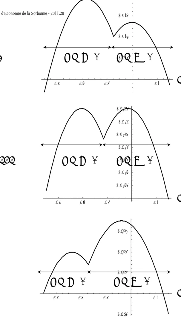
Figure 1 presents a simple numerical simulation with two local maxima for the following values of parameters: = 0:7; = 0:9571; R = 1:0375; = 0:5; A = 12and C = 6: Depending on the value of B; the optimal value of …rst period savings x can imply either y = 0 or y > 0: B = 3:28565 is the threshold value such that the two local maxima are equal.

3.2

Self 1’s objective function

In this part the objective function of self 1 is studied with respect to x; self 1’s decision variable. Two cases are considered: on the interval (~x; +_{1) ; Y (x)} is positive; on the interval (0; ~x) ; Y (x) cancels out. Finally, the solution of the game between selves 1 and 2 is found.

3.2.1 Self 1’s objective function on (~x; +₁₎

First the solution is assumed to be such that y > 0; or (B + Rx) (R ) > C: In this case, the value of x chosen by self 1 is again the solution of program (4). It has been shown that program (4) can lead either to a positive value of x given by (6), or to x = 0: As C > B (R ) ; the solution x = 0 is not compatible with the assumption y > 0; because x = 0 implies y = 0: Therefore, to obtain the case y > 0 as a solution, it is necessary that R Z A > B + C=R; and x is given by (6). Moreover, x being given by (6), to obtain a positive value for y; the study of self 2’s behavior has shown that it is necessary that ^x > ~x. Using (2) and (6), the inequality ^x > ~x leads to:

A +B R >

C

R Z (R ) 1 + R

1_{Z + R} 1_{( ) K (8)}

When C > B (R ) ; as ~x > 0 the inequality ^x > ~x is stronger than ^x > 0: Therefore, if (8) is true, the condition R Z A > B + C=R holds.

To sum up, if (8) is satis…ed, self 1’s objective function has a local maxi-mum ^x_{2 (~x; +1) given by (6), with Y (^x) > 0: If (8) is not satis…ed, self 1’s} objective function is decreasing on (~x; +_{1) ; as the maximum of the objective} function is obtained for a value of x smaller than ~x:

3.2.2 Self 1’s objective function on (0; ~x)

The second type of solution is such that y = 0: In this case, self 1’s program is given by: ( max (x) 1 1 1= (A x) 1 1= + _{1 1=} (B + Rx)1 1= +_{1 1=}2 (C)1 1= s. t. x 0

The solution is: If (R ) A B

x = (R ) A B

If (R ) A < B; x = 0: The objective function is decreasing on the interval (0; ~x); as the maximum is reached for a negative value of x:

In the case (R ) A B; the value of x given by (9) is admissible only if it belongs to (0; ~x) :In the converse case, y should be positive.

Using (9) and (2), the inequality x < ~x leads to A +B

R < C

(R )2 1 + R

1_{( ) L (10)}

To sum up, if (R ) A B and if (10) is satis…ed, self 1’s objective function has a local maximum x 2 (0; ~x) given by (9), with Y (x) = 0: If (10) is not satis…ed, it means that self 1’s objective function is increasing on the interval (0; ~x); as the maximum is obtained for a value of x greater than ~x:

If (R ) A < B; self 1’s objective function is decreasing on the interval (0; ~x):

3.3

The solution of the game between selves 1 and 2

From (8) and (10), it is straightforward to check that K < L as < 1: Therefore, the comparison of the two preceding types of solution leads to the following results.

3.3.1 Solution in the case A + B=R K

If A + B=R K; condition (8) is not satis…ed but (10) holds. From the preceding analysis, it is known that self 1’s objective function is decreasing on the interval (~x; +_{1) ((8) does not hold). On the interval (0; ~x); as (10)} holds, two cases may happen: If (R ) A B; self 1’s objective function reaches a local maximum in x = x > 0 given by (9). If (R ) A < B;self 1’s objective function is decreasing on the interval (0; ~x): From these properties, the result follows:

Proposition 1 If C > B (R ) and A + B=R K; the solution of the game between selves 1 and 2 is:

if (R ) A B; x = x given by (9) and y = 0; if (R ) A < B; x = 0 and y = 0:

These …rst results show that the intertemporal wealth of the consumer during the two …rst periods (A + B=R) plays a crucial role in savings. If this wealth is low and if C is high enough, self 1 has no interest in saving an amount x allowing self 2 to save a positive amount y. Expecting y = 0; the savings choice of self 1 is positive if A is relatively high with respect to B and zero otherwise.

3.3.2 Solution in the case A + B=R L

If A + B=R L; condition (8) holds and condition (10) is not satis…ed: A +B

R

C

(R )2 1 + R

1_{( )}

By assumption, C > B (R ) :These two inequalities imply that (R ) A > B: Therefore it is possible to deduce in this case that:

on the interval (0; ~x); self 1’s objective function is increasing on the interval (0; ~x):

on the interval (~x; +_{1); self 1’s objective function has a maximum ^x:}

Finally, the result is obtained:

Proposition 2 If C > B (R ) and A + B=R L; the solution of the game between selves 1 and 2 is: x = ^x and y = Y (^x):

In this case, the intertemporal wealth of the consumer during the two …rst periods (A + B=R) is high. The optimal behavior of self 1 is to save an amount x high enough to allow self 2 to save a positive amount y.

3.3.3 Solution in the case K < A + B=R < L

When A + B=R < L; the preceding study (section 3.2.2) has shown that two cases may happen, depending on the sign of (R ) A B: Therefore, these two cases are studied separately.

First case: (R ) A B: In this case, previous analysis have shown that self 1’s objective function has two local maxima: on (0; ~x) ; x given by (9) is a local maximum, and Y (x) = 0; on (~x; +_{1) ; ^x given by (6) is another} one, with Y (^x) > 0: To know what is the …nal choice of self 1, it is necessary to compare the value of the objective function at these two points x and ^

x: When x = x and y = 0; the corresponding values for consumption are denoted by c; d and e and the utility level of self 1 is U (c; d; e): When x = ^x and y = Y (^x); the corresponding values for consumption are denoted by ^c;

^

d and ^e and the utility level of self 1 is U (^c; ^d; ^e):

Lemma 1 The values of U (c; d; e) and U (^c; ^d; ^e) are given by

U (c; d; e) = 1 A + B R 1 1 1 + R 1( ) 1 + 1 2_(C)1 1 U (^c; ^d; ^e) = 1 A + B R + C R2 1 1 1 + R 1Z 1 Let us de…ne the function F as:

F ( ) = 1 + C R2 1 1 1 + R 1Z 1 1( ) 1 1 1 + R 1( ) 1 1 2 (C)1 1 F is de…ned in such a way that F (A + B=R) = U (^c; ^d; ^e) U (c; d; e). F is strictly increasing on [K; L] ; with F (K) < 0 and F (L) > 0. Proof. See Appendix 6.1.

This technical lemma allows us to conclude on the optimal behavior of self 1.

Proposition 3 Assume that C > B (R ) ; K < A + B=R < L and (R ) A B: _{There exists M 2 (K; L) such that,}

if K < A + B=R < M; the game between selves 1 and 2 leads to the decisions x = x and y = 0:

if M < A + B=R < L the game between selves 1 and 2 leads to the decisions x = ^x and y = Y (^x)

if A + B=R = M; self 1 is indi¤erent between the two solutions x = x and y = 0; or x = ^x and y = Y (^x):

Following propositions (1) and (2), this proposition shows that for (R ) A B; the line A + B=R = M is the pertinent frontier that separates the two types of savings behaviors: x = ^x and y = Y (^x) or x = x and y = 0.

A consequence of this result is that, if A + B=R is close to M; a small change in one parameter (A; or B or R) can have a dramatic e¤ect on savings behavior: y can jump from 0 to Y (^x); and x can jump from x to ^x: This point will be developed later in Section 4.

Second case: (R ) A < B: In this case, it is not possible to reach the solution x = x; y = 0 associated with (c; d; e): Therefore, the equilibrium of the game between selves 1 and 2 is obtained by the comparison between U (^c; ^d; ^e) and U (A; B; C): The last value of the utility corresponds to the solution x = 0 and y = 0:

Before doing this comparison, it is useful to note that the indirect utility

U (c; d; e) = 1 A + B R 1 1 1 + R 1( ) 1 + 1 2_(C)1 1

can also be interpreted as the utility that self 1 could get in the absence of the constraint x 0 (but with the constraint y 0 which is binding). Consequently, a …rst property is obtained: U (c; d; e) > U (A; B; C): With no constraint on x; it would be optimal to have a negative amount of savings in period 1 as (R ) A < B:

In the case M A + B=R < L, it is easy to conclude. Indeed, it is known that U (^c; ^d; ^e) U (c; d; e)and U (c; d; e) > U (A; B; C): Consequently U (^c; ^d; ^e) > U (A; B; C): The game between selves 1 and 2 leads to the de-cisions x = ^x and y = Y (^x). This result is summarized in the following proposition:

Proposition 4 If C > B (R ) ; (R ) A < B and M A + B=R < L; the solution of the game between selves 1 and 2 is: x = ^x and y = Y (^x):

The case K < A + B=R < M needs a particular study as U (^c; ^d; ^e) < U (c; d; e) and U (c; d; e) > U (A; B; C): Thus, it remains to compare U (^c; ^d; ^e) with U (A; B; C):

The following proposition gives the results:

Proposition 5 Assume that C > B (R ) ; (R ) A < B and K < A + B=R < M: There exists a decreasing function (A) de…ned on [AH; AI] ;

with AH = C (RZ) (R ) 1 + R 1_{( ) ; (A} H) = C (R ) AI = M 1 + R 1_{( )} ; (AI) = M (R ) 1 + R 1_{( )} such that,

if B < (A); U (^c; ^d; ^e) < U (A; B; C) : the game between selves 1 and 2 leads to the decisions x = 0 and y = 0.

if B > (A); U (^c; ^d; ^e) > U (A; B; C) : the game between selves 1 and 2 leads to the decisions x = ^x and y = Y (^x).

if B = (A); U (^c; ^d; ^e) = U (A; B; C) : self 1 is indi¤erent between these two solutions.

Proof. See Appendix 6.2.

Propositions (4) and (5) allow us to conclude when K < A + B=R < L; C > B (R ) and (R ) A < B: When the intertemporal wealth of the consumer during the two …rst periods is high enough (A + B=R M) , the optimal choice for self 1 is x = ^x (and y = Y (^x) for self 2). When A + B=R < M; the choice of self 1 remains x = ^x only if B is high enough with respect to A (B > (A)). In the converse case, self 1 chooses x = 0 and self 2 y = 0.

4

Final results and consequences

4.1

An overall picture of the consumer’s choice

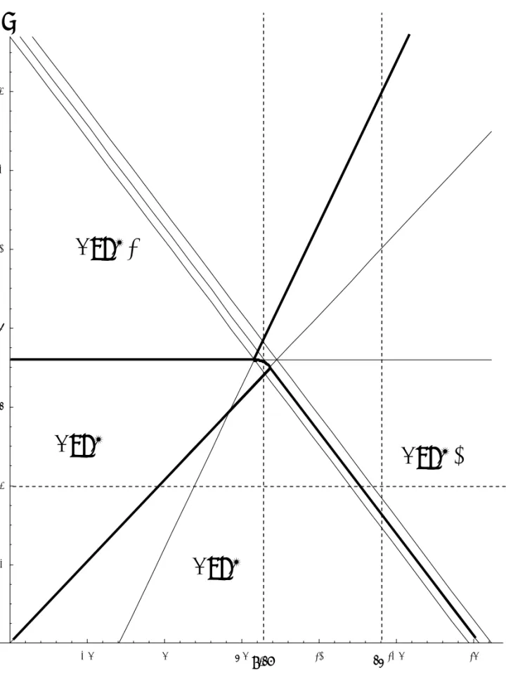
For a given value of the third period income C; it is possible to obtain an overall characterization of the consumer’s savings choices, using the preceding results. Four cases may arise, depending on A and B that allow us to de…ne four sets:

Z1 =f(A; B) s. t. (R ) A > B and A + B=R < Mg

Z2 = (A; B) s. t. (R ) A < B; B < C (R ) ,

Z3 = f(A; B) s. t. A > AH; (RZ) A > B + C=R; B > (A) for A 2 (AH; AI),

A + B=R > M for A > AIg

Z4 = (A; B) s. t. B > C (R ) and (RZ) A > B + C=R

The preceding results give the consumer’s choice in each set2_:

Set 1: x = x given by (9) and y = 0: Set 2: x = 0 and y = 0:

Set 3: x = ^xgiven by (6) and y = Y (^x)given by (3). Set 4: x = 0 and y = Y (0) given by (3).

Figure (2) represents the characterization of the di¤erent zones of the plane (A; B) corresponding to the four sets. The main frontiers are in bold lines. The …gure is obtained for the following values of the parameters: = 0:7; = 0:9571; R = 1:0375; C = 6and = 2:The three …rst parameters are chosen according to the benchmark calibration of Harris and Laibson (2002). The value of is set equal to 2 in order to make more apparent the curve (A): The numerical values have no incidence on the general form of the …gure. In the next part, …gures associated with = 0:5 and = 0:99 will be provided.

4.2

Some consequences of quasi-hyperbolic

discount-ing

The assumption of quasi-hyperbolic discounting can have strong consequences on savings behaviors, when self 1’s objective function is not concave. Di¤er-ent illustrations are provided, with di¤erDi¤er-ent parameters values.

Initially, the benchmark calibration of Harris and Laibson (2002) is used: = 0:7; = 0:9571; R = 1:0375; = 0:5: The value of C is …xed to C = 6: Figure (3) presents the di¤erent zones for these parameter values. The impact of A and B on the amount of savings x is studied. In Figure

2_{To simplify the exposition, the frontiers have not been included in the 4 sets. Indeed,}

for some frontiers corresponding to a discontinuity in the optimal strategy, two di¤er-ent choices are equivaldi¤er-ent for self 1, as it was established in the preceding results (see propositions (3) and (5)).

(4), x is represented as a function of B for two di¤erent values of A : A = 12 and A = 8:163_{. With A = 12; starting from B = 0 and increasing B; the}

incomes of the consumer …rst belong to zone 1, and successively reach zone 3 and 4 (cf. Figure (3)). When B reaches the value such that M = A + B=R; x jumps from x = x to x = ^x > x: The slope of the savings function goes from 0:53 to 0:37.

With A = 8:16; as B increases, the incomes of the consumer belong to zone 1 at the beginning, and successively reach zone 2, 3 and 4 (cf. Figure (3)). In zone 1; x = x and decreases with B till 0: In zone 2; x remains equal to 0: When crossing the frontier (A); xjumps from 0 to a positive value ^x. In zone 3; x = ^xand decreases with B till 0: In zone 4; x remains equal to 0: The e¤ect of A on savings for a given value of B is simulated for B = 4 (cf. Figure (5)). Starting from A = 0 and increasing A; consumer incomes successively cross zones 2, 1 and 3 (cf. Figure (3)). In zone 2, x = 0: In zone 1, x = x and increases with A: When A reaches the value such that M = A + B=R; x jumps from x = x to x = ^x > x: The slope of the savings function goes from 0:44 to 0:61.

The same numerical simulations are done for = 0:99:The overall picture of frontiers is given in Figure (6). The impact of A and B on the amount of savings x is studied. In Figure (7), x is represented as a function of B for two di¤erent values of A : A = 16 and A = 11:13: The values of A are changed with respect to the preceding simulations, in order to obtain the same qualitative features, as the frontiers have moved. Figure (8) shows the evolution of x with respect to A when B is …xed to B = 4: The comparison with the case = 0:5 shows that increasing the elasticity of substitution allows us to obtain more dramatic jumps in savings functions. The same increase in the jumps could be obtained through a decrease of :

In these simple examples, the evolution of savings x with respect to A and B has been considered. It is possible to make the same study with the other parameters. For instance, a jump of savings can also be obtained through a change in the interest factor R:

Our numerical simulations show that savings functions under quasi hy-perbolic discounting present signi…cative di¤erences with respect to the stan-dard case, when discontinuous strategies are taken into account, even for the benchmark parametrization of Harris and Laibson. Firstly, savings functions may undergo upward jumps, resulting from an increase in incomes. Secondly, after these jumps, the slope of savings with respect to income may go up or down.

3_{The value 8:16 corresponds to (A}

These theoretical results may have important consequences for the empir-ical analysis of savings. If agents behave as predicted by the theory, savings functions should be estimated through functional forms able to deal with these jumps and changes in slopes.

5

Conclusion

In this paper, a simple life-cycle consumption model with quasi-hyperbolic discounting and imperfect capital markets has been studied. Using three periods of life for the consumer, it has been possible to reach a complete resolution and a characterization of savings behavior. It has been shown that the savings function may experience discontinuities when consumer in-comes reach some threshold values. These discontinuities may arise even for "reasonable" values of the parameters. They show that quasi-hyperbolic dis-counting can lead to important di¤erences in agents’ behaviors, compared with the standard assumption of exponential discounting.

This paper could be extended in di¤erent directions. Firstly, a technical improvement could be made by introducing more than three periods and more than two decisions. Secondly, discontinuous strategies could be studied in more complex …nancial environment. For example, in an economy with one liquid and one illiquid asset, as in Laibson (1997), discontinuous strategies could exist as a consequence of the non-borrowing constraint on the two assets. Thirdly, discontinuous strategies could exist in other frameworks. For example, Wigniolle (2011) shows that discontinuous strategies can exist in the standard quantity-quality trade-o¤ model of fertility with quasi-hyperbolic discounting. In the problem of the decision of retirement that is analyzed by Diamond and Koszegi (2003), discontinuous strategies could also play a role. In their article, they introduce at some period the retirement decision as a discrete variable. If the time spent working in this period and the retirement time were continuous variables, the existence of discontinuous strategies would become apparent.

6

Appendix

6.1

Proof of lemma (1).

The …rst part of lemma (1) is a straightforward calculation.

The second part is concerned with the study of the function F ( ) = U (^c; ^d; ^e) U (c; d; e) with = A + B=R:

Firstly it is proved that F (K) < 0: The case = K corresponds to the limit case ^x = ~xwhen self 1’s objective function is studied on (~x; +_{1) : From} Section 3.1, it is known that the derivative of self 1’s objective function is discontinuous at the point ~x; with a higher value to the right of ~x: When ^

x = ~x the value of the derivative on the right is 0: Therefore, the value of the derivative on the left is negative. This proves that U (^c; ^d; ^e) < U (c; d; e) or F (K) < 0:

Secondly it is proved that F (L) > 0: The case = L corresponds to the limit case x = ~x when self 1’s objective function is studied on (0; ~x) : From Section 3.1, it is known that the derivative of self 1’s objective function is discontinuous at the point ~x; with a higher value to the right of ~x: When x = ~x the value of the derivative on the left is 0: Therefore, the value of the derivative on the right is positive. This proves that U (^c; ^d; ^e) > U (c; d; e) or F (L) > 0:

Finally, it remains to show that F0_{( ) > 0: The derivative is:}

F0( ) = + C R2 1 1 + R 1Z 1 ( ) 1 1 + R 1( ) 1 The condition F0_{( ) > 0; after some calculations, can be expressed:}

> C 1 + R

1_{( )}

R 1_{[Z ( ) ]} (11)

where it is important to note that Z ( ) > 0: Indeed, from (5), the condition Z > ( ) is equivalent to:

#( ) 1 + (R )

1

[1 + R 1_{( ) ]} 1 > 1

For = 1; #(1) = 1 + R 1 _{> 1: The derivative is}

d ln [#( )] d =

( 1) R 1 2

(1 ) 1 + 1R 1 _{(1 + R} 1₎

For < 1; #( ) is a decreasing function of when < 1 with #(1) > 1: Therefore, #( ) > 1:

For > 1; #( ) is an increasing function of when < 1with #(0) = 1: Therefore, #( ) > 1: Finally, in any case, #( ) > 1 and Z ( ) > 0:

Coming back to condition (11), it remains to prove that this condition holds when K < < M: A su¢ cient condition for that is:

K = C

R Z (R ) 1 + R

1_{Z + R} 1_{( ) > C} 1 + R 1( )

After some calculations, taking into account the expression of Z given by (5), this inequality is equivalent to < 1 which is true by assumption.

6.2

Proof of proposition (5).

The proof is based on the following lemma:

Lemma 2 Assume that C > B (R ) ; (R ) A < B and K < A+B=R < M: Let us consider a given value of C and a given value of = A + B=R with K < < M: A and B may vary in such a way that = A + B=R; with a higher bound Ah_{( ) for A such that A}h_{( ) = = [1 + R} 1_{( ) ] and}

a lower bound Al_{( ) for A such that A}l_{( ) = C= [R (R ) ] : There exists}

an increasing function ( ) that satis…es Al( ) < ( ) < Ah( ) and such that for Al_{( ) < A < ( ); U (^c; ^d; ^e) > U (A; B; C) : the game between selves}

1 and 2 leads to the decisions x = ^x and y = Y (^x).

for ( ) < A < Ah_{( ); U (^c; ^d; ^e) < U (A; B; C) : the game between}

selves 1 and 2 leads to the decisions x = 0 and y = 0.

for A = ( ); self 1 is indi¤erent between these two solutions. The function ( ) is implicitly de…ned by:

u( ) + u [R ( )] + 2u(C) = U (^c; ^d; ^e) Proof:

Let us consider a given value of C and a given value of = A + B=R with K < M: U (^c; ^d; ^e) and U (c; d; e) only depend on and C and they are …xed. For this given value of , it is possible to consider di¤erent values for A and B such that = A + B=R: The highest possible value of A is such that (R ) A = B; and it corresponds to the lowest possible value for B: This gives the values

Ah( ) =

1 + R 1_{( )}

Bl( ) = (R ) 1 + R 1_{( )}

For A = Ah( ) and B = Bl( ); U (c; d; e) = U (A; B; C): Indeed the optimal choice of x without any constraint for x (and y = 0) is such that x = 0: As

U (^c; ^d; ^e) < U (c; d; e) (and < M), it is clear that U (^c; ^d; ^e) < U (A; B; C): The game between selves 1 and 2 leads to the decisions x = 0 and y = 0:

The highest possible value of B is such that C = B (R ) ; and it cor-responds to the lowest value of A: This gives the values

Al( ) = C R (R ) Bh( ) = C

(R )

For B such that C = B (R ) ; ~x = 0:The objective function of self one is concave on (0; +1) : The optimal choice of x again is given by (6). It is positive as

R Z A B C R > 0

Indeed, for A = Al_{( ) and B = B}h_{( ); this inequality becomes:}

> C

R Z (R ) 1 + R

1_{Z + R} 1_{( ) = K}

which is true as > K by assumption. Therefore, in this case, U (^c; ^d; ^e) corresponds to the optimal choice of self 1 and U (^c; ^d; ^e) > U (A; B; C):

Finally, the expression of U (A; B; C) is studied as a function of A and : G(A; ) u(A) + u [R ( A)] + 2u(C)

The derivative @G(A; )=@x is positive as it leads to A 1 R B 1 > 0 _{, (R ) A < B}

G(A; )is an increasing function of A: G is such that G(Al_{( ); )) < U (^c; ^d; ^e)}

and G(Ah_{( ); ) > U (^c; ^d; ^e):Therefore, the existence and uniqueness of ( )}

is proved and

for Al_{( ) < A < ( ); U (^c; ^d; ^e) > U (A; B; C) : the game between}

selves 1 and 2 leads to the decisions x = ^x and y = Y (^x).

for ( ) < A < Ah( ); U (^c; ^d; ^e) < U (A; B; C) : the game between selves 1 and 2 leads to the decisions x = 0 and y = 0.

It remains to prove that ( ) is an increasing function. The function ( ) is implicitly de…ned by: U (A; R ( ) ; C) = U (^c; ^d; ^e); or

1 h ( )1 1 + (R ( ))1 1 + (C)1 1i= 1 + C R2 1 1 1 + R 1Z 1 The derivative 0_{( ) is such that:}

h A 1 R B 1i 0( ) = + C R2 1 1 + R 1Z 1 R B 1 The term A 1 R B 1 is positive as by assumption (R ) A < B: It remains to prove that the right-hand side is positive. To prove that, it is …rst proved that + C R2 1 1 + R 1Z 1 > A 1 this inequality is equivalent to

A 1 + R 1Z > A + B R +

C

R2 (12)

which gives AR 1_{Z > B + C=R: This last inequality is true. Indeed, the}

inequality K < A + B=R leads to A +B R > C R Z (R ) 1 + R 1_{Z + R} 1_{( )} or AR Z > BR Z R + C R + C (R ) 1 + R 1_Z

By assumption, C > B (R ) ; which allows us to write: AR Z > BR Z

R + C

R + B 1 + R

1_Z

that gives AR 1_{Z > B + C=R:Finally, it has been proved that}

+ C R2 1 1 + R 1Z 1 > A 1 As it is assumed that A 1 > R B 1;it implies that

+ C R2 1 1 + R 1Z 1 > R B 1 (13)

Finally, is an increasing function of : Proof of proposition (5).

From the relation A = ( ); it is possible to …nd a relation between A and B given by: B = R [ 1(A) A] (A): It is easy to show that (A) is a decreasing function. Indeed, (A) is implicitly de…ned by U (A; B; C) = U (^c; ^d; ^e); or 1 h (A)1 1 + (B)1 1 + (C)1 1i = 1 A + B R + C R2 1 1 1 + R 1Z 1 (14) The derivative 0_{(A) is such that:}

" R B 1 A + B R + C R2 1 1 + R 1Z 1 # 0_(A) R = A +B R + C R2 1 1 + R 1Z 1 A 1

From the preceding results (cf. (12) and (13)), it is known that

A + B R + C R2 1 1 + R 1Z 1 A 1 > 0 R B 1 A + B R + C R2 1 1 + R 1Z 1 < 0 Therefore 0_{(A) < 0:}

From (14), it is easy to check that (AH) = C (RZ) (R ) 1 + R 1_{( ) =} C (R ) (AI) = M 1 + R 1_{( )} = M (R ) 1 + R 1_{( )}

References

[1] Diamond, Peter & Koszegi, Botond, (2003), "Quasi-hyperbolic discount-ing and retirement," Journal of Public Economics, vol. 87(9-10), pages 1839-1872, September.

[2] Harris, Christopher & Laibson, David, (2001), "Dynamic Choices of Hy-perbolic Consumers," Econometrica, vol. 69(4), pages 935-57, July. [3] Harris, Christopher and David Laibson. (2002), "Hyperbolic

discount-ing and consumption". Mathias Dewatripont, Lars Peter Hansen, and StephenTurnovsky, editors. Advances in Economics and Econometrics: Theory and Applications, Eighth World Congress (1)258-298.

[4] Laibson, David, (1997), "Golden Eggs and Hyperbolic Discounting," The Quarterly Journal of Economics, MIT Press, vol. 112(2), pages 443-77, May.

[5] Laibson, David, 1998, "Life-cycle consumption and hyperbolic discount functions," European Economic Review, Elsevier, vol. 42(3-5), pages 861-871, May.

[6] Wigniolle, Bertrand, (2011), "Fertility in the absence of self-control", working paper n 2011.07, Centre d’Economie de la Sorbonne.

3.4 3.6 3.8 4.2 -0.3228 -0.3227 -0.3226 3.4 3.6 3.8 4.2 -0.3201 -0.3199 -0.3198 -0.3197 3.4 3.6 3.8 4.2 -0.32165 -0.3216 -0.32155 -0.3215 -0.32145 -0.3214 -0.32135

B = 3.28565

B = 3.2

B = 3.4

Figure 1: self 1's objective function for

A = 6,

β

= 0.7,

x

x

x

Y(x) = 0

Y(x) > 0

Y(x) > 0

Y(x) > 0

Y(x) = 0

Y(x) = 0

5 10 15 20 25 30 35 5 10 15 20 25

(RZ)

A=B+C/R

B=A(R

βδ

₎

B=C(R

βδ

₎

M=A+B/R

∆

_(A)

L=A+B/R

K=A+B/R

H

I

A

A

A and B

Zone 2

Zone 1

Zone 4

Zone 3

A

B

2.5 5 7.5 10 12.5 15 2 4 6 8 10 12 14 8.16 12

A

B

Figure 3: the different zones with

σ

= 0.5

Zone 2

Zone 1

Zone 3

Zone 4

E

G

V

A = 8.16

A = 12

Figure 4: savings

x with respect to B

Slope:-0.53 Slope:-0. 37 B = 4,

E

G

V

5 10 15 20 2.5 5 7.5 10 12.5 15 17.5

Figure 6: the different zones with

σ

= 0.99

A

B

11.13 16

E

G

V

A = 11.1288

A = 16

Figure 7: savings

x with respect to B

x B = 4,

E

G

V