HAL Id: halshs-00096821
https://halshs.archives-ouvertes.fr/halshs-00096821
Submitted on 20 Sep 2006
HAL is a multi-disciplinary open access archive for the deposit and dissemination of sci-entific research documents, whether they are pub-lished or not. The documents may come from teaching and research institutions in France or abroad, or from public or private research centers.
L’archive ouverte pluridisciplinaire HAL, est destinée au dépôt et à la diffusion de documents scientifiques de niveau recherche, publiés ou non, émanant des établissements d’enseignement et de recherche français ou étrangers, des laboratoires publics ou privés.
EU Enlargement and the Internal Geography of
Countries
Matthieu Crozet, Pamina Koenig
To cite this version:
Matthieu Crozet, Pamina Koenig. EU Enlargement and the Internal Geography of Countries. Journal of Comparative Economics, Elsevier, 2004, 32 (2), pp.265-279. �halshs-00096821�
EU Enlargement and industrial relocation within the CEECs
∗Matthieu Crozet† Pamina Koenig-Soubeyran ‡
∗We wish to thank Constantin Zaman and Mathilde Maurel for providing data
†TEAM, University of Paris I and CNRS, 106-112 Bd de l’hˆopital 75647 PARIS CEDEX 13, France.
Email: crozet@univ-paris1.fr
‡CREST and TEAM, University of Paris I and CNRS, timbre J360, 15 blvd Gabriel P´eri, 92245 Malakoff
This paper focuses on the relation between trade openness and the location of economic activity in a country. The problematic lies in the context of the EU enlargement process and of its impact on the location of economic activity inside each of the accessing countries. We develop a new economic geography model based on the original Krugman (1991) model, and show that trade liberalization will foster agglomeration of economic activity in the location that has the lowest-cost access to foreign markets. Our results thus differ from Krugman and Livas’s (1996) conclusions. We expect the CEECs’ economies to shift economic activity towards EU markets. We provide empirical evidence of this result focusing on the post-1991 Romanian urban system.
Keywords: economic integration, urban concentration, agglomeration, CEECs
Ce papier se donne pour objectif d’analyser les cons´equences du processus d’´elargissement de l’Union Europ´eenne sur la localisation des activit´es au sein des pays d’Europe Centrale et Orientale . Nous d´eveloppons pour cela un mod`ele d’´economie g´eographique, dans la lign´ee des travaux de Krugman (1991) et Krugman et Livas (1996). Pourtant les conclusions th´eoriques que nous mettons en ´evidence s’opposent clairement celles obtenues par Krugman et Livas (1996). On montre en effet que l’ouverture au commerce peut engendrer un renforcement des dynamiques d’agglomration au sein des pays participant l’´echange. Plus encore, l’ouverture devrait, dans certains cas, favoriser davantage les zones urbaines offrant le meilleur acc`es aux march´es ´etrangers. Dans la derni`ere section de l’article, une analyse empirique centr´ee sur les dynamiques des r´egions roumaines depuis 1991 vient soutenir ces conclusions.
Mots Cl´es : int´egration ´economique, concentration urbaine, agglom´eration, PECO
EU Enlargement and industrial relocation within the CEECs
1
Introduction
The perspective of the enlargement of the European Union (EU) to the Central and Eastern European Countries (CEECs) raises main concern with respect to an eventual reallocation of factors within the accessing countries: the CEECs are about to integrate a new economic struc-ture and are, since the dismantling of the Council for Mutual Economic Assistance (Comecon), significantly overthrown in terms of their trade and production patterns. Therefore, the pre-accession period and the first years after enlargement will be particularly important in observing how the CEECs’ economies react to this shock.
The theory of the Optimal Currency Areas (OCA), enunciated by Mundell (1961), defines an optimal currency area as a set of regions or countries for which the benefits of the monetary union are larger than the costs. The endogeneity argument highlights that commercially integrated countries will endogenously develop conditions to form an optimal currency area: increased trade and diversified economies will favor less asymmetric shocks and thus reduce the costs of having a fixed exchange rate.
Spatial economy and new economic geography literature (Krugman, 1991; Krugman and Venables, 1995; Fujita, Krugman and Venables, 1999) constitute adequate instruments to tackle the issue of the EU enlargement’s impact on production and trade patterns within the CEECs. New economic geography models focus on explaining the emergence of endogenous asymmetrical economic structures. Thus, they represent a very insightful way of analyzing the reaction of the CEECs’ economies to the reorientation of their trade patterns in terms of relocation of industries.
In a national framework, Krugman (1991) and Puga (1998) analyze the geographical distri-bution of economic activity between two regions following an interregional reduction in transport costs; the former model explains specifically how a change in interregional transport costs can lead to the agglomeration of economic activity in one of the two cities, and the latter shows the same phenomenon in a setting incorporating rural-urban migration. Furthermore, and this will be our focus in this paper, the economic geography of a country can also be analyzed in an international framework, as show Krugman and Livas (1996)1
: they study the impact of trade liberalization on the spatial distribution of activity inside a country, and conclude that a country opening to trade will automatically go through a geographical dispersion of its economic activity.
In this paper, we argue that Krugman and Livas’s result does not apply to all situations: by choosing a more general framework, we obtain a less extreme result which states that trade
1
liberalization will foster agglomeration of economic activity in the location that has the lowest-cost access to foreign markets. According to our theoretical results, the more the domestic country opens its economy to the foreign country, the more the domestic industry will be likely to locate in regions that facilitate international trade. Thus, when applied to the European integration process, observing such movements of industry in each of the CEECs would suggest optimistic conclusions about the endogenous course towards an optimal currency area. On the contrary, not observing this reallocation of factors could indicate that the country is withdrawing to itself. In this case it may be that the integration process does not stimulate the country to a closer participation in forming an optimum currency area.
We propose an empirical application based on the Romanian case. We estimate a simple relation connecting the increase in urban population and a measure of access to markets. This allows to assess whether movements of factors towards the western border take place inside the country since the beginning of the accession negotiations.
In section (2) we expose the theoretical model. We present the basic mechanisms underlying endogenous relocation of activity in a two countries framework, when the two domestic regions have the same access to the foreign country. Then, section (3) presents the outcomes of the model when one of the domestic regions has a better access to international markets. Section (4) contains the empirical application, and section (5) concludes.
2
The model
The model we develop in this paper is a simple extension of Krugman’s (1991) model to a two countries framework. At the beginning of our story, the domestic country has no commercial relations with other countries. We are interested in the spatial distribution of economic activity inside the domestic country. In autarky, the situation is the one described by the Krugman (1991) original model: the country develops an economic geography which depends on its in-ternal market’s characteristics: total agglomeration of the manufacturing sector in one of the domestic regions is possible if interregional transport costs are not too high.
When the domestic country opens up to trade with the foreign country, the forces driving the geographic distribution of the increasing returns to scale (IRS) sector change: on the demand side, there is now a new location to supply, containing a consequent amount of consumers (foreign manufacturing and service workers). On the supply side, the foreign firms can now supply the domestic market, enhancing competition for the domestic firms.
We will show different aspects of the impact of trade liberalization on the internal geography of the domestic country: first, we will see that considering a large foreign country around the typical two-regions economic geography model greatly affects the outcome of the model, even if neither the firms nor the consumers are internationally mobile. We will observe that, the larger
the foreign country, the more the domestic industrial sector will be agglomerated in one of the regions. Second, we will show that trade liberalization greatly impacts on the internal geography of the country opening to trade, but not in the way Krugman and Livas (1996)2
conclude. Indeed, our results imply that trade liberalization fosters urban concentration. Finally, we will look at how our results are affected by considering two domestic regions which are not located at the same distance from the foreign market.
2.1 General framework
Consider two countries: a domestic country, containing two regions, labeled 1 and 2, and a foreign country, labeled 0. There are two sectors: one is a monopolistically competitive manu-facturing sector M , which produces a differentiated good and stands for all increasing to scale production activities in the economy. The other is the constant return to scale (CRS), perfectly competitive sector Z, which produces a homogenous good. We can assimilate it to the service industries. The two sectors use specific factors. The manufacturing good is traded between the three regions 0, 1 and 2, while the services good is only traded within the domestic country.
Regional supplies of Z labor are fixed: the three regions contain respectively LZ1, LZ2 and
LZ0workers in the service industries, which are immobile both interregionally and
internation-ally. Concerning the manufacturing sector, only the total amount of M labor is fixed: the foreign country is endowed with L0 industrial workers, which are immobile. The domestic country has
L manufacturing workers, distributed among regions: L = L1+ L2. The interregional domestic
distribution of industrial workers is endogenous: manufacturing workers are mobile and migrate between the two regions 1 and 2, according to the interregional real wage difference.
The spatial framework of the model is introduced through the use of a transport cost variable, representing distance between cities but also, in a broader sense, barriers to trade. We use an ”iceberg”-type transport cost variable, which means that the transport cost is included in the quantity of good shipped. When q units are shipped, each priced p, only a proportion q/τ actually arrives at destination. Therefore, in order for q units to arrive, qτ units have to be shipped, increasing the price of the q units received to qpτ . Trade in the industrial good bears transport costs, which differ across regions: τ is the internal transport cost, which applies to interregional domestic trade, and ρ1and ρ2are respectively the external transport costs applying
to each domestic region’s trade with the foreign country. Trade in the service good only occurs between the two domestic regions and we will assume it is costless, therefore its price equalizes interregionally: pZ1= pZ2. More, it is produced under perfect competition, so the price of the
good equals its marginal cost: pZ1 = βZwZ1 and pZ2 = βZwZ2. As a result both wages are
equalized: wZ1= wZ2= wZ.
2
Consumers and Price indexes
Every consumer has the same Cobb-Douglas utility function:
U = MµZ1−µ (1)
M is a composite index of the consumption of the manufactured good, Z is the consumption of services. A share µ of expenditures goes to manufactured goods, and 1 − µ to the services. The composite index M is the following CES function:
M = " n X i=1 c σ−1 σ i # σ σ−1 (2)
where ci represents the consumption of a variety i of the manufactured good, and σ is the
elasticity of substitution between two varieties. Given income Ys, each consumer maximizes
his utility under the budget constraint Ys = pZZs+Pni=1cipis. We get the following demand
function, representing demand emanating from a consumer of region s, addressed to a producer i located in region r: ci,rs = p −σ irs PR r=0Pn r i=1(pirs) 1−σµYs, r = 0, 1, 2. (3)
Equation (3) contains the spatial framework: there are R regions (R = 0, 1, 2), each of them producing nr varieties of the manufacturing good. The price of each variety i produced in r and
sold in s contains the mill price and the transport cost: pirs = prTrs. We use Trs as a general
expression which represents either τ , ρ1 or ρ2. Using (2) and (3), we are thus able to derive the
following industrial price index for each region s:
Gs= " R X r=1 nr X i=1 (pirTrs) 1−σ # 1 1−σ (4) Producers
Manufactured goods are produced in a monopolistically competitive industry, following the Dixit and Stiglitz (1977) framework. Each producer has the same production function, expressed in terms of manufacturing labor. The total cost contains a fixed cost α and a marginal cost β per additional unit produced:
li = α + βqi (5)
where li is the amount of labor used by each firm and qi represents its production. Each
constant mark-up equations: pi,r= µ σ σ − 1 ¶ wrβ (6)
where wr is the manufacturing wage in region r. The equilibrium output of a firm producing
variety i in region r is derived from the free entry condition: q∗i,r= α(σ − 1)
β (7)
and the equilibrium on the labor market allows us to obtain the equilibrium number of firms in each region:
nr =
Lr
ασ (8)
where Lr is the total number of manufacturing workers in region r.
Wage equations
Finally, using (3), (6), (7), (8) and the equilibrium on the goods market, we derive the manu-facturing wage equation for each region r:
wr= β µ σ − 1 σ ¶ µβ α(σ − 1) R X j=1 YjGσ−1j T 1−σ jr 1/σ (9)
Equation (9) is a typical wage equation in new economic geography models (see Fujita, Krugman and Venables, 1999), containing each region’s income (Yj), weighted by the accessibility of the
region’s demand, the transport costs (Tjr1−σ) and by an index of concentration (Gσ−1j ).
Industrial workers migrate between the two domestic regions, according to the real wage differential. The real industrial wage equation is composed of the nominal wage deflated by the price index:
ωr= wr
Gµr (10)
We now have the principal equations defining the short-run equilibrium of the model at a point in time. For a given allocation of industrial labor between the two domestic regions, and for known parameter values α, β, σ and µ, we obtain instantaneous equilibrium wages and price indexes (w1, w2, G0, G1, G2). If real wages differ across domestic regions, then migration will
make the allocation of industrial labor change over time in order to balance the differential. All workers react in the same way to a real wage difference, therefore interregional movements of workers occur at one go.
The evolution of the spatial distribution of manufacturing towards a more or less asymmetric configuration depends on the interaction of two types of effects: competition effects and demand and cost linkage effects. On the one side, competition effects originate in the high competition on the goods and factors markets that arise when the economy is agglomerated, thus giving an incentive to firms to move to the domestic peripheral market in order to benefit from lower competition on that market. On the other side, the cost and demand linkage effects encourage firms and workers to locate near each other: a large number of workers brings a larger local expenditure, enabling firms to pay higher nominal wages, and making the location more attrac-tive for other workers and firms. A larger number of firms also implies more locally produced varieties, a lower price index, and thus more consumers/workers.
Thus, when competition effects dominate demand and cost linkage effects, the industrial sector will be equally distributed between the two regions. When demand and cost linkage effects dominate competition effects, agglomeration will take place. Both domestic factors (internal transport cost, ...) and international factors (external transport costs, foreign country’s size) can influence the relative importance of competition effects or linkage effects. In this paper we are interested in the evolution of these two effects, and thus, of the spatial distribution of the domestic manufacturing sector when there is a foreign country in the picture. The next section shows how the presence of a foreign country, thus additional demand but also additional competition forces, impacts on the economic geography of the domestic country.
2.2 Increasing the foreign country’s size
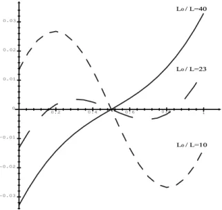
Introducing a foreign country in a Krugman (1991)-type economic geography model brings important changes in the forces involved in determining the final outcome. Figure (1) shows the real wage difference curve ω1− ω2 as a function of the share of manufacturing workers in
region 13
. The curves are drawn for the same parameter values (interregional transport cost τ = 2, both domestic cities having the same external transport cost ρ1 = ρ2 = 3) but for three
different sizes of the foreign country.
The real wage difference curve allows to see the impact of the relocation of one industrial worker from one domestic region to the other on the real wage of the destination region. We first note that, if the symmetric distribution of manufacturing workers is an equilibrium (ω1 = ω2), it
is not always a stable equilibrium: starting at λ = 0.5 and increasing the share of manufacturing workers in region 1 can augment region 1 real wage or decrease it. The evolution of the region 1 real wage and thus, the final equilibrium configuration, will depend on the two types of effects we introduced in section (2.1): competition effect and demand and cost linkage effects. Let’s analyze figure (1) starting with the situation close to the autarky case, in which the domestic country has a reduced access to a relatively small foreign country. The dotted curve represents
3
Figure 1: Real wage difference for three different foreign country sizes -0.03 -0.02 -0.01 0 0.01 0.02 0.03 0.2 0.4 0.6 0.8 1 ✂✁☎✄✆✞✝✠✟☛✡ ✞✁☞✄✌✞✝✎✍✑✏ ✞✁☞✄✌✞✝✎✒✓✡
the evolution of the interregional wage differential when the size of the foreign country relative to that of the domestic country is L0
L = 10. We observe that the wage differential is positive if λ
is less than 1/2, and negative if it is higher than 1/2: thus, the point where the wages are equal is a stable equilibrium. The dashed curve is drawn for an intermediate size of the foreign country: the latter is 23 times larger than the domestic country. We see that the symmetric distribution of industrial workers is still an equilibrium, but that there are now four new equilibria, two of them being polarized and stable, and the two others being unstable. Finally, the dark curve shows the evolution of the interregional real wage difference when the domestic country is surrounded by a huge foreign country of 40 times its size. Whatever value takes λ, the migration of one additional worker from region 2 to region 1 will always augment the real wage in the destination region, which means that the only stable equilibrium is the configuration where manufacturing activity is agglomerated in one of the two regions.
What mechanisms explain the different reactions of the real wage difference to an increase of the industrial labor force in one region? From figure (1) we understand that the size of the foreign country has a significant impact on the linkage effects and the competition effects. Indeed, the impact of the increase in L0 can be analyzed through the effects of its two components: foreign
demand effects and foreign competition effects. Both impact on the linkage effects and the competition effects governing domestic agglomeration or dispersion. On the one side, having an access to a large exterior market lowers the incentive for domestic firms to locate near domestic consumers, which represent a smaller share of their sales. Thus the linkage effects are weakened by the increase in L0; the foreign demand lowers the need to agglomerate near
the competition effects within the domestic country, through the foreign competition effect. The competition exerted by foreign firms on the domestic market is large compared to the competition of other domestic firms. Therefore, the increase in L0 lowers the need for domestic
firms to locate far from domestic competitors, and thus lowers the need to disperse economic activity.
In the present case, where both cities have the same access to the foreign market, the foreign demand effect and the foreign competition effect lower both the incentive for domestic firms to locate near domestic consumers and the incentive to locate far from domestic competitors. As figure (1) illustrates, an increase in L0 diminishes both competition effects and linkage effects,
but has more impact on the competition effect. The demand and costs linkage effects end up dominating the competition effects inside the domestic country, leading the industrial sector to be agglomerated in one of the regions.
2.3 Reducing the international transport cost
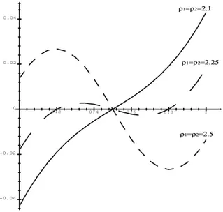
Figure 2: Real wage difference for three different external transport costs
-0.04 -0.02 0 0.02 0.04 0.2 0.4 0.6 0.8 1 ✂✁✄☎✝✆✞✄✠✟✠✡☛ ✂✁✄☎✝✆☞✄✠✟✠✡✌ ✂✁✄☎✍✆✞✄✠✟✠✡✟✝☛
Figure (2) displays the evolution of the interregional real wage difference as a function of the amount of industrial workers located in region 1. The curves are drawn for the same parameter values (τ = 2, L0/L = 10), but for three different values of the external transport cost ρ
4
. As stated before, in this section we consider that neither of the regions has an advantage in exporting to the foreign country: thus, ρ1 and ρ2 are equal and vary together.
4
The dotted curve represents the real wage difference when the external transport cost is ρ1 = ρ2 = 2.5. The only stable equilibrium is the symmetric equilibrium, with one half of the
industrial population located in each region. The dashed curve is drawn for a slightly lower value of the external transport cost. We observe five equilibria, of which three are stable: the symmetric equilibrium and the two asymmetric equilibria. Finally, the dark curve illustrates the interregional real wage difference when the domestic country has an easy access to the foreign market. There is only one stable equilibrium, which is the agglomerated configuration.
This section and the precedent section showed the mechanisms of the model and underlined the main result: trade liberalization fosters agglomeration of the industrial sector in one of the two domestic cities. This result contradicts Krugman and Livas’s (1996) result, which conclude that trade liberalization leads to internal dispersion of economic activity.
Why do we obtain such differing results? The reason lies in the hypotheses leading to the dispersion of the industrial sector. Krugman and Livas’s (1996) model describes the spatial distribution of economic activity inside a domestic country opening to trade, with the typi-cal mechanisms of a new economic geography model based on increasing returns to stypi-cale and transport costs. Yet, their model contains a dispersion force which does not depend on the external transport cost: the congestion costs in a city are commuting costs which only depend on the size of the city, and are not affected by competition pressures arising when the region opens to international trade. The force driving dispersion of activity in Krugman and Livas’s model does not depend on the size of the foreign market, nor on the level of transport costs. Therefore, when opening to trade, the domestic country undergoes a loosening of the incentives for domestic firms to agglomerate near domestic consumers, but no change in the incentive to locate far from domestic competitors. Krugman and Livas thus obtain a dispersed industrial sector as a result of trade liberalization.
3
Pull- and Push-Effects of Trade Liberalization
We will now ask the same question in a lightly different situation: by letting the two external transport costs differ, we suppose that one of the domestic cities has a better access to the foreign markets. We want to know whether this will change the outcome found in the previous section: will the domestic manufacturing sector end up agglomerating in one of the two regions, and if it does, in which city will it agglomerate?
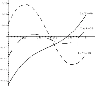
The two following figures illustrate the evolution of the interregional real wage difference as a function of λ, the share of industrial workers in region 1, when a country in which the two cities are not located at equal distance from the foreign market opens to trade. In figure (3), we suppose the following external transport cost structure, where city 2 is located closer to the border than city 1: ρ1= 2.7, ρ2 = 2.3. The three curves are drawn for an internal transport cost
Figure 3: Real wage difference when size of foreign country varies -0.04 -0.03 -0.02 -0.01 0 0.01 0.02 0.03 0.2 0.4 0.6 0.8 1 ✂✁☎✄✆✂✝✟✞✡✠ ✂✁☛✄✆✂✝✌☞✡✍ ✂✁☛✄✎✏✝✒✑✓✠ equal to τ = 25
. In the same way as in the precedent section, we choose in figure (3) to let the size of the foreign country vary. The dotted curve represents the interregional real wage difference when the foreign country’s industrial population is 10 times the domestic industrial population. The domestic country is slightly opened to trade, and the stable equilibrium appears when the industrial activity is dispersed. The dashed and the dark curves represent the situations when the country is confronted to a larger foreign market. At first glance we observe that the impact of trade on the internal economic geography is similar to the one highlighted in section (2): the real wage difference curve progressively changes direction to finally cross the equal wage line with a positive slope, meaning that the stable equilibrium is the situation where the economy is agglomerated in one of the two cities.
Nevertheless, there are two important elements to highlight in the outcomes predicted by figure (3): first of all, the dotted curve, illustrating the stable dispersed equilibrium, crosses the equal wage line at a point which is slightly higher than λ = 0.5, the point where the industrial workforce is equally distributed. This underlines the fact that the situation in which the economic activity is dispersed leaves a population advantage to the remote region. The economy is overall dispersed but there is an asymmetry leading to more than fifty percent of the industrial workers to be located in city 1. This phenomenon emerges because of the greater influence of the foreign competition effect at the beginning of trade liberalization. When external transport costs differ, the foreign competition effect not only lowers the need for domestic firms to locate far from domestic competitors, but also increases their incentive to locate far from
5
foreign competitors, thus pushing domestic firms inside the country towards the border opposite to the foreign market.
The second element to observe in figure (3) concerns the dark curve: the dark curve crosses the equal wage line at a point which is significantly higher than λ = 0.5. This means that although agglomeration is the predicted outcome, it has, in this numerical simulation, more chances to occur in city 2 than in city 1. The agglomeration of the industrial sector will occur in city 2 if city 2 contains 20% or more of the industrial workers. In order for the industrial sector to agglomerate in city 1, which is remote from the border, city 1 would need to be, before trade liberalization, a particularly large industrial center holding more than 80% of the industrial workers. To parallel the push-effect arising from high foreign competition at the beginning of trade liberalization, we highlight the pull-effect arising here from increased trade liberalization. Foreign demand effects dominate foreign competition effects: when external transport costs differ, foreign demand effects not only lowers the need for domestic firms to agglomerate near domestic demand, but also increases their incentive to locate close to foreign demand, thus pulling firms towards the city that has the best access to the foreign market.
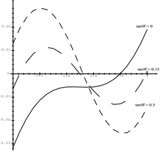
In order to see whether the outcome holds when holding the size of the foreign country constant, we present in figure (4) the situation in which the external transport costs vary. The external transport costs structure is as follows: ρ1 = 2.7 + tariff, ρ2 = 2.3 + tariff. City 2 is
Figure 4: Real wage difference curves when tariff varies
-0.03 -0.02 -0.01 0 0.01 0.02 0.2 0.4 0.6 0.8 1 ✁✄✂☎✆✆✞✝✠✟☛✡☞ ✁✄✂☎✆✆✞✝✠✟☛✡✌✄✍ ✁✄✂☎✆✆✞✝✠✟
thus located closer to the border than city 1. The external transport cost is composed of a fixed element specific to each city, which can be understood as the distance to the border, and of a common element, which is the element we let vary in order to represent trade liberalization.
industrial activity tends to agglomerate in one of the two regions. More, for a strong trade liberalization (when tariff= 0), agglomeration is more likely to concentrate in the region that has the best access to international markets. Thus, the model illustrates that either increasing the foreign country’s size or lowering the external transport costs generate a reallocation of ressources inside the domestic country which has two main characteristics: a push effect can arise, meaning that competition exerted by foreign firms leads to a relocation of economic activity in regions remote from foreign markets as a protection reaction. Nevertheless, the main effect of trade liberalization is likely to be a pull-effect, suggesting that foreign demand attracts domestic firms towards regions that have a good access to foreign markets.
4
Empirical evidence: Urban development patterns in Romania
The empirical literature focusing on the relation between trade and urban structure is mainly concerned with the issue of the impact of an increase in trade on the degree of urban primacy. Ades and Glaeser (1995) study evidence on 85 countries and find a negative relation between trade and urban concentration. They conclude that the data corroborates Krugman and Livas’s (1996) result according to which trade fosters dispersion of industry.
We argue that the relation which to look for in the data is more adequately posed by the model we presented in section (2): trade liberalization is likely to bring several different industry location configurations. These are all explained by the model, which takes into account the fact that cities can be located differently with respect to the main foreign market. Overall, industrial activity will tend to agglomerate close to the foreign markets, but it can happen that because of a specific size advantage, for example, economic activity will locate in the remote city.
Hanson (2001) proposes to estimate such a relation: the analysis aims at verifying whether the theoretical result, according to which trade tends to shift production towards regions with low-cost access to foreign markets, applies to the case of the North-American integration process between Mexico and the USA. Nevertheless, we argue that finding a movement of industries from the inside of the country towards the border close to the foreign market doesn’t necessarily validate Krugman and Livas’s (1996) results. The Mexican case, as well as the Romanian case, on which our empirical work is based, give evidence of a shift of activity towards regions and cities with low-cost access to foreign markets, but do not validate the theory according to which trade liberalization automatically fosters dispersion of economic activity. Henderson (1999), in studying the determinants of urban concentration in a sample of 80 to 100 countries, has a moderate conclusion: the response of urban concentration to increased trade should depend on whether the primate city is already titled towards international markets. According to Henderson’s results, trade will increase urban primacy if the primate city is a port, otherwise it will have the ”economic geography effect, i.e. to help hinterlands by opening up international markets to them” (p. 25).
Our approach in this paper is to not directly link trade to the degree of urban concentration but to the geographical location of cities. The theoretical result arising from our model presented in section (2) suggests that industrial activity will tend to locate in the city that has the best access to foreign markets. We choose to estimate whether such movements of activity can be found in countries opening up to trade such as the CEECs.
The perspective of the enlargement of the EU to the CEECs offers an very interesting frame-work in which to study these issues. First, the CEECs are about to integrate a new economic structure. All the CEECs signed the Europe Agreements, which provide a framework for their gradual integration into the EU and are likely to generate new trade flows between the two areas. Therefore, the current process of integration of the CEECs in the EU represents a ade-quate natural empirical experiment on which to estimate the magnitude of the relocation effects predicted by the traditional new economic geography models. Second, the CEECs undergo significant changes in their trade patterns: Maurel and Cheikbossian (1997) mention that since the dismantling of the COMECON in 1991, a rapid reorientation of the CEECs’ trade has taken place. The intra-COMECON commercial relations fell abruptly and the CEECs have opened their economies towards western countries and primarily to the EU. It seems therefore appropri-ate to study each of these countries in the framework presented by a new economic geography model analyzing the relation between trade liberalization and the location of industry inside a country.
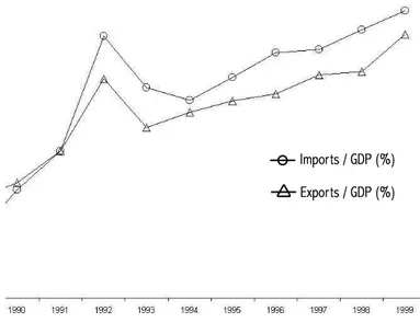
Romania, as all CEECs, undergoes a significant change in its trade patterns. Figure (5) portrays Romanian exports and imports to and from western European countries in percentage of GDP for the period 1988 to 19996
. The figure shows that Romanian imports increased for the whole period, with a peak around 1992 and a decrease in 1993. The weight of western European goods in Romanian consumption thus rose significantly during the time period we study in our sample. In the same way, exports to western Europe augmented consequently in percentage of GDP, highlighting an increased participation of Romania in its commercial relations with the EU and other European countries.
A second reason why Romania is a good candidate for our empirical work is its internal geography. Indeed, Bucharest lies at the opposite of the western border: this specific location of the main city will make any supposed movement of industry and population towards EU markets more visible if industrial activity tends to leave the capital to locate in western regions. Finally, Romania, as far as its economic situation is concerned, doesn’t bear the charac-teristics of the perfect candidate for EU accession. Insufficient progress in adopting a market economy, but also a location remote from EU’s core, are elements which let us expect relatively high adjustment costs in terms of the country’s specialization patterns and production struc-ture. The present work can thus be of some help in understanding the tendance followed by the
6
Figure 5: Romania-Western Europe trade
✁✄✂✆☎✞✝✠✟☛✡✌☞✎✍✑✏✓✒✕✔☛✖✘✗
✙✛✚✜✂✢☎✣✝✠✟☛✡✌☞✎✍✑✏✓✒✕✔☛✖✘✗
Romanian economy during the last ten years. Indeed, if pull-effects dominate push-effects, i.e. if the outcomes display a pattern of urbanization concentrated in regions with a low-cost access to EU markets, it could highlight a positive consequence of the deepening of the integration process between Romania and the EU, giving evidence of the willingness and the readiness of Romanian firms in trading with western European partners. As mentioned before, according to the optimum currency area theory, the costs of EU accession for Romania in terms of production adjustments should be lower the more the country’s economy shows marks of openness to the core.
4.1 Specification and data
In the model we developed in section 2 and 3, in the same way as in new economic geography models, industrial workers migrate towards regions with higher real wage. A region’s real wage is defined, as illustrated by equation (10), as the ratio of the nominal wage on the industrial price index. Therefore, an implication of the model would be to find, within Romania, significant workforce and firms movements towards regions characterized by higher nominal wages -equation (9)- and lower price indexes - -equation (4). Accordingly, we want to estimate a relation assessing whether during the last decade, any significant movement of population towards the western cities, and thus, any increase in the degree of urbanization was to be seen in the regions that have higher nominal wages and a good access to the EU markets: as we will explain in this section, we use a computed market potential variable instead of the industrial price index, because these two variables relate in significant ways.
Urban development
Our measure of the increase of the degree of urbanization is based on annual regional population data, divided among rural and urban population. We calculate regional urban balances, and we express the share of urban population sur of a region r as the ratio of urban population to total population. The annual growth rate of the ratio of urban population is then defined as the difference of the logarithms.
Population data is provided by the Romanian Statistical Office. It consists of regional population data for the years 1991 to 1998, separated in urban and rural population. Romanian regions correspond to the Eurostat classification at the NUTS 3 level, which divide the country in 41 entities, Bucharest and its suburbs being one region.
The geography of growing urban population is the following: regions whose share of urban population increased between 1993 and 1997 are either the regions containing medium size Romanian cities (RO054, Timisoara; RO063, Cluj) or western and southern border regions (RO041, Dolj; RO061, Bihor).
Access to markets
The real wage, according to which industrial workers migrate, contains the nominal wage and the price index. The price index of a region shows high similarity with its market potential, which is a measure of access to markets typically used in new economic geography models. It was first enunciated in a simple form by Harris (1954), as the distance-weighted sum of all other region’s GDPs: M Ptr = N X j=1 GDPtj drj (11)
where drs is the distance between region r and s.
It is thus possible to emphasize the similarity between the price index of a region and that region’s market potential, according to Harris’s definition: both contain the distance weighted-number of firms in each region. The closer region r is from an economic core, the higher is its market potential, and the lower is its industrial price index. Thus, we compute the simple market potential variable for each region from GDP and distance data and use it as a variable explaining the urbanization patterns.
We choose to divide the market potential into three parts, corresponding to three different markets: EU markets, CEECs’ markets (but Romania) and domestic Romanian market. As emphasized earlier, regressing the urbanization patterns on the access to three different markets is likely to highlight the dynamics underlying the reallocation of ressources in Romania. It will allow to see whether Romania is reorienting its production structures towards western or central European markets, or on the contrary if Romania is withdrawing to itself.
GDP data come from the Eurostat Regio database. We use regional data for EU countries and national data for CEECs. Distances are provided by an electronic road atlas.
We regress the urbanization growth rate on the three market potentials and on the following variables: the wages and the unemployment rate, the share of agricultural employment in total regional employment, and two dummies corresponding to port cities and to the capital city.
4.2 Results
Tables (1) and (2) present the estimation results. Both group of estimations are done using fixed effects on the time dimension. This allows to take into account heterogeneity in urbanization patterns arising from particular years. Thus, our coefficients only reflect heterogeneity in the degree of regional urbanization resulting from spatial characteristics.
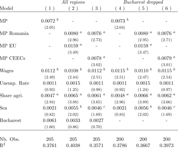
Table 1: Urban Growth in Romania 1993-1997 - OLS Fixed Effects Dependent variable: Annual growth rate of share of urban population
All regions Bucharest dropped
Model ( 1 ) ( 2 ) ( 3 ) ( 4 ) ( 5 ) ( 6 ) MP 0.0072 b - - 0.0073 b - -(2.05) (2.04) MP Romania - 0.0080 a 0.0076 a - 0.0080 a 0.0076 a (2.96) (2.73) (2.95) (2.71) MP EU - 0.0159 a - - 0.0159 a -(3.49) (3.47) MP CEECs - - 0.0078 a - - 0.0079 a (3.02) (3.01) Wages 0.0112 b 0.0108 b 0.0112 b 0.0115 b 0.0110 b 0.0115 b (2.49) (2.44) (2.51) (2.51) (2.47) (2.54) Unemp. Rate 0.0011 0.0015 0.0011 0.0011 0.0015 0.0011 (0.93) (1.25) (0.98) (0.92) (1.24) (0.97) Share agri. 0.0047 a 0.0065 a 0.0061 a 0.0048 a 0.0066 a 0.0062 a (2.94) (3.88) (3.65) (2.96) (3.89) (3.66) Sea 0.0021 0.0055 b 0.0046 c 0.0021 0.0056 b 0.0046 c (0.82) (2.02) (1.69) (0.83) (2.02) (1.69) Bucharest 0.0061 0.0033 0.0027 - - -(1.60) (0.86) (0.70) Nb. Obs. 205 205 205 200 200 200 R2 0.3761 0.4038 0.3571 0.3786 0.3667 0.3973
Table 1 displays estimation results for the 1993-1997 period. The four top rows display the parameter estimates for the principal variable of interest: the access to markets. The first column only contains the total market potential. It is positive and significative, but we note that the coefficient on the market potential variable is higher when the variable is divided among geographical regions: column (2) comprises results concerning the Romanian and the European market potential, and column (3) for the Romanian and the CEECs market potential. In both columns, the coefficients on the market potential are higher and more significative than in column (1). More, there are differences among geographical areas: access to European markets seems to have a stronger influence on Romanian urbanization patterns than access to the domestic market. Concerning the CEECs, the influence is lower than that of European countries, but we observe that it is still slightly higher than the influence of Romanian markets. Thus, trade liberalization seems to give more weight to the proximity to European markets in Romanian workforce location decisions. This is a positive finding with respect to the dynamics possibly reshaping central and eastern European production structures: cities grow faster in regions that have a good access to EU markets, and also, but in a weaker way, to CEECs markets.
The three last columns present estimation results obtained without taking into consideration the Bucharest observation. We note that the results are unchanged: having a low-cost access to European markets still appears to have the strongest influence on Romanian urbanization patterns. Thus, it is interesting to note that the capital city doesn’t behave like a city which has some advantage in foreign trade. More, Bucharest doesn’t seem to be an observation bringing much information to the estimation, as emphasized by the non significative Bucharest dummy variable in the first three columns. This variable is thus dropped in the next three columns.
The share of agricultural employment in total employment represents a dummy variable for a region’s low density, or, alternatively, for low congestion costs. In all columns, the share of agricultural employment is positive and significative. Everything equals, this means that the more a region is agricultural, thus not very dense, the higher will be its urban growth rate. This variable takes into account the fact that it is easier to have a high urban growth rate when there is little urbanization at the beginning.
The Sea variable is a dummy representing regions that are likely to have a good access to foreign markets because they contain or are located near a port city. This variable is rarely significative, highlighting that a maritime location doesn’t constitute an important element in favoring urban development.
Table (2) displays estimation results obtained by dividing the sample into three periods. We still use fixed effects on the time dimension, in order to control for the heterogeneity arising from different years. Our coefficients thus only contain a spatial dimension. Comparing them
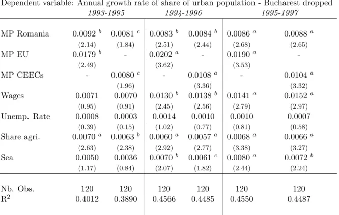
Table 2: Urban Growth in Romania by period - OLS Fixed Effects
Dependent variable: Annual growth rate of share of urban population - Bucharest dropped
1993-1995 1994-1996 1995-1997 MP Romania 0.0092 b 0.0081 c 0.0083 b 0.0084b 0.0086 a 0.0088 a (2.14) (1.84) (2.51) (2.44) (2.68) (2.65) MP EU 0.0179 b - 0.0202a - 0.0190 a -(2.49) (3.62) (3.53) MP CEECs - 0.0080c - 0.0108 a - 0.0104 a (1.96) (3.36) (3.32) Wages 0.0071 0.0070 0.0130 b 0.0138b 0.0141 a 0.0152 a (0.95) (0.91) (2.45) (2.56) (2.79) (2.97) Unemp. Rate 0.0008 0.0003 0.0014 0.0010 0.0010 0.0007 (0.39) (0.15) (1.02) (0.77) (0.81) (0.58) Share agri. 0.0070 a 0.0063 b 0.0060a 0.0057 a 0.0068 a 0.0066 a (2.63) (2.38) (2.92) (2.77) (3.38) (3.27) Sea 0.0050 0.0036 0.0070 b 0.0061c 0.0080 a 0.0072 b (1.17) (0.84) (2.07) (1.82) (2.44) (2.24) Nb. Obs. 120 120 120 120 120 120 R2 0.4012 0.3890 0.4566 0.4485 0.4550 0.4487
t-student in parentheses - a, b and c indicate significance at the 1, 5 and 10 % level
among three different periods allows to assess whether proximity to a particular market has become more influent on regional urbanization over the time period considered.
Observing the first column of each time period shows the evolution of the relative impor-tance of Romanian and European markets in influencing Romanian urbanization patterns. The Romanian market does appear to have some importance, as shown by the positive and signi-ficative coefficients. Proximity to European countries is also positive and signisigni-ficative. We can emphasize that over the three periods, European markets have a higher influence on Romanian urbanization patterns than the domestic Romanian market, even if this relatively higher coef-ficient doesn’t always increase from one period to another. The second column of each time period illustrates the evolution of the coefficients on Romanian and CEECs’ market potential variables. While both markets seem similarly important to Romanian location decisions during the first period, we note that the CEECs take much more weight starting at the second period. Nevertheless, the coefficient of the CEECs market potential never attain the value showed by the European market potential.
The results displayed in table (2) stress interesting features characterizing Romanian ur-banization patterns. First, the more the period is distant from 1991, the more proximity to all markets affects Romanian workforce and firms location decisions. This may express the fact that the Romanian production and location dynamics are slowly becoming independent of
authori-tarian decisions. Second, the influence of foreign markets is always higher than that of domestic markets, and, within foreign markets, European countries are the most influent. This reflects location dynamics increasingly turned towards western markets, which is a positive conclusion for analyses based on the optimum currency area argument.
5
Conclusion
The theoretical contribution of this paper is based on a simple extension of the original Krugman (1991) new economic geography model to a two countries framework. Our theoretical model shows that trade liberalization is likely to lead to the agglomeration of economic activity towards regions that have a good access to foreign markets. Thus, unlike Krugman and Livas’s (1996) conclusions, our results predict a domestic reallocation of ressources that depends on the internal geography of the country opening to trade.
The Romanian process of trade liberalization towards the EU constitute our empirical appli-cation. Estimation results display a positive relation between the degree of regional urbanization and the proximity to western markets, highlighting workforce and production location dynamics bending towards EU markets. While the Romanian case confirms our theoretical prediction, it doesn’t constitute a sufficient experiment to assess the prevalence of our theoretical results. We will need to work on a broader sample in order to emphasize the agglomeration of economic activity towards regions with low-cost access to foreign markets, whatever the initial internal geography may be.
Nevertheless, the Romanian case does bring interesting and positive conclusions with respect to the Optimum Currency Area theory: the country’s internal dynamics appear to be definitely tilted towards European markets, which stresses the visible consequences of the starting inte-gration process. Romania seems likely to develop endogenously the adequate characteristics in order to minimize the costs of fixing its exchange rate.
References
Ades A. and E. Glaeser, 1995, “Trade Circuses: Explaining Urban Giants”, Quarterly Journal of Economics, 110 (1): 195-227.
Alonso Villar O., 2001, “Large Metropolises in the Third World: an Explanation”, Urban Studies, 38 (8): 1359-1371.
Alonso Villar O., 1999, “Spatial Distribution of Production and International Trade: a note”, Regional Science and Urban Economics, 29 (3): 371-380.
Dixit A. and J. Stiglitz, 1977, “Monopolistic Competition and Optimum Product Diver-sity”, American Economic Review, 67 (3): 297-308.
Fujita M., P. Krugman et A. Venables, 1999, The Spatial Economy, Cambridge, MIT Press.
Hanson G., 2001, “US-Mexico Integration and Regional Economies: Evidence from Border-City Pairs”, Journal of Urban Economics, 50 (2): 259-287.
Harris C., 1954, “The Market as a Factor in the Localization of Industry in the United States”, Annals of the Association of American Geographers, 64: 315-348.
Henderson V., 1999, “The Effects of Urban Concentration on Economic Growth”, mimeo, Brown University.
Henderson V., T. Lee and Y.J. Lee, 2001, “Scale Economies in Korea”, Journal of Urban Economics, 49 (3):479-504.
Krugman P., 1991, Increasing Returns and Economic Geography, Journal of Political Econ-omy, 99(3): 483-499.
Krugman P. and R. Livas Elizondo, 1996, “Trade Policy and Third World Metropolis”, Journal of Development Economics, 49 (1): 137-150.
Krugman P. et A. J. Venables, 1995, Globalization and the Inequality of Nations, Quar-terly Journal of Economics, 110(4): 857-880.
Maurel M. and Cheikbossian G., 1997, “The New Geography of Eastern European Trade”, CEPR Discussion Paper n1580.
Mundell R.A., 1961, “The Theory of Optimum Currency Areas”, American Economic Re-view, 51: 657-665.
Nitsch V., 2001, “Openness and Urban Concentration in Europe, 1870-1990”, HWWA Dis-cussion Paper n121.
Puga D., 1998, “Urbanization patterns: European vs less developed countries”, Journal of Regional Science, 38 (2): 231-252.
Venables A., 2000, “Cities and Trade: external trade and internal geography in developing countries”, in S. Yusuf, S. Evenett and W. Wu (eds.), Local Dynamics in an Era of Glob-alisation: 21st Century Catalysts for Developments, OUP and World Bank, Washington DC.