Characterizing the perceptual diffusion of auditory lateralization images

Characterizing the Perceptual Diffusion of Auditory Lateralization Images

by

Neelima Yeddanapudi

Submitted to the Department of Electrical Engineering and Computer Science in Partial Fulfillment of the Requirements for the Degree of

Master of Engineering in Electrical Engineering and Computer Science at the Massachusetts Institute of Technology

August 22, 2002

Copyright 2002 Neelima Yeddanapudi. All rights reserved.

The author hereby grants to M.I.T. permission to reproduce and distribute publicly paper and electronic copies of this thesis

and to grant others the right to do so.

Author

ftepartnent of Electical Engineering and Computer Science August 22, 2002 Certified by_ J 'Nathaniel _I. Durlach Thesis Supervisor Accepted by Arthur C. Smith Chairman, Department Committee on Graduate Theses

MASSACHUSETTS INSTITUTE OF TECHNOLOGY

MIT

L-brries

Document Services

Room 14-0551 77 Massachusetts Avenue Cambridge, MA 02139 Ph: 617.253.2800 Email: docs@mit.edu http://Iibraries.mit.edu/docs

DISCLAIMER OF QUALITY

Due to the condition of the original material, there are unavoidable

flaws in this reproduction. We have made every effort possible to

provide you with the best copy available. If you are dissatisfied with

this product and find it unusable, please contact Document Services as

soon as possible.

Thank you.

The images contained in this document are of

the best quality available.

Characterizing the Perceptual Diffusion of Auditory Lateralization Images

by

Neelima Yeddanapudi Submitted to the

Department of Electrical Engineering and Computer Science

August 22, 2002

In Partial Fulfillment of the Requirements for the Degree of Master of Electrical Engineering and Computer Science

ABSTRACT

When two statistically independent noise sources with different interaural time delays are presented simultaneously over headphones, the separated source images seem to become diffuse and merge over time. Experiments were designed to test the hypothesis that the measure of diffusion perceived would increase over time. Target stimuli were created consisting of the two simultaneous sources with different interaural time delays, and attempts were made to study the diffusion as a function of stimulus duration, as well as relative onset of the two noise sources. These target stimuli were compared to a set of partially decorrelated noise stimuli composed of three statistically independent sources. It was hoped that by varying the degree of decorrelation in these comparison stimuli, one could simulate different stages in the transition from two source images to one merged image observed in the target stimuli. The experiments failed to produce the expected results, but strategies for improved experimental designs were devised.

Thesis Supervisor: Nathaniel I. Durlach

Acknowledgments

I owe my most sincere thanks and appreciation to my thesis advisor Nathaniel I. Durlach, for his willingness to keep me as his student and his never-ending patience, support and guidance through all the stages in this endeavor. I must also thank Professor Barbara Shinn-Cunningham for her additional guidance and insights in furthering the research, as well as Dean Jackie Simonis for her moral support and advice. Without the help of these key individuals the completion of my thesis would not have been possible.

Table of Contents

Introduction 5

Background 9

Experimental Setup & Methods 17

Data Analysis & Discussion 27

Conclusions 37

Recommendations for Future Research 41

References 44

Appendix A: Experiment Data 45

Appendix B: Stimulus Cross-Correlation Diagrams 67

Introduction

Auditory sources can appear both outside and inside the head. Generally, when a

listener hears an acoustic stimulus that originates from his or her environment, the source

appears to be outside the head. If the stimulus is presented over headphones, the source

typically appears inside the head. However, when acoustic effects associated with the

propagation of a signal from an outside source to the ears have been simulated, the source

can be made to appear as if it is outside the head, despite the headphones. In this study

we are primarily concerned with the internalized image of a sound source, its position

and shape.

The location of the image within the head is called the lateralization.

Lateralization tells us where along the interaural axis the image appears. If the signal to

both ears is identical, the image will appear to be centered, in the middle of the head if it

is internalized or along the vertical median plane if it is externalized. Over headphones,

certain factors such as interaural time delay or intensity difference can be manipulated to

influence where an image appears. For instance, if a signal is presented slightly earlier

(e.g., 200 psec) in the right ear than the left, the image will appear more toward the right.

If a signal is presented at a higher db level in the left ear than in the right, the image will

appear more toward the left. In addition, introducing dissimilarities in the signals

presented to the two ears (i.e., introducing interaural decorrelation) will broaden the

compact image that occurs when the signals are identical.

Many properties of these lateralized images, and of how they depend on interaural

differences, suggest the existence of some sort of interaural cross-correlation mechanism.

The ability of the auditory system to observe similarities and dissimilarities, and utilize

these cues in order to determine location, strongly supports this suggestion. Using this as

an assumption, we can model what an individual hears by mathematically

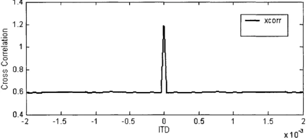
cross-correlating the signals received in the two ears. Identical signals would produce one peak

in the center of the function (figure 1-1), similar to where the image is heard by the

1 .4 I I I I I I 1.2 - xcorr 0 0 0 CO 0.8 0 0.6 0.4 ,iii -2 -1.5 -1 -0.5 0 0.5 1 1.5 2 ITD _x10

Figure 1-1: Summary cross-correlation of 1 second of binaural white noise

individual. If decorrelation is introduced, the width of that peak will broaden. If the

signal is delayed in one ear, the function will represent that circumstance with the peak

shifted over by that delay. In the instance when an individual is presented with two

independent sources, shifted by opposite delays (such as +400 psec and -400 psec), the

function has two peaks present at the two delays (figure 1-2a below).

Two peaks predict that a listener should hear two images: one towards the right

ear and one towards the left. As the figure 1-2b shows, this situation should not change

as exposure to the stimulus continues over time. However, changes seem to occur.

Initially, the stimulus appears as two images, but after some seconds, the two images

appear to merge in the center of the head. If both sources are presented simultaneously,

and continue concurrently, the images merge almost immediately, and the transition from

7 I I I I I - xcorr C 6 - original delay 0 CD 0 C) 0 0 4

3I

I -2 -1.5 -1 -0.5 0 0.5 1 1.5 2 ITD X 10-3

Figure 1-2a: Summary cross-correlation of two statistically independent binaural sources at +400 psec and -400 psec.

Temporal Cross-correlation 6 wD4 2 0 -2 -1.5 -1 -0.5 0 0.5 1 1.5 2 ITD x 10

Figure 1-2b: Temporal cross-correlation diagram of two statistically independent binaural sources at +400 psec and -400 psec taken across a period of 5 seconds.

two images to one is difficult to track. However, if an onset is introduced, where one source begins slightly before the second, the transition is very apparent.' In both cases, the two images lose their individuality while a central image seems to develop. This phenomenon is obviously not demonstrated in the figure 1-2b.

Although the cross-correlation model provides a clear and convenient method of representing certain aspects of lateralization, it does not provide an explanation for this

subjectively observed phenomenon. The purpose of this study was to explore methods of objectifying and characterizing these observations. Typically, it has been easier to investigate the lateralized position of an image rather than its spatial attributes, such as fusion or compactness, and the fact that we are interested in how these attributes change over time does not simplify the matter. Two methods of investigating and quantifying theses changes were attempted. Both focused on the temporal aspects of the

phenomenon, mainly stimulus duration and intersource delay (ISD). This report touches only lightly on the first experiment, since it was dismissed in its early stages, and focuses on the second, as well as on further related studies.

Background

The purpose of this section is to provide the reader with some background information on binaural perception in order to facilitate understanding of the work performed here. The section briefly touches on a variety of areas, some more interrelated than others, but all very relevant. Beginning with a single source in an anechoic

environment, it covers stimulus characteristics, headphones v. a free field environment, different types of subjective impressions, interaural resolution, an example of slow adaptation, and finishes with models of binaural phenomena, more specifically, cross-correlation models.

A Single Source in an Anechoic Environment

Consider first a single source in an anechoic environment, where anechoic is defined as a space free of echoes, reverberation, and ambient noise. This type of acoustic environment simplifies the subject's task in making directional judgments and the

investigator's task in studying and analyzing various questions concerning certain auditory phenomena.

Judgments of direction, distance, and spatial extent are based on both monaural and binaural cues, as well as on the motion of the head. For example, in the case of direction, pinna shape contributes a monaural cue, which can assist in determining whether a source is in front of or behind the listener, while interaural time and intensity differences help determine whether it is towards the left or the right. Moving the head will alter both of these cues since this motion causes a change in propagation path from the source to the ear. As expected, any information gathered from other sensory

mechanisms (e.g., sight) or apriori knowledge will also influence a subject's ability to make these types of judgments.

Stimulus Characteristics

If Y(o) represents the complex spectrum of the acoustic waveform at the

eardrum, and X(o) represents the complex spectrum of the waveform at the source, then Y(o)=X(o))H(o,,). Here, o represents frequency, 0 and * represent source angles, and H represents the transfer function associated with the path from the source to the

eardrum, assuming the source is in the far field. H is normally referred to as the head-related transfer function or HRTF. In the monaural case, it is difficult to determine the values of 0 and

4

without some apriori information regarding X(co) or H. In the binaural case, however, interaural differences can be found by comparing YL(w) for the left ear with YR(O) for the right (i.e., YL(O)/YR(O) = HL(o,0,4)/ HR(o,OJ)).2 These interaural

differences, which change as a function of source position, help determine the values of 0 and

4.

If a sound source is closer to one ear than the other, it goes without saying that there will be a difference in distances between the source and those ears. This imbalance will cause a time delay between when the signal reaches one ear with respect to when it reaches the other. There will also be an imbalance in the intensity level since signals that must propagate around the head to reach the ear will lessen in intensity. In other words, there will always be interaural differences if the source is not located on the median plane.

For purposes of simplicity, it is useful to approximate the head by a sphere with apertures at opposite sides of the diameter representing the ears. Elevation and azimuth

are coordinates for specifying the direction of a sound source relative to the center of this sphere. Azimuth is given by the angle 0 from the median plane, and elevation is given by the angle 8 from the horizontal plane. When describing the position of a source, in most cases, the reference will be with respect to azimuth and the median plane. Interaural time differences (ITDs) and interaural intensity differences (IIDs) are binaural cues that

provide the listener with

Cones of Confusion

important information concerning the location of a sound source; more specifically, they identify a "cone of

confusion" (figure 2-l)3. The +

largr

1TD

surface of the cone is the locus of

smaller

ITD

or

lI1D

_{Figure 2-1}

sources producing the same

interaural time difference and interaural amplitude difference, assuming a spherical head model that ignores near-field effects. Smaller ITDs indicate a location on a broad cone. Larger ITDs indicate a location on a narrow cone. Head movement permits additional discrimination with respect to where a signal is on this cone.

Headphones v. Free-field

Before moving onto spatial impressions something should be said for the difference between headphones and a free-field environment, especially since the

experiments described in this study were conducted over headphones. Using headphones

3 Wenzel, Elizabeth M., Durand R. Begault. "Figure 3.lb. Illustration of the cones of confusion." The Role ofDynamic Information in Virtual Acoustic Displays,

provides the ability to adjust and manipulate ITDs and IIDs exactly and independently. In addition, HRTFs can be easily incorporated into a signal presented through a headset and therefore, the presence of an externalized source can be simulated. Headphones also allow for cases of natural and unnatural stimuli, meaning, the subject can be exposed to a stimulus over headphones he or she would ordinarily never experience in a free-field environment. For instance, they permit the choice of presenting either identical or independent noise to the ears and completely independent noise presented to each ear would be an example of unnatural stimuli. Another example would be opposing time and intensity differences where the signal to one ear leads in time while the signal to the other ear has a higher intensity.

Subjective Impressions

(Fusion, Lateralization v. Localization, Image Shape & Time-Intensity Trading)

When listeners hear a binaural stimulus, they receive two separate signals, one in each ear. These signals may or may not be identical. For instance, an ITD or an IID can be introduced in the left ear making the signal slightly different than the one received in the right. Yet, the listener recognizes only one entity. This is called binaural fusion.

If a source image appears outside the head, it is considered "externalized." If it appears inside the head, it is considered "internalized." Localization is the process of determining the location of a sound source when the image appears outside the head. Lateralization is the process of determining image position within the head, along the interaural axis. ITDs and IIDs can be used to manipulate these positions. Certain factors such as anechoic head-related transfer functions (HRTFs), spatial transfer functions and head movements contribute in allowing a listener to externalize a sound source. Studies

show that adjusting these factors allows for the manipulation of where the image appears to a listener independent of whether the actual source is presented over headphones or over speakers.

With broadband noise, interaural time and intensity differences have particular effects on the movement of the source image. As the IID increases, the source image moves closer to the ear receiving the signal with the higher intensity until it no longer moves but remains by that ear. With an increasing ITD, the source image behaves differently. Instead of remaining at the ear with the leading signal, the image will become wide with respect to both ears. In other words, past a certain ITD, the listener will no longer hear one compact image, but something wide and diffuse, of the type heard when each ear is presented with a statistically independent noise source.

Time-intensity trading describes an empirical phenomenon which claims that for every position along the azimuth defined by a time difference, there is a corresponding intensity difference with the same effect. Equivalence occurs when a listener adjusts the ITD or IID in order to indicate the equivalent position caused by the other. Cancellation occurs when a listener adjusts either in order to counteract the effect of the other. For instance, if an IID causes the sound image to appear to the right of center, the listener can adjust the ITD to move it back to center. Studies indicate the possibility that the listener hears two images since trading ratios between the right and left ears may be different.

Interaural Resolution

Interaural resolution is characterized in terms of minimum audible angle (MAA) and just noticeable differences (JNDs). MAAs describe a listener's ability to determine the direction of a source with respect to a particular reference plane and angle (e.g.,

median plane at 0' elevation). They can change with different source locations. JNDs describe a listener's sensitivity to changes in ITDs and IIDs. Depending on the type of signal and the bandwidth, differences will exist between high and low frequency performance when distinguishing particular time and intensity JNDs.

Slow Adaptation

The binaural system has been shown to adapt slowly to changes in a particular listening situation. In other words, when changes in a listening environment occur, the system's method of processing will not adapt immediately to the new listening

parameters. "Temporal sluggishness" describes the limitation of the system to respond to fluctuations in ITD or IID. Evidence shows that "fluctuations more rapid than about 5 Hz cannot be discriminated from statistically decorrelated stimuli."4 When fluctuations are too rapid to be tracked they lead to a broadening of the image the listener hears.

An example of the system's inability to adjust immediately to changes in an auditory environment has to do with echo suppression. Echo suppression is defined as a "listener's failure to hear the echo as a separate auditory event at its true location."5 Echo threshold is defined "as the shortest delay between lead and lag onsets at which the echo is perceived as a separate sound."5 It can be affected by the "auditory context" such as prior and ongoing stimulation.

The precedence effect is viewed as a "convenient" suppression of echoes allowing the listener to "sort out" the original source from its reflections. At short delays, the

4 Colburn, H. Steven. "Computational Models of Binaural Processing." Auditory Computation, Ed. Harold L. Hawkins, Teresa A. McMullen, Arthur N. Popper, and Richard R. Fay. 11+ vols. New York: Springer-Verlag, 1996.

5 Clifton, Rachel K. and Freyman, Richard L. "The Precedence Effect: Beyond Echo Suppression." Binaural and Spatial Hearing in Real and Virtual Environments, Ed. Robert H. Gilkey, and Timothy R.

listener will detect only one sound while any reflections (i.e., echoes) would "'color' the original sound and reinforce its loudness... At long delays echoes are perceived as separate sounds at their true locations."6 Studies show that a listener's expectations can

affect whether he or she hears the echo and that the ability to suppress echoes changes if the direction or point of origin of the echo changes while the stimulus continues. Instead of registering the echo from a switched direction as a reflection fused with the direct source, the listener registers it as a separate sound source. After some additional

exposure to this new listening scenario, he or she will again be able to suppress the echo and hear only one source, the direct source.

Models of Binaural Perception

Although the auditory system has been a topic of investigation for a long time, there is no model yet available that can account for all types of auditory behavior. The models of binaural hearing that we are most concerned with in this study are those that include some sort of cross-correlation mechanism. The cross-correlation mechanism is ideal in that it can account for both fusion and lateralization and tends to be consistent with the Jeffress model, a neural network where the coincident stimulation of cells relates

interaural delays to the perceived position of the sound source. Cross-correlation looks for similarities using a point-to point comparison of waveforms generated by each ear's stimulus. In other words, it can describe the ability of the auditory system to create an image from complex inputs by selecting the signal components that are common to both ears. The benefit is that cross-correlation accurately represents ITDs and the affect they have in image position. Unfortunately, the mechanism is not as adept at representing the 6 Clifton, Rachel K. and Freyman, Richard L. "The Precedence Effect: Beyond Echo Suppression." Binaural and Spatial Hearing in Real and Virtual Environments, Ed. Robert H. Gilkey, and Timothy R.

effects of IIDs since the cross-correlation function uses the product of the amplitudes of the two stimuli it compares, and therefore, does not have a method by which it specifies which has the greater intensity. It has been suggested that, in this scenario, monaural

cues assist the binaural system in processing the affects of intensity. Many models have additional "mechanisms" which account for the effects of IIDs.

Experimental Setup & Methods

The experiments conducted in this study attempted to characterize the changes in spatial images that seemed to occur over time when two statistically independent white noise sources were presented simultaneously over headphones. Two approaches were devised. In both, the interest lay in changes over time. The first approach focused on the apparent diffusion of the two separated images. The second, and the one ultimately pursued in this study, investigated the possible appearance of a central, merged image resulting from the diffusion. Both experiments were designed as two-alternative forced-choice paradigms to make the task of the subject as simple as possible.

Early Experiments

The first set of experiments were designed to explore the affects of various parameters on the time it takes for the images of two statistically independent noise

sources, lateralized at different positions in the head, to merge, assuming they did in fact merge. First, one noise source was presented at a particular lateral location within the head. At five seconds, a series of shifts in lateral location were introduced into the source

by incrementing or decrementing the interaural time difference (ITD) by some chosen value (e.g., 100 psec). Then, after another selected period of seconds, the second noise source was presented. Conducted as a discrimination experiment, the subject's task was to identify the direction of the lateral shift, for each of 50 shifts. Expected results would show that the subject's accuracy was affected negatively by the second source. The ability to discriminate would deteriorate further as a function of time, after the second source was introduced. This would both demonstrate evidence that there was indeed

some type of diffusion, and perhaps give some indication of how immediately the transition occurred.

The stimuli for these experiments were created with Matlab. Sound sources were generated and combined for each ear since the signal at one ear can be a sum of

waveforms of many individual signals arriving at that ear. Although initial runs of the experiment focused on shift size, the experiment itself was designed to test other parameters such as the primary locations of the two sources, the inter-source delay, and the individual rise-times of the sources.

Each test was configured and administered using a PC with a Pentium processor. The stimuli were presented over headphones, and the subject responded through use of the 1 and 2 (marked as - and +) buttons on a q-terminal. A Matlab GUI interface provided visual cues to prompt the subject's response and supplied right-or-wrong feedback based on the answer.

In pilot tests, ITDs of +200 ptsec and -200 psec defined the location of the two independent sources. Various pilot subjects were tested over a series of shift values from 50 psec to 200 psec to determine a range of shift values over which percent of correct performance exhibited substantial variation. The subjects were exposed to 10 runs per

shift value.

As one would expect, average results showed that at lower shift values, the distribution of correct and incorrect answers tended to be random, whereas at high shift values the answers tended to be completely correct. The range where a set of answers displayed neither random nor completely correct behavior varied from subject to subject. In addition, for most pilot subjects, initial runs showed evidence of lower accuracy than

later runs, demonstrating training effects. Some slight decreases in accuracy occurred, however, they seemed more a result of a distraction due to the introduction of the second source rather than the result of any type of diffusion, especially because the accuracy seemed to improve immediately afterwards. There was no evidence of a gradual change over time and subject fatigue made it impossible to determine whether incorrect answers were indeed a result of the perceived image diffusion. Due to inconclusive results, this course of experiments was dismissed.

Current Experiment

The second approach involved a comparison of two different stimuli. The

purpose was to establish a t= time

Formula A: _{i= ITD (interaural time delay)}

quantitative method of describing YL(t) = N1(t+i) + N2(t+d) d= ISD (inter-source delay) YR(t) = N1(t) + N2(t+d+i) YL(t)= signal at the left ear

the spatial auditory image that the YR(t)= signal at the right ear

listener experiences for different NI(t)= I" noise source

N2(t)= 2"d noise source durations of time. The target stimulus is similar to the previous

stimulus in that it is two statistically independent binaural noise sources delivered concurrently, whose images are spaced equidistant in lateral location from the median plane. This is achieved through the use of ITDs of equal and opposite magnitude (refer to i in the equations of Formula A stated above). The sources were presented either simultaneously (d=0), or with a chosen onset (d>O).

The second stimulus, named the alpha stimulus, is composed of three statistically independent noise sources: one common to both ears, one solely to the left ear, and one solely to the right ear. The power level of the common source is proportional to the positive square root of some modifier a, and the power level of the left and right sources

is proportional to the positive square root of 1 -a when I>cc>O (refer to the equations in Formula B). The correlation coefficient of the right ear and left ear waveforms is a, and the energy to the two ears is independent of a. This produces a set of alpha stimuli such that when w=O the image appears broad and concentrated off to the sides, while when cX=1, the image appears compact and centered at the median plane. The alpha stimulus was devised to simulate the possible different stages of the target stimulus during the transition from two widely spaced images to one central merged image. Unlike the

Formula B: YL(t)= signal at the left ear YR(t)= signal at the right ear YL(t) = Ia"2

1 Ne(t) + I(1-a)12₁ N LIt) Nc(t)= common noise source YR(t) =

1ac

1121 Nc(t) + I(1-a)'12I NR(t) NL(t)= left noise source

NR(t)= right noise source cm= modifier constant where

O:cc1

impression of the target stimulus, the impression of the alpha stimulus remains stable and unchanging independent of duration. It is assumed that for a given duration, the spatial image of the target stimulus will appear similar to some small sub-range of samples within a set of alpha stimuli. It was anticipated that for different durations of target stimulus, the small sub-range of samples would be different; for a shorter duration, the corresponding sample range would be closer to w=O, and for a longer duration, the range would be closer to (x=1.

Pilot versions of the experiment began as a matching paradigm where the subject used a simple audio device such as Wave Player to compare samples of target stimuli with random samples of alpha stimuli and indicate which of the comparisons sounded the

most similar. Pilot runs of this experiment found consistent ranges of alpha values for particular durations.

The experiment then evolved into a comparison paradigm where the question asked was "which noise (stimulus) is wider?" Of course the most crucial parameter of interest was the target stimulus duration. Assuming the spatial impression the subject would remember would be the one the subject experienced last, it seemed logical to take samples of the target stimulus for different lengths of time. What was the subject's spatial impression of these simultaneous noise sources after 0.5 seconds? After 2 seconds? After pilot testing, four durations were selected: 0.5, 1, 2, and 4 seconds. It was found that anything shorter than 0.5 seconds duration made it difficult for the listener to process the spatial properties of the target

stimulus. An alpha stimulus length of one second Target stimulus = 8 types

0 sec intersource delay

was chosen because it provided the subject with just 0.5 sec duration

enough time to register the spatial impression of the I sec duration

2 sec duration

alpha stimulus. This length was maintained 4 sec duration

throughout the study. 0.5 sec intersource delay

0.5 sec duration

The second parameter tested was the delay 1 sec duration 2 sec duration

between the moments the two sources were _{4 sec duration}

introduced, the inter-source delay (ISD). When the

sources began simultaneously (ISD is 0 sec), the diffusion and merging of the two sources seems almost immediate, and the actual transition is harder to observe. An ISD of 0.2 seconds also seemed to have this property. With an ISD of 0.5 seconds, actual movement from two separate images to one central merged image was experienced.

Eleven values of a were chosen for the experiment. They varied from 0 to 1 in increments of 0.1. This set of alpha stimuli was chosen because it covered the whole range of target stimulus stages, not just the transition. A resolution smaller than 0.1 seemed less likely to reveal anything useful.

The stimuli were presented: target stimulus first, then the alpha stimulus. This order was chosen to ensure that the subjects used their final impression of the target stimulus as the image they compared with the alpha stimuli that followed. The time between the presentation of the target stimulus and the alpha stimulus was arbitrarily chosen to be 0.2 seconds. This duration was sufficiently long to allow a clean comparison of two auditory stimuli and sufficiently short to allow the listener to remember both spatial impressions.

The entire experiment was designed and administered utilizing an AMD AthlonTM processor running Windows 2000. Matlab v.6.0 was the software of choice in both preparing the sound (.wav) files and running the experiment. Scripts were written to

generate two independent binaural white gaussian noise sources incorporating the selected ITD (in this case, +400 jsec and -400 Isec) and then to combine the sources using ISDs of 0 and 0.5 seconds to produce the target stimulus.

The alpha stimulus samples were also prepared with Matlab. Three statistically independent monaural white gaussian noise sources were created. One source, the common source, was made binaural with no ITD and saved as a binaural (.wav) file. The left and right sources were then combined and saved as another binaural (.wav) file. The waveform in the common source (.wav) file and the waveform in the left and right

sources (.wav) file were adjusted by different values (0 tol in steps of 0.1) of a and 1-ct

respectively to produce the set of alpha stimuli (refer to Formula B).

A Matlab script also administered the experiment using a GUI interface as the visual cue, and Sennheiser HD270 Control Studio Monitoring Headphones to deliver the stimuli. The response tool was a Logitech optical mouse. There were seven subjects, each of which had normal hearing: one female and six male, four experienced listeners and three inexperienced listeners. All experiments were conducted in a soundproof booth in two sessions spaced out over a period of two weeks.

In each of the two sessions, the subject participated in two experiments, one for each of the two ISDs (i.e., 0.5 and 0 seconds).

Structure:

4 experiments /1I subject For each experiment a set of four tests (for 2 0.5 sec ISD experiment four target source durations) were conducted 2 0 sec ISD experiment with a set of three runs each, and each run 4 tests 1 1 experiment _{contained a set of 22 trials (i.e., comparisons} 3 runs I test

of the target stimulus and alpha stimulus).

22 trials / I run

Figure 3-1 shows a quick breakdown of this Figure 3-1 _{experimental structure, and the following} paragraphs give detailed descriptions of each level in the structure beginning with the trials and working up to the sessions.

Each Trial:

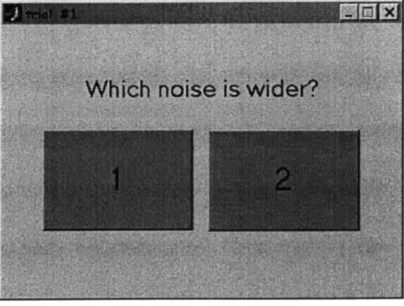
On each trial, the subject was exposed to the target stimulus, then the alpha stimulus. A visual cue, a box with two buttons (figure 3-2), appeared and prompted a choice between the 1' and 2nd stimulus. The subject chose which stimulus appeared

spatially wider by clicking on the corresponding button. It was a two-alternative forced choice between the target (1)

stimulus and the alpha (2nd) stimulus. The target stimulus varied in length depending on which test was being conducted, but the alpha stimulus was always 1 second long and there was

Figure 3-2

always a 0.2 second interval between

the two stimuli in a particular trial. The program moved immediately to the next trial as soon as the subject chose an answer and clicked one of the buttons.

Each Run:

A total of eleven different alpha stimulus segments were used. In order to provide the subject two trials for each alpha segment, every run had 22 trials. The trials were delivered in random order, without replacement, determined at the beginning of each run. This allowed the order to vary from run to run.

Each Test:

Each test investigated the effect of a particular type of target stimulus. For each test, there were three runs with identical target stimulus parameters. Since a particular

test was conducted twice (once/session), there were six runs total for each type of target stimulus.

Each Experiment:

There were four tests per experiment. The length of the target stimulus changed from test to test (0.5, 1, 2, 4 sec). The order of the tests in each experiment differed

-between sessions and across the different subjects in an attempt to overcome ordering effects.

Each Session:

Each subject participated in two sessions with two experiments per session. There was one experiment for the 0 sec ISD target stimulus, and one experiment for the 0.5 sec ISD target stimulus. The subject performed the same two experiments during the second session, but in reverse order. The purpose of spreading both types of experiments over multiple sessions was to take advantage of training effects. A fresh subject can be expected to have trouble adapting the first time through an experiment. The second exposure should be less novel and result in a more efficient performance.

Prior to beginning the first session, the subjects were told that they would be comparing segments of white noise, that they should observe the spatial characteristics of that noise (i.e. the width), and that they needed to pay attention to their last impression of the target stimulus. They were warned that in some of the experiments, the sources in the target stimulus may not begin together, but one after the other. Most importantly, they were informed that there was no "right" answer and that their response should be a true representation of their subjective impression whenever possible.

A preliminary script was run to familiarize the subjects with the different lateral positions a source image could take as well as the different source widths. Examples of a left, right and centered binaural source image were presented as well as of a narrow and wide source image. Finally, the subject was briefly exposed to the eleven alpha segments in ascending order.

A short sample run was administered to acquaint the subjects with the form and rhythm of the experiments as well as the visual, auditory and tactual interfaces. If the subjects were satisfied, they could continue on with the experiment, however, if the subjects remained uncomfortable with the experimental format or the delivery, they had the option of repeating the sample run. The decision to allow the subjects to retake the sample runs arose from the observation that an inexperienced listener might have a harder time adjusting to the experimental procedure, and that this problem might distract the listener from paying attention to the actual experiments. Although no poll was taken to determine how many times each subject ran through the sample run, informal questioning revealed that most subjects ran through it once.

A break was suggested in the middle of each session between the first full

experiment and the second one. During the first session, almost none of the subjects took breaks, however throughout the second sessions almost all the subjects took the offered break. Each session lasted a total of 1 to 11/2 hours.

As stated before, subjects furnished their responses by clicking the mouse on the button that represented the wider stimulus, 1st (target stimulus) or 2 nd (alpha stimulus). A

click on the I" button stored a "1" in the preset answer array, otherwise, a "2" was stored. Each of these answers was stored with the value of alpha presented in the trial, for 22 trials. Since the alpha segments were presented in a random order, the data needed to be

sorted at the end of a run. The new array was a 3 by 11 array; one row for the 11 alpha values, one row to store how many times the target stimulus was chosen and one row to

store how many times the alpha stimulus was chosen over 22 trials. The data was then saved in a ".mat" file.

Data Analysis & Discussion

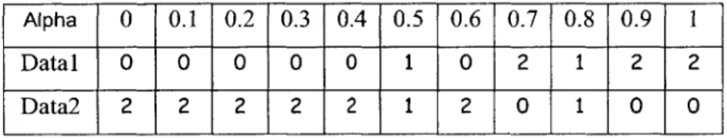
Once the raw data for a particular run was sorted, it took a form similar to that shown in figure 4-1.8 Data] presents the number of times the target stimulus was

selected for a particular value of alpha, and Data2 presents the number of times the alpha stimulus was selected. Since each run had a total of twenty-two trials, two for each value of alpha, the values in Data] can only be 0, 1 or 2. The same is true for Data2. Since the values in Data] and Data2 must always sum to 2 (responses per value of alpha), only

Data] was needed to perform subsequent processing and analyses.

Alpha 0 0.1 0.2 0.3 0.4 0.5 0.6 0.7 0.8 0.9 1

Datal 0 0 0 0 0 1 0 2 1 2 2

Data2 2 2 2 2 2 1 2 0 1 0 0

Figure 4-1: Example of a table of data values for a particular run.

Four possible durations were tested for each inter-source delay (ISD). The data for each duration was gathered over six runs and averaged. With two trials per value of alpha per run and six runs per duration, twelve responses contributed to the averages, as well as to the standard deviation and mode calculations.

Figure 4-29 displays a comparison of the four durations. As expected, most of the data points fall at lower averages for low values of alpha and end at high averages for high values of alpha, confirming that samples with alpha values close to 0 appeared wider

than the target stimulus and samples with alpha values close to 1 appeared narrower than

Subjects A and B, 0.5sec ISD 2 Legend: Duration(sec) 1. - ,-- SubjA 0.5sec S1.5 0 - SubjA isec C. SubjA 2sec SubjA 4sec -- - SubjB 0.5sec 0-- -- - - SubjB isec 120 -SubjB 2sec 0 --- --- SubjB4sec 0 0.1 0.2 0.3 0.4 0.5 0.6 0.7 0.8 0.9 1 alpha

Figure 4-2: This chart presents a comparison of data collected over four durations. The different texture in lines represents data from two different subjects. The ordinate axis ranges from 0 to 2 and represents the total possible average of responses over 6 runs. Each of the eleven values of alpha (0...1) is displayed along the abscissa.

the target stimulus.'

0

For middle values of alpha there is a transition where subjects

began to experience a degree of uncertainty in deciding whether the target stimulus

appeared wider than the alpha stimulus. The overall shape is something between a

diagonal line and an s-shaped curve depending on the particular subject.

Based on the assumed spatial width behavior of the target stimulus one would

assume that a target stimulus of duration

0.5

seconds would appear wider than a majority

of the alpha stimulus and thus begin to transition earlier than a target stimulus of duration

4 seconds. It follows that for the ascending duration values of the target stimulus, the

areas of transition would be spaced apart across the ascending range of alpha values; the

lines corresponding to shorter durations closer the left of the graph and the lines

corresponding to longer durations closer to the right. The data in figure 4-2 clearly do

not exhibit these expectations. In fact, no particular or recognizable order seems to exist

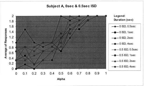
Subject A, Osec & 0.5sec ISD 2 Legend: 1.8 Duration (sec) 1.6 -+-0 ISD, 0.5sec 1.4 -n- 0 ISD, 1sec

a

1.2 - 0 ISD, 2sec 1-.-- 0 ISD, 4sec 0

~

0. -*-0.5 ISO, 0.5sec 0.6 > 0.

~n0.5

ISO, 1sec 0.2 0 .5 ISD, 2sec 0 -00.5 SD, 4sec 0 0.1 0.2 0.3 0.4 0.5 0.6 0.7 0.8 0.9 1 Alpha

Figure 4-3&4: Each of these two figures represents a particular subject. They contain the data from both ISDs superimposed. The different color in lines represents an ISD of 0 seconds and an ISD of 0.5 seconds. All four durations are displayed. The ordinate axis ranges from 0 to 2 and represents the total possible average of responses over 6 runs. Each of the eleven values of alpha (0... 1) are displayed along the abscissa.

Subject B, Osec & 0.5sec ISD 2

1.8 Legend:_{Duration (sec)}

1.6

U)

O 1.4 -- 0 ISD, 0.5sec

C

a.

1.2 -u--0 ISD, 1sec

A1

-&-0

ISD,

2sec 0

U) 0.8 --- 0 ISD, 4sec

0.6 -+- 0.5 ISD, 0.5sec

< 0.4 -u--0.5 ISD, 1sec

0.2 -- 0.5 ISD, 2sec

0 -- 0.5 ISD, 4sec

0 0.1 0.2 0.3 0.4 0.5 0.6 0.7 0.8 0.9 1 Alpha

with these data. Nor is there any other type of behavior specific to one duration or to one subject.

As stated in the "Experimental Setup and Methods" section, the effects of two different ISDs (0 and 0.5 seconds) were investigated in this study. 0.5 seconds was chosen because it seemed to produce the most observable transition from two separate images to a central image. 0 seconds was chosen because its effects would be expected to mimic the effects of an indefinite duration. In other words, it served as a type of control. Based on this premise, one would expect little change in data over the different durations for an ISD value of 0 seconds.

Figures 4-3&4 show comparisons of the data collected for each ISD over the different durations. Each figure represents the data from a particular subject." Since little change is expected over the durations for an ISD of 0 seconds, the transition areas of the four durations should fall relatively close together. The transition areas for 0.5

seconds should appear spaced out following the trends mentioned earlier. It is apparent that the data does not adhere to these expectations for either of these subjects. Instead the transition areas appear equally random for both ISDs.

However, when the data for six of the seven subjects is averaged together, the results appear closer to expectations. Each data point in figures 4-5&6 are the average of 72 responses. In these figures, the transitions for the Osec ISD fall almost on top of each other while the transitions for the 0.5sec ISD are relatively spread out. However there still seems to be little significance in the order of the 0.5sec ISD lines, and the lines are close enough to be argued that they too fall almost on top of each other.

Average of Answers where Target Stimulus Was Found Wider for Osec ISD

2 1.8 m 1.6 o 1.4 a-0 -. 5sec cn 1.2 -in-1sec E .2sec to 0.8 -- 4sec ) 0.6 0-0. S 0.2 0 0 0.1 0.2 0.3 0.4 0.5 0.6 0.7 0.8 0.9 1 Alpha Values

Figure 4-5&6: These figures contain the averages the data for each ISD over all the subjects. All four durations are displayed. The ordinate axis ranges from 0 to 2 and represents the total possible average of responses over 6 runs. Each of the eleven values of alpha (0.. .1) are displayed along the abscissa.

Average of Answers where Target Stimulus Was Found Wider for 0.5sec ISD

2 1.8 1.6 o 1.4 u 1.2 -e-.5sec -i-1sec E 2sec 0.8 -..- 4sec 0 0n 0.6 0.4 ( 0.2 0 0 0.1 0.2 0.3 0.4 0.5 0.6 0.7 0.8 0.9 1 Alpha Values

Although the figures 4-2,3 and 4 only show the data from at most three different subjects, none of the subjects exhibited evidence of the expected trends.1 2 Yet there seem to be some differences among subjects with respect to those who were experienced listeners and those who were not 3_{. Experienced listeners seemed to have cleaner data;}

for lower alpha values the average responses seemed to be less than .4, the transitions were relatively linear, and for higher alpha values the average responses seemed higher than 1.8. Inexperienced listeners produced data a little less consistent. Traditionally, the first few data points were erratic, especially for the 0.5 second duration, however this is also the case for one of the experienced listeners.1 4 _{In figure 4-2, subject B was}

experienced, while subject A was not. Similarly, figures 4-3&4, subject B is experienced and subject A is not. Aside from one subject15 in particular, the rest did experience the

general transition of narrower to wider as the alpha values increased.

Finally a comparison was also made between performances between sessions since three of the six runs were presented in session 1 and three in session 2. Therefore, averages for a particular duration and ISD were calculated for a particular session. As figure 4-716 shows, for some subjects, the performance did improve from one session to the next. Although not completely consistent throughout all seven subjects, it appears to be the case for the majority. This would be expected, as the style of the experiment included no alteration in the format, and subject training would be expected.

12 _{Graphs for the rest of the subjects found in Appendix A}

13 Subjects 1, 3, and 5 were inexperienced, subjects 2, 4, 6 and 7 were experienced. 14 Subject 2's data shows an irregularity at (x=3 for: ISD Osec, Dur _{0.5 sec.}

15 Subject 5 _{expressed difficulty in determining which stimulus was wider for any of the values of alpha,}

and the data supports the conclusion that subject 5 could not hear the differences in spatial attributes and was therefore incapable making any type of comparisons. Subject 5's data is located in Appendix A-1.

Subject Com p Dayl/Day2, .5sec ISD, .5sec Dur Figure 4-7: This figure

represents a comparison

2.00 between _{" and 2 d session}

1.80 averages for a particular

1.60 duration and ISD. The blue

1.40 line represents the data from

s 1.20 session and the pink line

k 1.00 aylavg represents the data from session

-- D a y 2 ag _2. 0.80 0.60 0.40 0.20 0.00 0.00 0.10 0.20 0.30 0.40 0.50 0.60 0.70 0.80 0.90 1.00 Alpha

Since the transition areas exhibited linear characteristics, further analysis was

conducted in which trendlines were fit to the data in these areas. Then, based on the

slope of these lines, the alpha value where the target stimulus was found wider for

50%

of the responses was calculated. The slopes themselves can reveal how clearly the

subject perceives the spatial width of the sources; a steeper source indicating a fast

transition from when the target stimulus appears narrower than the alpha stimulus to

when it appears wider. A more level slope demonstrates uncertainty. This uncertainty

can indicate a broader source image or simply increased difficulty for the listener in

making the comparison.

Excel was used to plot the data and estimate the trendlines based on the points in

the transition area. First, the ordinate values, originally from 0 to 2, were converted to

percentages. Instead of an average response value to a particular alpha value, the points

would represent the percentage of responses that found the target stimulus wider. Two

sets of rules were then devised in order to choose which points to include in the linear

estimation. The first set decided the lower alpha cut-off value and the second set decided the higher alpha cut-off value.

Lower rule: First, the highest alpha value yielding

Lower alpha formula:

a percentage of 10% or lower (8.3% or 0%) was x lss=l

x=x(greatest) for which y(x)<10%

found. If the alpha value directly before it yielded a (if does not apply, x=x(greatest) when

lower percentage, it was chosen. If not, the first y(x) is lowest)

until xless=O,

was chosen. If there was no percentage of 10% or if _x=x-1y(x-_)<Y(x) else

lower, the highest alpha value yielding the lowest x-less=0 end

available percentage was chosen. x.begin=x; The higher rule is identical to the lower rule, but in reverse.

Higher rule: First the lowest alpha value yielding a

Higher alpha formula:

xfmore=1 percentage of 90% or higher (91.7% or 100%) was

x=x(lowest) for which y&)>90%

(if does not apply, _{found. If the alpha value directly before it yielded a} x=x(lowest) when

y(x) is greatest)

higher percentage, it was chosen. If not, the first was

until xmore=O,

if y(x+1 )>y(x) _{chosen. If there was no percentage of 90% or higher,} x=x+1

else

x_more=O _{the lowest alpha value yielding the highest available} end

x_end=x;

percentage was chosen.

For both rules, there is an extra stipulation for the case in which there are no points with percentages below 10% or higher than 90%. This was added to take advantage of sets of data where there was a lower phase, a transition phase, and higher phase, but the lower or higher data points did not fall within the specified cut-off areas.

Once it was determined which points to use, trendlines were computed and slopes with intercepts were recorded. These were graphed with the full set of points for each

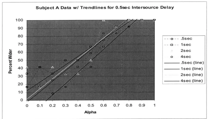
Subject A Data w/ Trendlines for 0.5sec Intersource Delay 100 90 80 -- +b-- .5sec 70 --- 1-- 1sec a 60 2sec o 4sec 50.5sec _(line) 41sec (line) 30 2sec (line) 4sec (line) 20 10 0 0 0.1 0.2 0.3 0.4 0.5 0.6 0.7 0.8 0.9 1 Alpha

Figure 4-8&9: These figures represent the data for two different subjects, one experienced and one inexperienced. The data points are connected by the dotted line, while their trendline is solid in the same color. Four durations are displayed. The ordinate axis ranges from 0 to 100 and

represents the percentage of responses where target stimulus was chosen for a particular alpha. Each of the eleven values of alpha (0... 1) are displayed along the abscissa.

Subject B Data w/ Trendline for 0.5sec Intersource Delay 100 90 80 -8- .5sec 70 --- a-- isec 60 2sec --- o-- 4sec 50 _ .5sec (line) 4 40 1sec (line) 30 2sec (line) 4sec (line) 20 10 0 0 0.1 0.2 0.3 0.4 0.5 0.6 0.7 0.8 0.9 1 Alpha

duration. Figures 4-8&9" exhibit the data for two subjects for 0.5sec ISD. None of the

trendlines for any of these subjects demonstrate any type of effect that can be associated with changing duration.

Using the linear equations given by the trendlines, the alpha values at the 50% mark were then calculated. Both the slopes and the 50% alpha values were plotted against the four durations for every subject (Figure 4-10&11). Although only two are shown here, four graphs were plotted, two for the 0 sec ISD and two for the 0.5 sec ISD'8. Ideally the alpha value for the 50% mark would increase across duration. The slope on the other hand might be expected to decrease, however, none of the graphs exhibit consistent trends among the subjects that would suggest any kind of affect based on duration.

Almost every analysis performed on the data failed to reveal any kind of identifiable effect that could be associated with the parameters tested. An ANOVA analysis was conducted on the slope values and on the 50% values, to evaluate whether there were any significant differences between the groups of data.19 The analysis was

carried out across duration, for every subject, for both ISDs. The results of this analysis failed to show any significant (p=0.01) differences with respect to duration or ISD.

17 _{Data taken from Subjects 1 and 4.} " These graphs are available in Appendix A

Linegraph of Duration v. Slope over Subjects for 0.5sec Intersource Delay 6 5 --- Subject 1 4 -u- Subject 2 Subject 3 .23 - Subject 4 -*- Subject 5 2 -e- Subject 6 --- Subject 7 1 0

0.5 sec 1 sec 2 sec 4 sec

Duration (sec)

Figures 4-10 & 11: The upper graph displays the change in slope as a function of the target stimulus duration. The lower graph displays the change in alpha values where the target stimulus was found wider than the alpha stimulus 50% (0.5) of the time. Both of these graphs are for the target stimuli with the 0.5 second ISD.

Alpha values at the 50% mark for the four durations (0.5sec Intersource Delay 1 0.9 0.8 -+- Subject 1 007I --n- Subject 2 0.6 _{Subject 3} w 0.5 -x- Subject 4 C0.4 -w- Subject 5 0.3 -- Subject 6 --- Subject 7 0.2 0.1 0

0.5 sec 1 sec 2 sec 4 sec

Conclusions

This study originated with the observed diffusion of the images of the two

simultaneous statistically independent noise sources. Experiments were designed to test

the hypothesis that when the two sources, separated by some onset, were presented, the

amount of diffusion and merging perceived would increase as a function of the duration

of the stimulus. Unfortunately, the data yielded very little evidence to support this. A

possible effect of inter-source delay (ISD) that was suggested by the grouping of all

subjects together produced no statistical significance in the ANOVA study.

Certain factors that could have contributed some unreliability in the data include:

undetected errors in the stimuli or format of the experiments, inadequate preparation of

the subjects, insufficient testing of the subjects, or subject fatigue. It seems unlikely,

however, that such effects would constitute a primary cause of our negative results.

Perhaps a more plausible reason that the data did not demonstrate any support for

the hypothesis was that the question asked was misleading. In the experiment, the

instructions ask the subject to decide "which (of the two stimuli) is wider." This question

is based on a particular interpretation of the observed phenomenon. Initially, when two

separate source images are perceived, one on the right and one on the left, the impression

is considered "wide." When the separate images begin to diffuse and a central image

emerges, the impression is considered "narrow." The question of "which noise is

wider?" inherently assumes that the listener will observe that central image and

eventually lose track of the separate images as the diffusion continues. A possible error

in this assumption suggests that although the subjects would observe that central image,

they may still be rather aware of the original separated images despite the diffusion. In

fact, the diffusion of the two images could conceivably prompt a "wider" decision. One method to correct this might be to instruct the subjects to focus on the median plane and describe the width of the noise they hear with respect to that focal point.

Possible support for these concerns regarding the diffused presence of the two noise sources was found when re-examining figures 4-5&6. Trendlines were

approximated and slopes were calculated for the transition areas.20 Figure 5-1 shows a table of the linear equations ISD Duration Trendline Equations

calculated. All four slopes for 0.5 seconds y = 2.6091x - 0.5605

0 1 second y = 2.6488x - 0.6081 the 0 second ISD are virtually _{seconds 2 seconds y = 2.5794x - 0.5278}

equivalent. For the 0.5 second 4 seconds y = 2.6389x - 0.5417

ISD, it seems like there might be 0.5 seconds y = 2.9444x - 0.8444 0.5 1 second y = 2.7679x - 0.5575

some inverse relationship seconds 2 seconds y = 2.629x - 0.4147 between the slopes and the 4 seconds y = 2.4405x - 0.3611

Figure 5-1: Table of the linear equations calculated for the

duration of the target stimulus. data averaged over all the subjects. These numbers support the part

of the hypothesis that claims that diffusion does occur over time. As stated before, a shallow slope indicates more uncertainty in judging the spatial characteristics of the images. The two noise sources were presented at +400 tsec and -400 ptsec, and although this would make them appear "wide", together they should still appear narrower than the alpha stimulus when wc=0 (i.e., completely uncorrelated noise is presented to the two ears). Yet, if the two images become diffuse, they might appear to spread in both

20 _{For the 0 second ISD, the slope was calculated over the range of a (0.4 to 0.9) and for the 0.5 second} ISD, the slope was calculated over the range of a (0.4 to 0.9 for dur =0.5 seconds and 0.3 to 0.9 for dur =1,2 & 4 seconds ). Actual graphs can be found in Appendix A-6.

directions allowing the overall impression to appear wider instead of narrower with increased duration. By this reasoning, subject confusion would be understandable when interpreting the spatial impression of the diffusion and merging of the separated noise sources.

At this point, only two possible conclusions can be stated. Either there is no such phenomenon and those listeners who observed it were mistaken, or the experimental design was flawed in that it did not provide the subjects with adequate instructions and tools in order to appropriately observe and interpret the phenomenon. We believe the latter is more likely and that, indeed, the wrong question was asked. Although individual subject data did not follow the expected trends, analysis of the data as a whole has hinted at possible effects by duration and ISD. Therefore, it cannot be said that the data truly refutes the existence of the phenomenon. The results of this study are inconclusive and further investigations must be carried out in order to give some objective dimension to the elusive phenomenon observed.

Recommendations for Future Research

The first step in investigating the apparent diffusion of the separate source images was to find some way of substantiating the subjective reports of the phenomenon's existence. Up until this point, there was no prior research aimed specifically at this phenomenon, and the only evidence available was the testimony of the listeners based on their individual spatial interpretations. The experiments in this study were geared

towards objectifying the phenomenon by finding a quantitative method of characterizing it.

Although the current study did not produce the expected results, it has not been fruitless. It provided an environment for developing strategies that might be valuable in the search for an improved experimental design. Along these lines, new alternatives for examining the diffusion of the source images have been formulated.

One way to change the experiment would be to ask the subject whether or not the target stimulus seems similar in spatial characteristics to the alpha stimulus (as a function of cc). Another way would be to ask the subject to rate the similarity since some subjects will always find the target and alpha stimuli similar, and other subjects will never find them similar. The rating scale could range from 0 to 10 where 0 means there is no

similarity, and 10 means the two stimuli sound identical. The rest of the experiment format would remain the same, including the presentation of the two stimuli and the GUI interface, which the subjects originally used to answer the question. If the rating question were used, the GUI interface would have ten buttons instead of two. Overall, both methods might pose a simpler perceptual question for the subjects than the one asked in the experiments actually performed ("Which noise is wider?"). The rating system would