Publisher’s version / Version de l'éditeur:
Vous avez des questions? Nous pouvons vous aider. Pour communiquer directement avec un auteur, consultez la
première page de la revue dans laquelle son article a été publié afin de trouver ses coordonnées. Si vous n’arrivez pas à les repérer, communiquez avec nous à [email protected].
Questions? Contact the NRC Publications Archive team at
[email protected]. If you wish to email the authors directly, please see the first page of the publication for their contact information.
https://publications-cnrc.canada.ca/fra/droits
L’accès à ce site Web et l’utilisation de son contenu sont assujettis aux conditions présentées dans le site LISEZ CES CONDITIONS ATTENTIVEMENT AVANT D’UTILISER CE SITE WEB.
AWWA 2004 Annual Conference [Proceedings], pp. 1-16, 2004-06-01
READ THESE TERMS AND CONDITIONS CAREFULLY BEFORE USING THIS WEBSITE.
https://nrc-publications.canada.ca/eng/copyright
NRC Publications Archive Record / Notice des Archives des publications du CNRC :
https://nrc-publications.canada.ca/eng/view/object/?id=6b2c09de-5f5a-4fdb-962f-64f0d9e41079 https://publications-cnrc.canada.ca/fra/voir/objet/?id=6b2c09de-5f5a-4fdb-962f-64f0d9e41079
This publication could be one of several versions: author’s original, accepted manuscript or the publisher’s version. / La version de cette publication peut être l’une des suivantes : la version prépublication de l’auteur, la version acceptée du manuscrit ou la version de l’éditeur.
Access and use of this website and the material on it are subject to the Terms and Conditions set forth at Alternative strategies for pipeline maintenance/renewal
Alternative strategies for pipeline maintenance/renewal
Rajani, B.; Kleiner, Y.
NRCC-45353
A version of this document is published in / Une version de ce document se trouve dans : AWWA 2004 Annual Conference, Orlando, Florida, June 13-17, 2004, pp. 1-16
ALTERNATIVE STRATEGIES FOR PIPELINE
MAINTENANCE/RENEWAL
Balvant Rajani, Senior Research Officer and Yehuda Kleiner, Group Leader, Senior Research Officer
Institute for Research in Construction
National Research Council of Canada, Ottawa, Ontario, Canada K1A 0R6
ABSTRACT
This paper addresses decision-making issues faced by most water utilities regarding their water mains. An overview is provided to explain the difference between failure
management of small-diameter mains in distribution systems and failure prevention in large-diameter transmission pipelines. The paper further describes past and on-going research at the National Research Council of Canada (NRC) on these issues. A description is provided for the application of fuzzy logic to assess failure risk of large diameter
transmission pipelines. Case studies are described to illustrate the application of a multi-variate time-exponential model to historical failure rates in small-diameter distribution mains. The impact of time-dependent factors on water main breaks is demonstrated, with special emphasis on the effect of various cathodic protection measures on the life-cycle costs of water mains.
INTRODUCTION
This paper addresses decision-making issues faced by most water utilities regarding their water mains, namely, (1) failure management of mains in distribution systems vs. failure prevention in large transmission pipelines, (2) application of fuzzy logic to assess failure risk of large diameter transmission pipelines, and (3) the effectiveness of cathodic protection of distribution systems illustrated through the application of a multi-variate time-exponential model. These issues are discussed in the context of possible strategies for effective management of pipeline maintenance and/or renewal.
In the following discussions the terms rehabilitation, renewal, and replacement are simply referred to as renewal for the sake of brevity. The few references provided were selected to demonstrate the points made, and constitute only a fraction of the relevant body of work that is available in the literature.
In this paper, a case is first made on why it is important to address failure prevention of large transmission pipelines and manage failures of small diameter mains. This discussion is followed by on how failure risk of large diameter transmission pipelines can be assessed where there is a dearth of data on pipeline condition state, as well as a poor understanding of the behavior and performance of existing pipelines. Finally, case studies are presented to
illustrate the application of a multi-variate time-exponential model to historical failure rates in small-diameter distribution mains. The impact of time-dependent factors on water main breaks is demonstrated, with special emphasis on the effect of various cathodic protection measures on the life-cycle costs of metallic water mains.
Mathematical and modelling details have been omitted because essential details are
published elsewhere and in order not to overwhelm and distract the reader from the overall discussion on alternative strategies for pipeline maintenance/renewal.
THE CHALLENGE OF MAKING DECISIONS ON WATER MAIN RENEWAL A balance between system performance and costs is the essence of decision making on the renewal of infrastructure systems. It is widely accepted that performance criteria for water distribution networks must include quality, quantity and reliability components. More specifically, the water should be safe, with acceptable aesthetics, taste and odour; regular and peak demand (including fire flows) should be met with acceptable pressure and with minimal interruptions.
The costs involved in a water distribution system comprise capital investment in system design, installation and renewal, operation and maintenance (energy, materials, labour, monitoring, inspection, repair) and indirect and social costs resulting from failure (property damage, disruption, illness, etc.).
What makes the decision process so challenging for water mains is: mechanisms affecting the performance criteria are not well understood; it is difficult to define and measure performance, let alone decide what level of performance is acceptable; it is difficult to calculate the costs involved to achieve a specific level of performance; and the collection of data on the performance and condition of these buried assets is difficult and costly. Add to these the spatial and temporal variabilities inherent in even a moderate-size system, and one might begin to understand the magnitude of the difficulty in providing a holistic decision framework.
Failure risk in a water distribution network
The failure of a distribution system is broadly defined as the inability (momentary or extended) to meet any of the performance criteria discussed above. As pipes age they deteriorate, resulting in increased failure frequency. In the context of reliability
engineering and risk management, the definition of risk depends on the type of asset or system (Henley and Kumamoto, 1981). For buried pipes one can define the risk of any type of failure as the expected magnitude of the consequences of failure(s), i.e.,
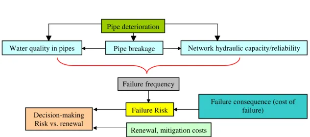
Figure 1 depicts the authors’ view of the general framework for making comprehensive decisions regarding the renewal of water distribution systems.
Fig. 1. A general framework for decision making in water distribution system.
Probability of Failure (failure frequency)
The probability of failure can be assessed in different ways, some more rigorous than others, depending on the type of failure and on the available data.
The probability of a water main failure due to structural deterioration can be estimated using physical (mechanistic) models (Rajani and Kleiner, 2001) and/or statistical models (Kleiner and Rajani, 2001). Statistical models develop empirical relationships between the pipe, its exposure to the external and operational environments and its observed failure frequency while physical models mimic realistic field conditions as well as external and operational environments. However, a lot of the data required to represent these conditions and environments are either unavailable or very costly to obtain for even a modest portion of a distribution network, primarily because of spatial variability. These empirical models typically over-simplify a complex reality in order to achieve “80% of the answer with 20% of the effort”.
The availability of fast and robust water network simulation programs has facilitated the ability to calculate the probabilities of hydraulic failures. However, difficulties still remain with issues such as calibration of roughness coefficients, modelling and predicting demand variations, and modelling and predicting the deterioration of roughness coefficients due to tuberculation and corrosion and their spatial and temporal variations.
The probabilities of water quality failures in distribution systems have yet to be addressed in a rigorous manner. There are numerous ways (Kleiner, 1998; Sadiq et al., 2003) in which water quality failures can occur including: (a) intrusion of contaminants, (b)
regrowth of micro organisms, (c) microbial (and/or chemicals) breakthrough, (d) leaching of chemicals or corrosion products, and (e) permeation of organic compounds. The
complexity of the mechanisms leading to some of these failures, exacerbated by the spatial and temporal variabilities in the physical state of the pipes as well as the systems’
boundary conditions (physical environment, efficacy of treatment, etc.) makes direct physical modelling very challenging. An on-going research project, co-funded by the
Pipe deterioration
Network hydraulic capacity/reliability Water quality in pipes Pipe breakage
Failure frequency
Decision-making Risk vs. renewal
Failure consequence (cost of failure)
Failure Risk
American Water Works Association Research Foundation (AwwaRF) and the National Research Council of Canada (NRC) is attempting to meet these challenges, using techniques that combine field data with expert opinion.
Consequence (Cost) of Failure
The costs of a water main failure event may be classified into three categories: (a) direct, (b) indirect, and (c) social costs. While direct costs are relatively easy to quantify in
monetary terms, indirect costs may require much more effort, and social costs are often the most difficult to describe and assess. Rajani and Kleiner (2002) summarized the details on specific items within each category.
Hydraulic and water quality failures that are not related to pipe structural failure result in costs that are mainly indirect or social costs, e.g., loss of production, fire extinguishing, quality of life, etc. It can be said that generally, one cannot spot-repair a hydraulic or a water quality failure in the same manner that a ruptured pipe is repaired. A hydraulic and a water quality failure usually points to deficiencies that have to be addressed on a wider scale, such as cleaning, scrubbing, lining (non-structural) or out-right replacing various components of the network. Operational changes (e.g., ortho-phosphate) are required in some cases. In the context presented here, the cost of these remedies are not considered as failure costs, but rather as renewal (lining, replacement) or maintenance (flushing, ortho-phosphate) costs.
The magnitude of failure consequence is, strictly speaking, a random value because no two failures have the same consequences. Failures in small distribution mains are usually repaired with little effort and typically collateral damage is relatively small. Failures of large transmission mains are relatively rare, and because only few water utilities attempt to assess total failure damage there are currently insufficient data to assign probability
distributions to failure costs. The consequences of hydraulic failures are rarely assessed, except when fire liability is concerned. The consequences of water quality failures receive increasing attention because of media exposure, but rigorous assessments are yet to be published. More research is required to gain a better understanding of the true magnitude of indirect and social consequences of all failure types.
Risk of Failure
Risk mitigation can be achieved by reducing both probability and/or the cost of failure, as risk depends on both (equation (1)). As was stated earlier, the probability of failure increases as the distribution system ages and deteriorates. In some cases, it can be argued that the cost of failure is also likely to increase over time, for example, when a pipe is located in a rapidly developing area, but generally it is assumed that failure cost is not time-dependent.
Measures to mitigate risk from the cost side are possible but rather limited in scope, e.g. timely response by a well-trained pipe repair crew will reduce the cost of repair as well as water loss and collateral damage resulting from a main break; a good monitoring program will detect low quality or unsafe drinking water and thus enable faster communication to
the public of any water safety failure, thus minimizing the level of exposure; an adequately sized storage tank can reduce the vulnerability of a hospital to a hydraulic failure.
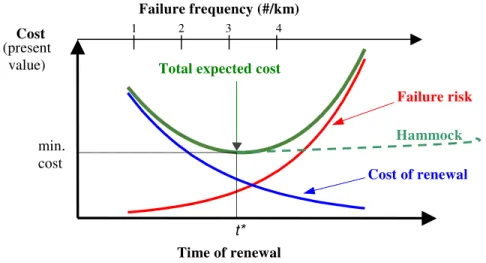
It appears that mitigating risk on the failure frequency side has a greater potential because theoretically, one can reduce failure frequency to nearly zero (thus reducing risk to nearly zero) albeit at a very high cost. It follows that a rigorous decision process should find a balance between the risk of failure and the cost to mitigate it. Fig. 2 illustrates how this balance varies over time. As long as the pipe continues to age and deteriorate without renewal, its probability of failure (or failure frequency) increases and the risk increases as well (note that here the risk is expressed in discounted expected cost). At the same time, the discounted cost (or present value) of pipe declines as its renewal is delayed.
The total expected life-cycle cost (sum of the total expected cost of failure and cost of renewed pipe) typically forms a convex shape, whose minimum point depicts the optimal time of renewal (t*). The curve depicting total cost in Fig. 2 is deeply convex with a clear minimum point at t*. This is a rather idealized case, which may change in some cases. When ageing rate (i.e., the rate at which failure frequency increases) is similar in
magnitude to the discounting factor, the convexity of this curve can become quite flat, and the point of minimum cost becomes less crisp. When the cost of failure is relatively low compared to the cost of renewal and the discounting factor relatively high, the curve can take the shape of the “hammock-chair” as described by Herz (1999), with no definite minimum, indicating that renewal could perhaps be postponed indefinitely.
Fig. 2. Deciding when to renew a water main with a low cost of failure.
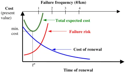
As the consequences (or cost) of failure increase, so does the failure risk, pushing the failure risk curve (Fig. 2) higher. Fig. 3 illustrates a case where failure cost is significantly higher, resulting in a typically elevated total cost curve, with a minimum point (t*) shifted much to the left. The top horizontal axis of the graph in Figs. 2 and 3 indicates the failure frequency corresponding to the time of renewal. While in Fig. 2 the failure frequency at t* is about 3 events per unit length per unit time, in Fig. 3 this frequency is reduced to less than 1. Figs. 2 and 3 illustrate that failure management is a typical strategy for relatively
Time of renewal
(present
value) Total expected cost
min. cost t* Cost Failure risk Cost of renewal Failure frequency (#/km) 1 2 3 4 Hammock
small diameter distribution mains with low failure cost, while failure prevention is appropriate for large water transmission mains, with relatively high cost of failure.
Fig. 3. Deciding when to renew a water main with a high cost of failure.
With regard to structural failures, when the cost of failure is relatively low and failure frequency can be tolerated, it is often (but not always) sufficient to rely on empirical models using historical breakage patterns to predict future failure rates. However, high failure costs may justify the use of extra measures to anticipate failures and prevent them in a pro-active approach. These measures could include inspection and condition
assessment using non-destructive evaluation (NDE) techniques in conjunction with
physical/mechanical models. As the costs of NDE techniques decrease, the justification for applying them to small pipes with low cost of failure will also increase.
It should be emphasized that the life-cycle cost curves depicted in Figs. 2 and 3 are qualitative and idealized. True costs are often hard to come by and are subject to large variations, as are true deterioration rates. Consequently, determination of the optimal time for renewal (t*) requires many simplifying assumptions.
RISK ASSESSMENT OF LARGE-DIAMETER TRANSMISSION MAINS
As discussed earlier, large transmission mains typically have low failure rates but when they fail the consequences can be quite severe. This low rate of failure, coupled with high cost of inspection and condition assessment, have contributed to the current situation where most municipalities lack the necessary data to model the deterioration rates of these assets and subsequently to make rational decisions regarding their renewal.
The condition assessment of a large transmission main comprises two steps. The first step involves the inspection of the main using direct observation (visual, video) and/or non-destructive evaluation (NDE) techniques (radar, sonar, ultrasound, sound emissions, eddy currents, etc.), which reveal distress indicators. The second step involves interpretation of these distress indicators to determine the condition state of the main. This interpretation
Time of renewal
(present value)
Total expected cost
min. cost t* Cost Failure risk Cost of renewal Failure frequency (#/km) 1 2 3 4
process is dependent upon the inspection technique. Interpretation of the visual inspection results, although based on strict guidelines, can often be influenced by subjective
judgment. The interpretation of NDE results on the other hand, is often complex (at times proprietary) and imprecise.
Managing the failure risk of large transmission mains requires a deterioration model to enable the forecast of the asset condition as well as its possibility of failure in the future. Significant research effort has been carried out in the last two decades to model
infrastructure deterioration. The Markov deterioration process (MDP) is one approach that has gained prominence as exemplified by Madanat et al. (1997), Kleiner (2001) and others. Examples of other types of statistical models include Lu and Madanat (1994), Ramia and Ali (1997), Flourentzou et al. (1999), Ariaratnam et al. (2001) and others.
In recent years, increased research effort has been dedicated to the application of soft computing methods to assess infrastructure deterioration. Soft computing methods include techniques such as artificial neural network (ANN), genetic algorithms (GA), belief networks (BN), fuzzy sets and fuzzy techniques. Fuzzy techniques seem to be particularly suited to model the deterioration of buried infrastructure assets for which data are scarce and cause-effect knowledge is imprecise. Consequently, The NRC is engaged in the development of a promising approach to assess risk of transmission pipelines that combines the advantages of both the Markov deterioration process and fuzzy logic. Fuzzy Sets
A fuzzy set describes the relationship between an uncertain quantity x and a membership function which ranges between 0 and 1. A fuzzy set is an extension of the traditional set theory (in which x is either a member of set A or not) in that an x can be a member of set A with a certain degree of membership. Fuzzy techniques help address deficiencies inherent in binary logic and are useful in propagating uncertainties through models.
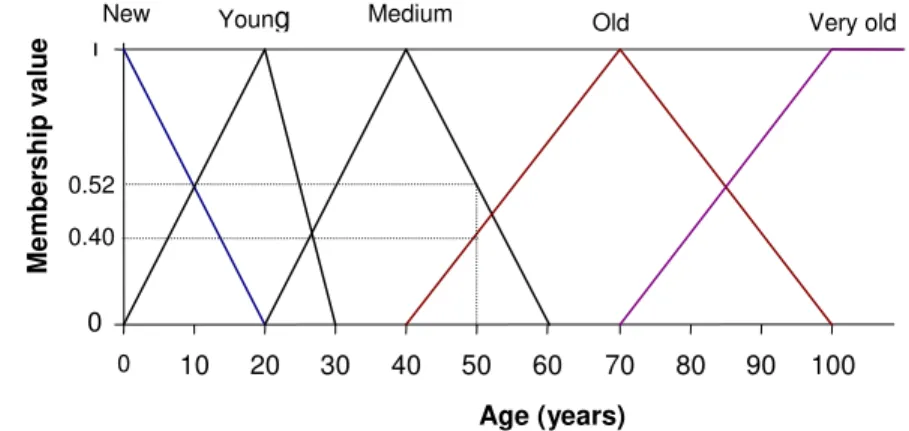
Membership functions are often represented by triangular fuzzy numbers (TFN), which permit the use of linguistic variables (Lee, 1996). To illustrate the concept, suppose that the age of a pipe is defined by five fuzzy subsets (or numbers), each representing an age
grade; A1 = “new”, A2 = “young”, A3 “medium”, A4 = “old” and A5 = “very old”, as
illustrated in Fig. 4. The fuzzy subset A3 “medium” for example, has a membership
function such that for age x below 20 years or above 60 years the membership to “medium” is zero, and for age between 20 and 60 years the membership follows straight lines that
form a triangle. Fuzzy set A comprises the collection of the five subsets (or numbers) Ai.
Further, a crisp (exact) pipe age can be mapped onto the fuzzy set A so that it has memberships of 0.52 and 0.4 to age grades medium and old, respectively.
Fig. 4. Example of fuzzy sub-sets (numbers).
Fuzzy rules and knowledge base
In fuzzy rule-based models, the relationships between variables are represented by means of fuzzy if-then rules of the form “If antecedent proposition then consequent proposition”. The antecedent proposition is always a fuzzy proposition of the type “x is A” where x is a linguistic variable and A is a linguistic constant term. The proposition’s truth-value (a real number between zero and 1) depends on the degree of similarity between x and A. This linguistic model (Mamdani, 1977) has the capacity to capture qualitative and highly uncertain knowledge in the form of if-then rules such as,
If ‘pipe’ is old and ‘pipe condition’ is good then ‘deterioration’ is slow (2)
A rule set comprising several rules and the linguistic variables that belong to specific sets constitute the knowledge base of the linguistic model. Each rule is regarded as a fuzzy relation and can be applied using several methods such as fuzzy conjunctions (Mamdani method) as described in Mamdani (1977) and Yager and Filov (1994).
The knowledge base that governs the deterioration process is described in detail in Kleiner et al. (2004).
The rule-based fuzzy Markov deterioration process
A Markov process with a discrete state space is called a Markov chain. For example, the state space of pipe condition can be defined by seven states (or grades), excellent, good, adequate, fair, poor, bad, and failed. These grades can be depicted by the notation C1, …,
C7, respectively. The deterioration of a pipe in a Markovian process describes how the pipe
condition transits from state Ci to state Ci+ 1. Traditionally, this transition is done through a
probability function, which is the conditional probability of a transition from state Ci to state
Ci+ 1 during a given period of time. As it deteriorates through many time periods, the
probability of the pipe being in the more deteriorated states gradually increases.
0 1 0 10 20 30 40 50 60 70 80 90 100 Age (years) Memb er ship valu e
New Young Medium Old Very old
0.40 0.52
In the fuzzy Markov process, which is under development, membership values to the various states are used rather than probabilities. As the pipe deteriorates, memberships
“flow” from state Ci to state Ci+ 1. The transition process is governed by a set of rules
(rather that transition probabilities as in the traditional Markov process), which is constructed based on expert opinion (Kleiner et al. 2004).
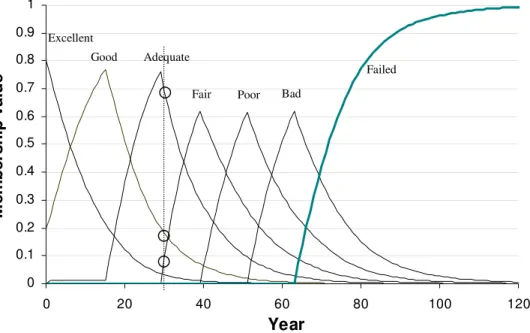
The training (or calibration) of the fuzzy Markov deterioration model to a given pipe, requires at least one observation (or inspection) of the pipe at a time that is sufficiently later than the time of installation. For example, immediately after installation (when time t = 0), a pipe is assumed to have been in a condition state represented by the fuzzy set
C0 = (0.9, 0.1, 0, 0, 0, 0, 0) meaning 0.9 membership to excellent, 0.1 membership to good
and zero membership to all other condition states. At age t = 30 years an inspection and condition assessment were carried out and the pipe’s condition was determined to be
C30 = (0, 0.2, 0.7, 0.1, 0, 0, 0), meaning 0.2 membership to good, 0.7 membership to
adequate, 0.1 membership to fair and zero memberships to all other condition states. The resulting deterioration curves are as illustrated in Fig. 5.
Fig. 5. Example deterioration curves.
Once deterioration curves are determined they are used to estimate the time in the future when the pipe is expected to approach the failed state. The deterioration model can be re-calibrated with each additional inspection and condition assessment.
Any pipe inspection, whether visual, NDE or other reveals evidence about the existence and extent of distress indicators on the pipe. These distress indicators have to be
interpreted and translated into the fuzzy condition state space described earlier in this section. A condition assessment framework for translating the distress indicators into fuzzy condition states is described in detail by Kleiner et al. (2004).
0 0.1 0.2 0.3 0.4 0.5 0.6 0.7 0.8 0.9 1 0 20 40 60 80 100 120 Year M e mb er sh ip val u e Excellent Good Adequate
Fair Poor Bad
Fuzzy rule-based risk
Risk is a function of both probability of failure and magnitude of consequence as indicated previously in equation 1. In the realm of buried pipes failures, not only is the likelihood of failure difficult to quantify, but failure consequences as well. Therefore, consequences of failure are defined on a fuzzy qualitative nine-grade scale from extremely low to extremely severe. An additional fuzzy rule set is established to govern the risk level obtained from the possibility of failure obtained from the deterioration model and the perceived level of failure consequence. For example, the following can be a rule in this set
If ‘failure possibility’ is medium and ‘failure consequence’ is severe then
‘failure risk’ is quite severe (3)
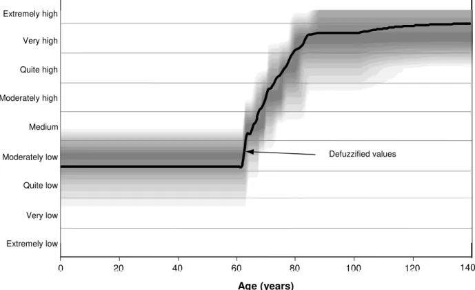
For example, if the failure consequence of the pipe from the earlier example is represented by the fuzzy set S = (0, 0, 0, 0, 0, 0.2, 0.5, 0.3, 0), meaning membership values of 0.2, 0.5 and 0.3 to fuzzy subsets moderately severe, quite severe, and very severe, respectively. The resulting fuzzy risk curve is illustrated in Fig. 6. The intensity of the grey levels represents the membership values to the respective risk levels
Fig. 6. Fuzzy risk levels over the life of a pipe
It should be pointed out that the fuzzy-based approach does not lend itself to a cost-balance analysis illustrated in Fig. 3, because the concept of discounting cannot be easily applied to costs that are expressed in fuzzy linguistic terms. Consequently, the decision on optimal
0 20 40 60 80 100 120 14014 Extremely low Extremely high Very high Very low Quite low Quite high Moderately high Moderately low Medium 0 20 40 60 80 100 120 140 Age (years) Defuzzified values
time of renewal has to be based on maximum acceptable risk levels as opposed to minimum cost (t*).
RENEWAL OF SMALL-DIAMETER DISTRIBUTION MAINS
As previously described, failure in small distribution mains is typically associated with relatively low value consequences. As a result, the decision making process is usually intended to manage or limit failure frequency rather that prevent it. To that effect, the governing approach is to examine historical patterns of increase in failure rates, use those to predict expected failure rates in the future, and then compute the expected life-cycle costs, as in Fig. 2, to determine the best renewal timing.
Numerous approaches have been proposed to decipher historical failure patterns. Kleiner and Rajani (2001) provided a comprehensive review of the major ones, and it appears that more have been published in the last 3 years. In this paper we shall illustrate the general concept of failure management, using work that has been done at the NRC.
Time-dependent factors affecting water main breaks
The multi-variate time-exponential (Kleiner and Rajani, 2002) or the time-power (Mavin, 1996) model attempts to correlate historical repair rates (surrogate for pipe deterioration) with dynamic explanatory variables. It is a simple model that permits the inclusion of a variety of dynamic explanatory variables, e.g., environmental such as soil shrinkage and swelling, annual temperature variations, and operational such as the implementation of corrosion protection, pressure changes, etc.
Climatic covariates for which data are typically available are freezing index and rainfall deficit. Freezing index (FI) is a surrogate measure for the severity of winter, and rain deficit (RD) is a surrogate measure for soil moisture. RD can be considered in two separate forms. Cumulative RD, which is a measure of the average soil moisture over a given time period, corresponds to the effects described by Rajani et al. (1996). Snapshot RD, which is a measure of the soil moisture during winter, when the soil is mostly frozen, corresponds to the effects described by Rajani and Zhan (1996).
The cathodic protection of metallic water mains is a typical operational covariate for which water utilities keep data, if appropriate. Cathodic protection can be defined as “…the reduction or elimination of corrosion by making the metal a cathode by means of an impressed direct current or attachment to a sacrificial anode (usually magnesium,
aluminium or zinc)” (NACE, 1984). In practice, water utilities can implement two cathodic protection strategies, namely, hotspot and retrofit CP. Hotspot CP is the practice of
opportunistically installing a protective (sacrificial) anode at the location of a pipe repair. These anodes are typically installed without any monitoring and stay in the ground until total depletion, usually without replacement. Retrofit CP refers to the practice of
systematically protecting existing pipes with galvanic cathodic protection. If the existing water main is electrically discontinuous (e.g., bell and spigot with elastomeric gaskets and no bridging) then an anode is attached to each pipe segment (typically 6 m or 20’ length).
If the water main is electrically continuous then usually a bank of anodes in a single anode bed can protect a long stretch of pipe.
The effect of time-dependent (operational) factors on life-cycle costs
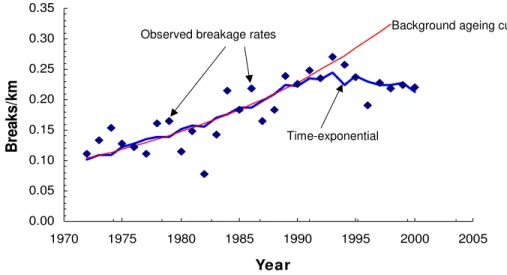
Fig. 7 illustrates how the multi-variate time-exponential model was able to “explain” observed breakage patterns an Eastern Ontario water utility (Utility A). The model was applied to a group of pipes that comprises 634 km of cast iron water mains, 6” (150 mm) to 12” (300 mm) in diameter, installed between 1946 and 1970. Utility A commenced a hotspot cathodic protection program (HS CP) in 1990, in which every pipe breakage repair was followed by an installation of a 32 lb. magnesium anode. These anodes typically provide adequate protection for 15 years. The effect of the hotspot program is clearly visible as predicted breaks begin to deviate from the background ageing curve (indicating theoretical breakage rate if no time-dependent factors were present) in the early 1990’s. Full details on the manner with which the hotspot cathodic protection effect is modelled are provided in Kleiner and Rajani (2004).
Fig. 7. Effect of hotspot CP program on cast iron mains in Utility A.
It should be noted that in this case history, climatic effects on historical breakage rate appear to be minimal and cannot explain the deviations of the observed breaks from the background ageing in the period prior to the hotspot program.
Breakage rate can be predicted and economic analysis can be performed using the
parameters obtained from the application of the time-exponential model. Fig. 8 illustrates how the application of hotspot cathodic protection in Utility A impacts the life cycle cost of small-diameter CI water mains. The total cost curve (as in Fig. 2) is shifted down (to lower total costs) and to the right (to extend the economic life of the pipe by deferring t*).
0.00 0.05 0.10 0.15 0.20 0.25 0.30 0.35 1970 1975 1980 1985 1990 1995 2000 2005 Year B rea ks/ km
Background ageing curve
Time-exponential Observed breakage rates
Fig. 8. Effect of hotspot CP on the life-cycle costs of pipes – Utility A
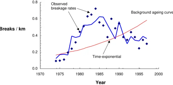
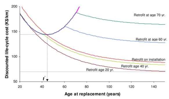
Figs. 9 and 10 illustrates the impact of retrofit cathodic protection. The model was applied to a Southern Ontario water utility (Utility B), which initiated a retrofit CP program in the mid 1980’s on 86 km of 6” (150 mm) to 12” (300 mm) diameter ductile iron mains installed between 1970 and 1987. The downturn in the number of breaks soon after the retrofit program began is clearly visible in Fig. 9.
Fig. 9. Effect of retrofit on ductile iron mains in Utility B.
$40 $80 $120
20 40 60 80 100 120 140
Age (years) at replacement
Tot a l di s c ount e d l if e -c y c le c os ts ( $ K /k m ) Start HS CP on installation Start HS CP at age 40 Start HS CP at age 60 No HS CP t* to * Start HS CP at age 80 Start HS CP at age 100 0.0 0.2 0.4 0.6 0.8 1970 1975 1980 1985 1990 1995 2000 Year
Background ageing curve
Time-exponential Observed
breakage rates
Fig. 10. Effect of retrofit CP on the life-cycle costs of pipes – Utility B.
The impact of retrofit cathodic protection on the life cycle cost of small diameter DI mains in Utility B is illustrated in Fig. 10. Again, in this case retrofit cathodic protection can act to reduce overall life costs as well as defer the optimal time of replacement. Full details on how retrofit cathodic protection was modelled are provided in Kleiner and Rajani (2004). It should be noted that in the case studied presented here the multi-variate time-exponential model was able to fit (or “explain”) the observed data well. There are cases, where the model does not fit quite well, possibly due to quality of data, impact of factors that are not considered, lack of homogeneity in the samples group of pipes or limitations of the model itself.
FINAL REMARKS
In general, the industry seems to be progressing in the right direction despite many challenges and inherent complexities in the management and operations of water supply and distribution systems. Much progress has been made in the understanding of
deterioration processes and failure modes in the last few years. At the same time, as practices change and new materials are used, the knowledge gap, while decreasing from one end is increasing from the other.
As NDE techniques evolve, including the development of various sensors and robots, it appears that failure anticipation and prevention is likely to become more technologically feasible as well as affordable. Currently, it seems that only mains prone to high-cost failure (namely transmission mains) can justify these techniques, but over time this will likely change. In the meantime, while the bulk of water distribution networks are comprised of
50 100 150 200
20 40 60 80 100 120 140
Age at replacement (years)
D is c ount e d l if e -c y c le c os t ( K $ /k m ) Retrofit on installation Retrofit age 40 yr.
Retrofit at age 60 yr.
t*
Retrofit age 20 yr.
small mains with relatively low failure consequence, NDE techniques can, in some circumstances, be used as complementary means to the empirical models, which rely on historical break records.
The scarcity of data on deterioration rates for large-diameter buried pipes, coupled with the imprecise and often the subjective nature of pipe condition assessments merits the use of fuzzy techniques to model their deterioration. The deterioration process is modelled as a fuzzy rule-based non-homogeneous Markov process applied at each time step to arrive at deterioration curves. The consequences of pipe failure are defined on a fuzzy scale with nine intensity grades ranging from extremely low to extremely severe. The level of risk, which is also defined on a nine-grade fuzzy scale from extremely low to extremely high, can then be determined (inferred) based on another fuzzy rule base.
Two case studies have been presented to demonstrate the application of a multi-variate exponential model to the breakage patterns of small-diameter distribution mains. These case studies demonstrate how the consideration of time-dependent factors can help in explaining year to year variations in pipe breakage rates. They also illustrate how in some cases cathodic protection can extend the economic life of pipes as well as reduce their life-cycle costs.
REFERENCES
Ariaratnam, S.T., El-Assaly, A. and Yang, Y. 2001. Assessment of infrastructure needs using logistic models. Journal of Infrastructure Systems, ASCE, 7(4): 160-165. Flourentzou, F., E. Brandt, and C. Wetzel. 1999. MEDIC – a method for predicting
residual service life and refurbishment investment budget. Proceedings of the 8th conference Durability of Building Materials and Components, Edited by M.A. Lacasse and D.J. Vanier, NRC, pp. 1280-1288, Vancouver.
Henley, E.J. and Kumamoto, H. 1981. Reliability Engineering and Risk Assessment. Prentice-Hall, Englewood Cliffs, NJ.
Herz, R. 1999. Bath-tubs and hammock-chairs in service life modelling. Proceedings of the
13th European Junior Scientist Workshop, pp. 11-18.
Kleiner, Y. and Rajani, B.B. 2004. Quantifying effectiveness of cathodic protection in water mains: theory. To appear in Journal of Infrastructure Systems, ASCE, pp. 1-32. Kleiner, Y. 1998. Risk factors in water distribution systems. British Columbia Water and
Waste Association 26th Annual Conference, Whistler, BC, Canada.
Kleiner, Y. 2001. Scheduling inspection and renewal of large infrastructure assets, Journal of Infrastructure Systems. ASCE, 7(4): 136-143.
Kleiner, Y. and Rajani, B.B. 2001. Comprehensive review of structural deterioration of water mains: statistical models. Urban Water, 3(3): 157-176.
Kleiner, Y. and Rajani, B. B. 2002. Forecasting variations and trends in water main breaks. Journal of Infrastructure Systems, ASCE, 8(4): 122-131.
Kleiner Y., Sadiq, R. and Rajani, B.B. 2004. Modelling failure risk in buried pipes using
fuzzy Markov deterioration process. To appear in Pipelines 2004, ASCE, San Diego, CA.
Lee, H.-M. 1996. Applying fuzzy set theory to evaluate the rate of aggregative risk in software development. Fuzzy Sets and Systems, 79: 323-336.
Lu, Y. and Madanat, S.M. 1994. Bayesian updating of infrastructure deterioration models. Transportation Research Record 1442: 110-114.
Mamdani, E.H. 1977. Application of fuzzy logic to approximate reasoning using linguistic systems, Fuzzy Sets and Systems. 26: 1182-1191.
Mavin, K. 1996. Predicting the failure performance of individual water mains. Urban Water Research Association of Australia, Research Report No. 114, Melbourne, Australia.
NACE. 1984. Corrosion Basics – An Introduction. National Association of Corrosion Engineers, Edited by A. deS. Brasunas.
Rajani, B.B. and Kleiner, Y. 2001. Comprehensive review of structural deterioration of water mains: physical models. Urban Water, 3(3): 177-190.
Rajani, B. and Kleiner, Y. 2002. Towards Pro-active Rehabilitation Planning of Water Supply Systems. International Conference on Computer Rehabilitation of Water Networks - CARE-W, Dresden, Germany.
Ramia, A.P. and Ali, N. 1997. Bayesian methodologies for evaluating rutting in Nova Scotia’s special B asphalt concrete overlays. Canadian Journal of Civil Engineering, 24(4): 1-11.
Rajani, B. and Zhan, C. 1996. “On the estimation of frost load.” Canadian Geotechnical J., 33(4): 629-641.
Rajani, B., Zhan, C. and Kuraoka, S. 1996. Pipe-soil interaction analysis for jointed water mains. Canadian Geotechnical J., 33(3): 393-404.
Sadiq, R., Kleiner, Y. and Rajani, B.B. 2003. Forensics of water quality failure in distribution systems - a conceptual framework, Journal of Indian Water Works Association, 35(4): 1-23, Oct/Dec.
Yager, R.R. and Filev, D.P. 1994. Essentials of fuzzy modelling and control. John Wiley & Sons, Inc., NY.