Building Load Control and Optimization
By
Hai-Yun Helen Xing M.S., Building Technology (2000) Massachusetts Institute of Technology
Submitted to the Department of Architecture In Partial Fulfillment of the Requirements for the Degree of
Doctor of Philosophy in Building Technology
at the
Massachusetts Institute of Technology February 2004
© 2004 Massachusetts Institute of Technology All rights reserved
Signature of the author... ...
Department of Architecture January 9, 2004
C ertifie d b y ... .. ... Leslie K. Norford Professor of Building Technology Thesis advisor
Accepted by... ... . ... Stanford Anderson Chairman, Department committee on Graduate Student Head, Department of Architecture
ROTCH
MASSACHUSETTS INSTITUE, OF TECHNOLOGY
cFEB
2 7 2004
THESIS COMMITTEE:
Professor Leslie Norford, Professor of Building Technology
Professor Leon Glicksman, Professor of Building Technology and Mechanical Engineering George Macomber Professor
Building Load Control and Optimization
By
Hai-Yun Helen Xing
Submitted to the Department of Architecture on January 9, 2004 in Partial Fulfillment of the Requirements for the Degree of
Doctor of Philosophy in Building Technology
Abstract
Researchers and practitioners have proposed a variety of solutions to reduce electricity consumption and curtail peak demand. This research focuses on load control by improving the operations in existing building HVAC (Heating, Ventilating and Air-Conditioning) systems and by aggregating individual loads based on optimization studies. Emphasis is placed on electricity rates and climate data in California, where electricity costs have been of particular concern. The optimization problem in this research is multi-objective in the sense that we aim to reduce building load while maintaining an acceptable level of comfort.
The first part of this research focuses on optimizing controls in a single building. A simple three-zone VAV system model is built in EnergyPlus (E+). The cost function structures and the potential difficulties associated with simulation-based optimization are discussed. Discontinuity and nonlinearity are of major concern. Two optimization algorithms are tested and applied to a variety of problems: Direct Search (DS) and Genetic Algorithms (GA). An E+ simulation based GA optimization environment is developed in Matlab. DS is found to be efficient with small problems in this research, while GA works in almost any situation with the price of intensive computation. A few operations guidelines are proposed.
The second part of this research presents three ways of optimizing load control in an aggregation pool: Enumeration, multi-GA and model-based nonlinear optimization. Enumeration relies on expert rules to find a small set of feasible solutions through automated E+ simulations and search exhaustively for the optimal solution. Multi-GA solves the aggregation problem in the Matlab GA environment with sequential E+ simulations as the function evaluator. Because simulation-based optimization is very computationally intensive in handling multiple buildings, the model-based approach develops for each aggregation participant a time series model and several regression models to predict individual load profiles under load control. It then applies an interior-point-method-based commercial solver LOQO to these simplified building models. This system is fast and easy to scale up. Certain precision is lost due to modeling simplifications, but the results are still satisfactory for practice purposes.
Overall, load aggregation offers load diversification opportunities among participants and improves the aggregated load profile. Load shedding later individual load profiles in a way that enhances the aggregation performance.
Thesis Supervisor: Prof. Leslie Norford Title: Professor of Building Technology
ACKNOWLEDGEMENTS
I would like to take this opportunity to thank my advisor Professor Leslie Norford for his insight, guidance and enormous support in the past five years. I wouldn't be able to finish this work without his help. He has always been patient, understanding, and open-minded. He has encouraged me to explore the unknown and to pursue my interest. I am fortunate to have him as the advisor.
I also want to thank my committee members Professors Leon Glicksman and Steve Leeb for their advice. Working with them has been a pleasant experience and their impact on me goes beyond research.
A special thank-you to Phil Haves at LBNL. His encouragement has accompanied me since the Tsinghua years. He also offered valuable advice on load shedding issues in this work.
Many thanks to the California Energy Commission for funding this project. I appreciate the financial support from the Institute in the past five years.
Many colleagues and friends helped me along the way. Michael Wetter at Laurence Berkeley National Lab advised me with great patience on GenOpt and Direct Search. Michael Witte and the EnergyPlus support team helped me debug EnergyPlus code. Colleagues at the MIT Operations Research Center helped me with both course work and my research. Discussions with Henry Spindler
and Peter Armstrong have been helpful and enjoyable. Henry Spindler and Phil Sun offered good suggestions in improving the thesis presentation.
My deepest gratitude goes to my parents and my brother. They are always there for me and never have any doubt. I thank Tony for his love and support, and for going through the difficult times with me.
TABLE OF CONTENTS Abstract 5 Acknowledgements 7 List of Tables 12 List of Figures 14 Chapter 1 Introduction 19 1.1 Introduction 19 1.2 Research overview 20 1.3 Literature research 21 1.4 Problem description 37
Chapter 2 Single Building Simulation-based Parametric Studies on a Simple VAV System 41
2.1 Model description 41
2.2 Model test 45
2.3 Energyplus-based parametric studies - part I 46
2.4 Energyplus-based parametric studies - part II 52
2.5 Another load shedding strategy - night cooling 64
2.6 Single building load control summary 74
Chapter 3 Single Building EnergyPlus Simulation-based Optimization 77
3.1 Direct Search algorithms and GenOpt 77
3.2 Genetic Algorithms and GAOT 81
3.3 Cost function structure 83
3.4 Single building optimization based on Direct Search and EnergyPlus 87
3.5 A GA-based optimizer for single-building study 92
3.6 Algorithm comparison 100
3.7 A hybrid algorithm - future work 100
Chapter 4 Simulation-based Multi-Building Optimization 103
4.1 Smart Enumeration - a Rule Based Engineering Approach 103 4.2 Set thermostat set points for multiple buildings by Smart Enumeration 104
4.3 4.4 4.5 4.6 Chapter 5 5.1 5.2 5.3 5.4 5.5 5.6 Chapter 6 6.1 6.2 Chapter 7 7.1 7.2 References Appendix A A.1 A.2 Appendix B B.1 B.2 B.3 Appendix C C. I
Matching results of a two-building case for night cooling based load control A GA approach to the multi-building problem
Computation concerns of simulation-based approaches Multi-building optimization - economy of scale
A Model -Based Nonlinear Optimization Approach to the Multi-Building Problem Problem formulation
Base load predictor - a time series model Load reduction model
Comfort model
A nonlinear central optimizer
Comparison of three approaches to the multi-building problem
Non-technical Aspects of the Load Control Problem Energy crisis review
Non-technical issues
Conclusions Conclusions Future work
EnergyPlus input file of the base model Core of the EnergyPlus input file
Matlab GA code for both single and multiple buildings GenOpt code
VBA post processing
EnergyPlus key inputs for three models used in the aggregation studies
121 129 135 136 141 141 144 157 162 165 170 171 171 174 179 179 182 185 189 191 202 204 206
C.2 Matlab code for exhaustive search in Enumeration C.3 VBA code for feasibility check in Enumeration209
Appendix D D.1 D.2
SPlus codes for model identification AMPL code of the nonlinear optimizer
206
216 223
LIST OF TABLES
Table Table name and content Page
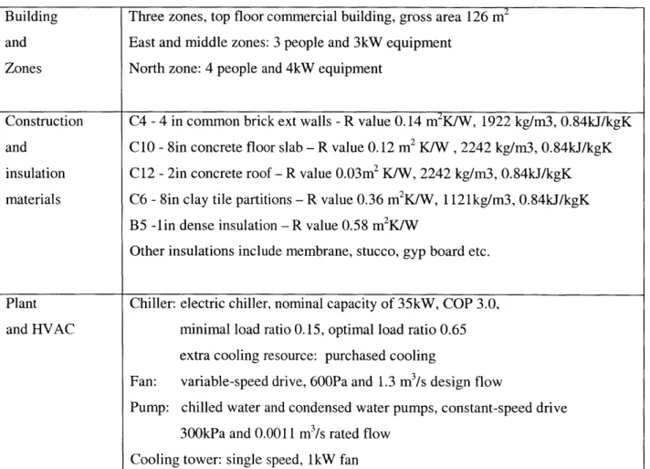
2.1 Basic building model 44
2.2 Demand reduction vs. Load shedding strategies 59
2.3 Night cooling summary 74
3.1 Optimize peak load with different start points through Direct Search 89 3.2 Optimize different objective functions through Direct Search 90
3.3 Example rate structure 89
3.4 Optimize trade-off between energy and comfort through Direct Search 91
3.5 Performance of the Matlab-GA results 100
3.6 Comparison of GA and DS 101
4.1 Building model types used in the multi-building research 105 4.2 Summary of simple thermostat-based aggregation cases 108 4.3 Individual load control vs. aggregated load control 109
4.4 Example rate structure 110
4.5 Summary of simple aggregation cases, cost-based 111
4.6 Individual load control vs. aggregated load control, cost-based 111
4.7 Two EnergyPlus models used for night cooling 123
4.8 Night cooling schedules 123
4.9 Night cooling based load aggregation: peak load and total energy cost 123 4.10 Aggregated night cooling details: contribution by individual participants 124
Table Table name and content Page
4.12 Optimizing two-building night cooling schedules with the Matlab GA -peak 132 load as the cost function
4.13 Optimizing two-building night cooling schedules with Matlab GA- total cost 132 with a $6.5/kW demand charge
4.14 Optimizing two-building night cooling schedules with Matlab GA- total cost 132 with a $1.5/kW demand charge
4.15 EnergyPlus runs taken by multi-GA 136
4.16 Total computation time comparison between Enumeration and multi-GA 136
4.17 Aggregation performance - mix matters 138
4.18 Aggregation performance - economy of scale 138
5.1 Model Coefficients and t- values for building 1 -A first cut 148 5.2 Model coefficients and t values for building 1- with only significant variables 150
5.3 Peak load as a function of exogenous variables 153
5.4 SPlus regression results for load reduction model at different hours 159 5.5 Load reduction model prediction errors in the testing set 159
5.6 PMV model prediction errors in the testing set 165
5.7 Model-based optimizer vs. Enumeration 168
5.8 Aggregation using the model-based approach 169
LIST OF FIGURES
Figure Figure name and content Page
2.1 Floor plan of the three-zone VAV system 42
2.2 Plant layout of the three-zone VAV system 42
2.3 Air loop of the three-zone VAV system 43
2.4 Daytime average chiller, fan, total power, and PPD vary with thermostats 47
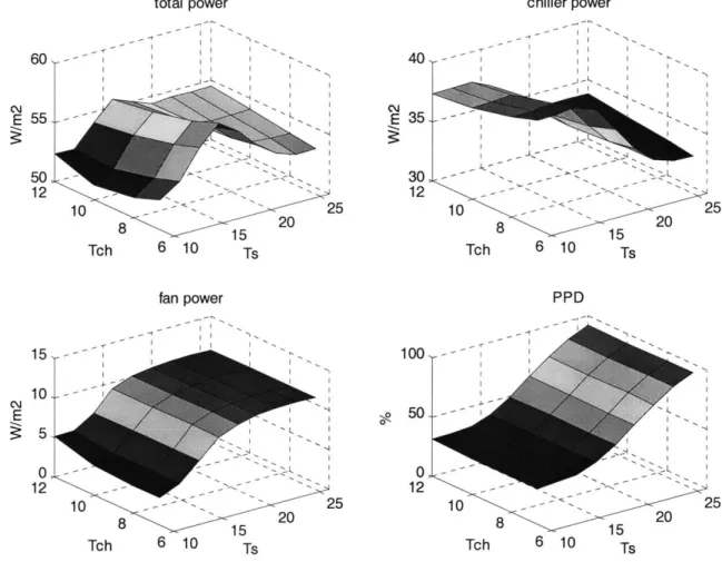
2.5 Total, chiller and fan power, and PPD vary with the combination of supply air 49 temperature and chilled water temperature with the fan capacity fixed at full
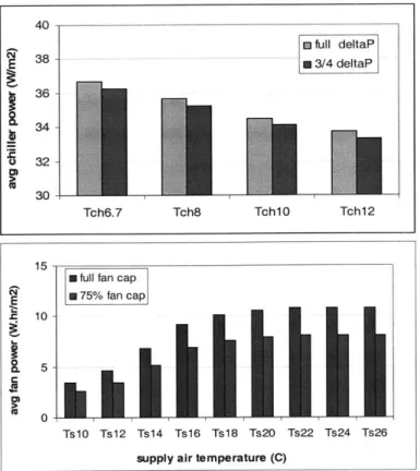
2.6 Chiller power varies with chilled water temperature and fan power varies with 50 supply air temperature, at full and 75% fan capacity
2.7 Total, chiller and fan power vary with combination of supply air temperature 50
and chilled water temperature at full and 75% fan capacity
2.8 Chiller and fan power vary with economizer set points 51
2.9 Power and PPD profiles with hours 14-17 thermostats adjustment 54 2.10 Daytime total and chiller power reductions with different thermostat set points 54
during hours 14-17
2.11 Average total power reductions and contributions by fan and chiller with supply 55 fan capacity reduction and hour 14-17 thermostats adjustment
2.12 Power and PPD profiles with combinations of supply air temperature increases, 57 chilled water temperature increases, and fan capacity reduction
2.13 Average total demand reduction and contributions by fan and pump and by 58 chiller for combinations of supply air temperature increase, chilled water
temperature increase, and fan capacity reduction
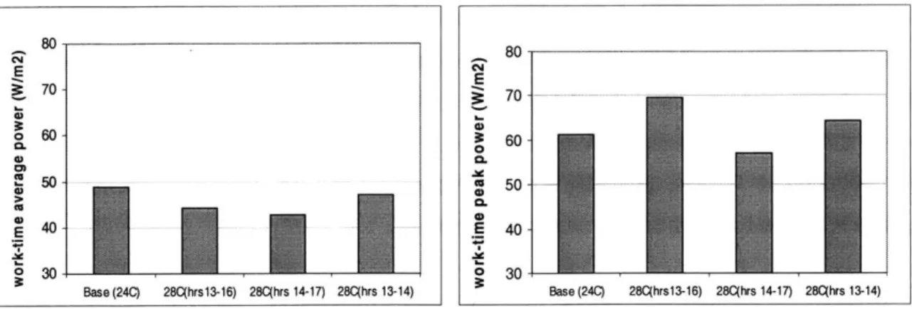
2.14 Daytime average power consumption and peak load with different scheduling 61 durations and starting times under thermostat-based load control
2.15 Power and PPD profiles with different scheduling durations and starting times 61 under thermostat-based load control
Figure Figure name and content
2.16 Average power consumption and PPD for three chiller on/off cases and three 62 types of thermal mass
2.17 Power and PPD profiles vary with thermal mass under temporary chiller-off 63 strategies and load setback recovery comparison between Imass and 3mass
2.18 Load profiles and peak/average load differences of night cooling by mechanical 66 ventilation with different discharging processes
2.19 Load profiles and peak/average load differences of chiller-based night cooling 67 with different discharging processes
2.20 Load profiles and summary statistics of night cooling by mechanical ventilation 70 with different fan starting times
2.21 Load profiles and summary statistics of chiller-based night cooling with 71 different chiller starting times,
2.22 Load profiles of no night cooling, chiller-based and fan-based night cooling, 72 LA and Austin
2.23 Peak load and average load comparison between three thermal mass types, three 73 night cooling strategies and two locations of LA and Austin
3.1 GenOpt overall organization 80
3.2 GenOpt optimizer class 80
3.3 EnergyPlus-based GAOT scheme 82
3.4 Cost function surface of total load varies with hours 16 and 17 thermostats 85
3.5 Cost function surface of PPD varies with hours 16 and 17 thermostats 85 3.6 Cost function surface of peak load varies with hours 16 and 17 thermostats 86 3.7 Power profiles of different scenarios with hours 16 and 17 thermostats as 86
control variables
3.8 Cost function surface of aggregated cost (total load + weight * PPD) varies with 87 hr16, hr17 thermostats -a complicated cost function structure with local optima 3.9 Direct Search in GenOpt optimizes total load over hours 14-17 thermostats 88
without comfort constraint
Figure Figure name and content
3.10 Optimal power and PPD profiles of several thermostat-based operation 90 strategies with different cost functions
3.11 Direct Search finds multi-objective trade-off between power and thermal 92 comfort by varying thermostat set points during hrs 14, 15, 16, and 17
3.12 GA varies hrs 14-17 thermostats to minimize the total daily load: GA best and 94 average individual traces throughout all generations
3.13 GA varies hrs 14-17 thermostats to minimize the total daily load: base and 94 optimal power profiles
3.14 GA varies 10 work time thermostats to minimize the total electricity cost: set 97 point, power and PPD profiles
3.15 GA varies 4 early morning thermostats and fan starting time to minimize the 98 peak demand and a weighted sum of total and peak demand: thermostat set
points, power and PPD profiles of the base case and the optimal case
3.16 GA varies all ten work time thermostats and fan starting time to minimize the 99 peak demand and a weighted sum of total and peak demand: thermostat set
points, power and PPD profiles of the base case and the optimal case
4.1 Individual load profiles of buildings 1, 2 and 3 112
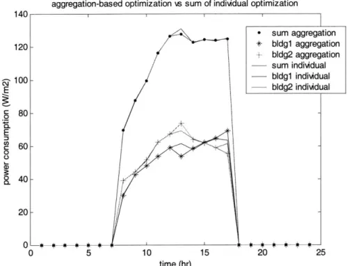
4.2 "Optimal" load aggregation between buildings 1 and 2 112
4.3 "Optimal" load aggregation between buildings 1 and 3 113 4.4 "Optimal" load aggregation between buildings 2 and 3 113
4.5 "Optimal" load aggregation among buildings 1, 2 and 3 114
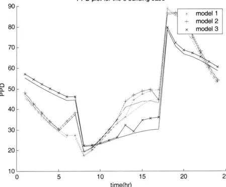
4.6 PPD profiles corresponding to three-building optimal" load aggregation 114
4.7 Comparisons between aggregated and individual load control, buildings 1 and 2 115 4.8 Comparisons between the base case, individual load control, and aggregated 115
load control, buildings 1 and 2
4.9 "Optimal" load aggregation between buildings land 1 116 4.10 "Optimal" load aggregation between buildings 2and 2 116 Page
Figure Figure name and content Page
4.11 "Optimal" load aggregation between buildings 1 and 2, cost-based 117 4.12 "Optimal" load aggregation between buildings 1 and 3, cost-based 118 4.13 "Optimal" load aggregation between buildings 2 and 3, cost-based 119 4.14 "Optimal" load aggregation between buildings 1, 2 and 3, cost-based 120
4.15 Cost comparison for two-building and three-building aggregation 121 4.16 "Optimal" load aggregation between models l and 2 with night cooling 125
available, peak-load based
4.17 PPD plots corresponding to "Optimal" load aggregation between models 1 and 125 2 with night cooling available, peak-load based
4.18 Optimal load aggregation between models 1 and 2 with night cooling available, 126 cost based with $6.5/kW demand charge
4.19 Optimal load aggregation between models 1 and 2 with night cooling available, 126 cost based with varying demand charges below $6.5/kW
4.20 A sequential GA process for a two-building aggregation case 129 4.21 Traces of the Matlab GA process for a two-building aggregation case 131 4.22 Aggregated and individual power profiles for the base and GA optimal cases, 133
two-building fan-based night cooling to minimize the aggregated peak
4.23 Aggregated and individual power profiles for GA and Enumeration optimal 133 cases, two-building fan-based night cooling to minimize the aggregated peak
4.24 Aggregated and individual power profiles for base and the GA optimal cases, 134 two building fan-based night cooling to minimize the total cost
4.25 Aggregated power profiles for the base, GA and Enumeration optimal cases, 134 2bldg fan-based night cooling to minimize the total cost
4.26 "Optimal" load aggregation between buildings 1, 1, and 3 139 4.27 "Optimal" load aggregation between buildings 1, 1, 3, and 3 139
Figure Figure name and content Page
5.2 In-sample residual info: residual plots and ACF plots of residuals 149
5.3 Testing data residuals with the model of Eqn5.4, building type model 1 150
5.4 Relationship between peak load and maximum temperatures in summer, LA 153
5.5 Base load profiles prediction and peak correction 154
5.6 Base load profile prediction vs. simulation 155
5.7 Prediction performance for specific hours over the last 20 days in August 156 5.8 Base load profile prediction improvement based on similar day 157 5.9 Power reduction at hours 11, 12, 13 and 14 vary with base load and thermostat 160
increases
5.10 Power reduction at hour 14 vary with base load and thermostat increase 160 5.11 Power reduction at hours 13-17 vary with thermostat increases 161
5.12 Hourl4 power reduction prediction vs. simulation 161
5.13 PMV increases at hours 12-17 vary with thermostat change 164 5.14 PMV increases at hour 14 vary with base load under different thermostat 164
increases
5.15 Relationship between daytime peak PMV values and peak load in summer, LA 165 5.16 Aggregating two identical buildings with the model-based approach vs. 169
CHAPTER ONE INTRODUCTION
1.1 Background
This thesis work was spurred by the recent energy issues in California, where high peak demand and lack of supply growth created electricity shortages and resulted in high cost and economic inefficiency in 2001. In summer months in California, air conditioning (AC) accounts for 29% of the peak demand with residential AC load contributing 14% and commercial AC load 15% [Ilic 2002]. A variety of solutions have been proposed to reduce the overall electricity consumption and curtail peak demand [Norford 1991, Keeney et al. 1996, Braun et al. 2001]. Our research focuses on the load control by improving the operations in the existing building HVAC (Heating, Ventilating and Air-Conditioning) systems and by aggregating the individual loads based on optimization studies. The optimization problem in this research is multi-objective in the sense that we aim to reduce building electricity consumption while maintaining an acceptable service level - a reasonably comfortable indoor environment.
Electric load aggregation is considered an effective means of maximizing savings and mitigating risks in today's emerging power markets. Load aggregation is the process by which individual energy users band together in an alliance to secure more competitive prices than they might otherwise receive working independently. Aggregation can be accomplished through a simple pooling arrangement or through the formation of clusters where individual contracts are negotiated between the suppliers and each member of the aggregate group. Load aggregation has the following benefits: 1) increased buying power lowers per unit cost for pool members; 2) load diversity among multiple facilities improves load factors, which leads to a smaller demand charge; 3) load aggregation reduces transaction costs and creates economies of scale; 4) a facility may be able to realize significant savings by acquiring a portfolio of energy products that
meets its anticipated needs more efficiently than a full-requirements contract. The candidate buildings do not have to be physically close, and being on the same utility bill with demand charge applied is enough.
A natural question faced by load aggregators is which buildings should go into the aggregation pool. A load aggregator should choose a variety of individual profiles and take advantage of diversification to make aggregation effective. Our research answers this question in a proactive way by allowing load shedding in individual buildings. Based on the improved individual profiles, we explore the cooperation nature between buildings aggregated. By changing building operations temporarily, load shedding offers opportunities to reduce and/or shift peak demand. For example, one building has a much larger peak
demand than another, it might help to curtail the chiller load of the smaller-load building at the time when the larger-load building reaches its peak, so that the coincident peak is reduced. The "cushion" effect of building thermal mass on indoor thermal environment and human beings' adaptability to varying thermal environment allow load to be shifted to a different time without degrading service level.
A building electric load consists mainly of the electricity consumed by lighting, equipment, and HVAC. Cutting equipment electricity use might cause building malfunction and therefore would not be
considered a viable cost-saving approach in this research. Lighting control is straightforward, as the optimal strategy in summer would always be to keep the lowest acceptable lighting level to minimize cooling load. This work focuses on controlling HVAC electricity use. We will explore several major operation changes such as increasing thermostat set points and shutting down chillers temporarily and
will look at the optimal ways of determining these parameters. We choose those control variables that are easy for building operators to change and have good load shedding potential.
1.2 Research overview
In this section we give a brief introduction to what this research intends to accomplish. Related literature will be reviewed in the next section. The entire thesis is to answer one central question - on a short-term basis, e.g. a day or even several hours, how a building operator should control the operations of the target building(s) to minimize energy cost. It could be a building or a group of buildings if aggregation is available. Several key questions are as follows.
e What load control strategies can be implemented?
A variety of load control approaches and their performance are reviewed. Load control scheduling is often a companion problem. Comparison between strategies will be made in Chapters 2-4 with load control implanted to a specific VAV model in this research.
* What optimization algorithms and/or systems are used?
We will review optimization algorithms used in previous building optimization research, their global convergence and computational intensity, ways of handling the multi-objective aspect of the problem, and ease of integration with simulation.
e How are building dynamics represented?
Optimization requires an objective function evaluator - a load model for a building system. It is implemented in two ways in this research: full-scale simulation using EnergyPlus and a simplified load model. A variety of simulation models, including full-scale packages, statistical approximations
and those in between, are reviewed and compared regarding accuracy, computational intensity and ease of integration with optimization.
e How is the aggregation aspect of the multi-building problem captured?
Direct load control research in electrical engineering is reviewed as it deals with a certain type of load control with multiple participants involved. Several optimization schemes are also discussed to handle aggregation.
It is to be noted that most of the examples in this thesis minimize the peak demand. This, as we will argue late in this research, is mathematically equivalent to minimizing the energy cost in terms of
optimization problem structure. Although these two may produce different optimization results, the difference is only a matter of implementation decided by the pricing vector or rate structure used, as the
analysis is identical.
1.3 Literature review
This section reviews previous research addressing the key questions raised in Section 1.2: simulation, optimization, load control strategies and aggregation concerns. We try to address them separately, but most load control research projects cover more than one aspect and therefore only the most important one is emphasized.
1.3.1 Simulation
A big portion of our research relies on building simulation to handle the complex building and plant dynamics. A simulator is essentially a function evaluator in many optimization systems. Three types of simulation are common in research: full-scale simulation package, simplified models, and statistics-based simulation.
a) Full-scale simulator
EnergyPlus, DOE2 and BLAST are examples of full-scale system simulation packages. They cover a wide range of building systems and components, take detailed system description and produce a large number of energy and comfort outputs. Writing modeling script can be quite laborious if started from the beginning, but with knowledge of the software and understanding of the building system, the process does not require sophisticated physics-based modeling skills.
DOE-2 and BLAST are two building energy simulation programs widely used and supported by the US government for more than 20 years. The main difference between the programs is the load calculation method - DOE-2 uses a room weighting factor approach while BLAST uses a heat balance approach. A new energy simulation program, EnergyPlus [Crawley et al. 2001] [EnergyPlus 2003] is built on BLAST and DOE-2 but with a better modular program structure. The major improvement in EnergyPlus over previous energy simulation programs is an integrated (simultaneous loads and systems) simulation for accurate temperature and comfort prediction, rather than taking a sequential approach as in DOE2. In
detail, the process in EnergyPlus is referred to as a Predictor-Corrector process. Loads calculated (by a heat balance engine) at a user-specified time step (15-minute default) are passed to the building systems simulation modules at the same time step. The building systems simulation module, with a variable time step (down to seconds if necessary), calculates heating and cooling system and plant and electrical system response. Feedback from the building systems simulation module to loads not met is reflected in the next time step of the load calculations in adjusted space temperatures and humidity if necessary. As a
comparison, the sequential approach in DOE2 uses a room weighting factor and calculates the zone conditions and determines all heating/cooling loads at all time steps; this information is fed to the air handling simulation to determine system response, and that response does not affect zone conditions; similarly the system information is passed to the plant simulation without feedback. This sequential technique works well when the system response is a well-defined function of the zone temperature. However, in most cases, the system capacity also depends on outside conditions and/or other parameters of the conditioned space. EnergyPlus realizes the fully integrated simulation of loads, systems, and plant through the building systems simulation manager, which makes the simulation modular and extensible.
For the heat and mass balance simulation, the hardwired 'template' systems (VAV, Constant Volume Reheat, etc.) of DOE-2 and BLAST are replaced in EnergyPlus by user-configurable heating and cooling equipment components formerly within the template. This gives users much more flexibility in matching
their simulation to the actual system configurations. EnergyPlus [Crawley et al. 2001] allows users to evaluate realistic system controls, moisture adsorption and desorption in building elements, radiant heating and cooling systems, and interzone air flow - little of which can be simulated well before.
A full-scale simulation package can be plugged in the optimization process, but the full-scale simulator would make the process time-consuming and data processing complex. Such a simulator considers many design and operation aspects, and certain parameters we are particularly interested in are likely be buried in overwhelming details. Although we can post-process the simulation results as we will do late in this
research, this approach provides no direct relation to and insight on how those parameters affect load control.
b) Statistical simulator
Statistical function approximation is a widely-used approach to represent the nonlinear building
dynamics. A variety of artificial neural networks (ANNs) and time series models have been used in load prediction and control research.
0 ANNs
ANNs take advantage of the highly nonlinear properties of their architecture and are able to replicate precisely a variety of dynamics given appropriate training. Large amount of experimental or simulation data are required to train ANNs. Although able to represent complex nonlinearity, ANNs give little insight into the system physics.
[Narendra and Parthasarathy 1990] introduces in detail the concepts of using ANNs to identify and control a dynamic system and demonstrates them using several examples. The paper emphasizes models
for both identification and control. Static and dynamic back-propagation methods for the adjustment of parameters are discussed. Multilayer and recurrent networks are compared and shown to be closely
related, so that they can be studied in a unified fashion. Based on this, the concept of generalized neural networks is presented with four system setups, so that most nonlinear dynamic systems can be generated. Eleven examples based on different plant models are presented to show how the identification and control can be done for nonlinear dynamic systems using neural networks. Of these examples, the identification and/or control results are compared with those of the reference models. The comparison shows that neural networks perform well.
The concept of a general regression neural network (GRNN) is presented in [Specht 1991] as an innovative algorithm of neural network training. GRNN is a memory-based network that provides estimates of continuous variables and converges to the underlying (linear or nonlinear) regression surface. GRNN is a one-pass learning algorithm with a highly parallel structure. Compared to the
back-propagation (BP) algorithm, GRNN is more computationally efficient. In many cases, BP tends to take a large number of iterations to converge to the desired solution. A similar one-pass neural network learning algorithm is the probabilistic neural network (PNN) [Specht 1990]. It is an alternative to BP in
A few tools for system identification and control with neural networks have been developed. If used properly, these tools can potentially make an application problem easier. Some examples of general purpose software that might be applied to system identification and, to a very limited extent, control system design are NeuralWorks Professional II/PLUS from NeuralWare Inc. [Neuralworks 2003], the Neural Network Toolbox for MATLAB from The MatchWorks Inc. [Mathworks 2003], and
NeuroSolutions from NeuroDimension Inc. [Neurosolutions 2003].
In recent years, a wide range of HVAC applications have found neural networks useful. An ANN model [Anstett and Kreider 1993] is used to predict energy use in a complex institutional building without the need for a data acquisition system. The normal predications were done using a formula that was given by a previously developed energy management system using linear regression and other statistical measures. The motivations of incorporating neural networks into the system are 1) to improve the predictive performance; and 2) to provide adaptability to changes in the building's use and energy plant
configuration by taking advantage of the fact that ANN can be developed to update automatically their learned knowledge over time. Ten independent variables are used as inputs, including times, schedule of operations, and air/water temperatures. Four dependent variables, neural network outputs, are usages of
steam, electric, natural gas and water. BP is applied as the training algorithm. Several configurations and different parameters are studied and compared. The results show that ANNs are useful for predicting energy consumption in buildings even with no data acquisition system present.
[Curtis et al. 1993] discusses the results from a computer simulation that used ANNs for predictive control of a hot water coil used to warm an air stream. The coil model itself is a neural network that has been trained on actual data and mimics the nonlinearities of the coil well. Normal PID control of this process has not been very successful, since the controller, feedback, and auxiliary inputs vary across a wide range of values. Based on the system modeled by a well-trained ANN, the predictive control performances are compared between a conventional PID controller and two types of ANN controllers: FANN (future ANN) and IANN (integrated ANN). IANN takes the RMS error over the predicting windows and uses that in the back propagation, but FANN only looks at a single error at some point in the future. The results show that both FANN and IANN have the potential to outperform the standard PID algorithm. Overall, this research shows that neural networks can be used for adaptive and predictive control of a building systems process. The controller is adaptive in the sense that the output of the network used to model the process reflects the changing operating environment, and it is predictive because it examines the future effect of the current controller action.
As an alternative to the BP algorithm and a promising method with computational efficiency and simplicity to implement, GRNN and its applications in HVAC process identification and control have been explored. A local HVAC control example of a heating coil [Ahmed et al. 1996] is chosen to test the
GRNN's effectiveness. A control topology combining feedforward and feedback algorithms is chosen to demonstrate the principle of GRNN and to discuss the role of GRNN in identifying and controlling HVAC control processes. By using this combination topology, the majority of the control signal can be generated from the feedforward block such that the feedback block only deals with a small steady-state error. As a result, the control speed is improved in tracking the set point change. The feedforward component employs a GRNN for HVAC system identification and control, while the feedback component provides a control signal to offset any steady-state error. The GRNN is used to capture the static
characteristics for both valves/dampers and coils. Both simulated and experimental characteristics are used as identification as well test data for the GRNN. The GRNN captures the characteristics well and due to its simplicity exhibits promise for implementation in real controllers. The combined topology algorithm uses GRNN to identify static characteristics and then subsequently uses those in a feedforward controller to generate control signals.
A related research project [Ahmed 1998] compares the combined control topology with the feedback controller for laboratory HVAC applications. The comparison is made for the pressure control sequences commonly found in a laboratory with a VAV system. The control sequence for pressure is developed and a simulation model is built. Simulated results are then presented for the combined, feedforward only, and conventional feedback control approaches. The results indicate that the combined approach performs better than the feedback approach over widely varying operating conditions and different damper characteristics. The combined approach is stable and eliminates all steady-state errors.
To build the load model in our research, ANN could be constructed with previous states, e.g. zone temperature, controls, e.g. chiller status and thermostat set points, and current outdoor temperature and solar radiation as inputs and new states and energy performance as outputs. It can be trained offline by feeding the network simulation or experimental data. A large amount of data will be needed, which is a disadvantage. A neural network model can be hooked up with the optimizer fairly easily. An automatic training process with updated data is desirable.
0 Time series
Gross [1987] gives a thorough and thoughtful review of the short-term load forecasting, which is the prediction of the system load over an interval ranging from one hour to one week. The paper discusses
the nature of the load and the different factors, including economic, time, weather and random effects, influencing its behavior. A detailed classification of the types of load modeling and forecasting techniques is presented. It reviews the peak load models and the load shape models. The latter is categorized into two basic classes: times of day, e.g. spectral decomposition models, and dynamic models, e.g. ARMA and state-space models. Dynamic models represent the stochastically correlated nature of the load process, meaning that the load is not only a function of the time of day, but also of its most recent behavior, as well weather and random inputs. [Papalexopoulos et al. 1990] presented a solid example of a linear regression-based model for short-term load forecasts. Its innovations include
modeling holiday effects using binary variables, modeling temperature using heating and cooling degree functions and robust parameter estimation using weighted least-squares linear regression techniques.
The ASHRAE Application Handbook [1995] reviews some of load forecasting models specifically for buildings. MacArthur et al. [1989] presented a load profile predication algorithm that regresses the
current power consumption to its past values and the time series of exogenous variables such as
temperatures. The algorithm uses a series of recursive least-squares estimators with each having a sample time of one day, so that accurate predications are not limited to one sample time, e.g., an hour, and load profiles for at least a 24-hour period can be obtained. A very simple algorithm for forecasting either cooling or electrical requirements that does not use the 24-hour regressor was presented by Seem et al. [1989] and then further developed and validated by Seem and Braun [1991]. In [Seem and Braun 1991] the average time-of-day and time-of-week trends are modeled using a lookup table with time of day and type of day as the deterministic input variables. Entries in the table are updated using an exponentially weighted moving-average (EWMA) model. Furthermore, the forecasts are corrected through an improved peak load based on a correlation between peak demand and maximum daily temperature forecasts. Residuals are modeled using an auto-regressive moving average (ARMA) model.
Armstrong [2004] develops a transfer function model predicting the conductive cooling load. Together with the time series data of solar radiation, convective heat transfer and outdoor temperatures, and empirical models for chillers, the model relates the detailed dynamic heat transfer process to the plant power consumption.
c) Simplified models
Simplified models fall between full-scale simulation and statistical models. They consist of approximate functional relations for components and systems under study, which makes them more computationally
efficient than full-scale simulation while providing a fair amount of insight into the energy balance and transfer processes.
For chilled water systems that do not have significant thermal storage, a component-based nonlinear algorithm [Braun 1989a] was developed to optimize the system over continuous control variables. This constrained nonlinear procedure was then used as a simulation tool for investigating the optimal system performance. In this nonlinear optimization process, the operating cost and the output of each component in a chilled water system were approximated using a quadratic and linear form respectively. Results of this algorithm led to the development of a simpler system-based methodology for near-optimal control that is simple enough for on-line implementation.
In load control research, the transfer function plays an important role in simplified models. A simulation environment is described in [Braun et al. 2001] in which an inverse modeling approach is taken. The inverse model is based on a transfer function and uses measured data to 'learn' system behavior and provide relatively accurate site-specific performance predictions. Component (fan and chiller) power
models are quadratic functions of flow or temperature variables.
A model used and validated by Morris [1994] is used to enrich a simulation tool [Keeney and Braun 1996] to develop and evaluate control simplifications and strategies. Keeney et al. set up a simulation environment by using the multi-zone building energy analysis subroutine of the dynamic simulation program TRNSYS [Klein et al. 1990] and the empirical functions developed by Braun [Braun 1989.1] for modeling cooling plant power consumption.
An inverse model [Braun 2001] was used to explore the effect of different building thermal mass control strategies on the energy cost. Models are built to represent the behavior of the building, cooling plant, and air distribution system. The transfer functions are used to predict sensible cooling requirements for the building. Empirical or regression results are used for power consumption. Particularly the plant power model is obtained statistically by regressing the power to a polynomial of chilled water
temperature, ambient wet bulb temperature and their squares. Several thermal mass control heuristics with different set point adjustments are compared using this tool.
Armstrong [2004] developed a transfer function based discrete-time, linear and time-invariant system to characterize envelope thermal response, improved the model to preserve its physical feasibility, and estimated the updated model using a nonlinear least squares method. Internal loads are exogenous
variables. The chiller power is characterized by an empirical relation [Ng 1999], and is a function of the cooling load, which bridges the zone temperatures to the power consumption. Certain optimization processes can be applied.
[Wright and Farmani 2001] optimized simultaneously a building's fabric, the size of HVAC system, and the HVAC system supervisor control strategies using a genetic algorithm. A single zone lumped
capacitance model was used to represent the thermal response of the zone, while the HVAC system performance has been simulated using steady component models.
[Constantopoulos et al. 1991] came up with a real-time consumer control scheme for space conditioning under spot electricity pricing. The key assumptions made in building the simulation model are: 1) single conditioned space -neglect circulation effects and assume uniform inside temperature and humidity; 2) lumped model - the shell, the air mass and the other contents of the space have a combined thermal mass; 3) no independent thermal storage is coupled to the main heating or cooling equipment -assume a single piece of equipment; 4) neglect humidity control and focus on temperature control alone; 5) neglect the cycling effect of the thermostat.
d) What simulation approach to use?
The first question is what the precise goals of the simulations. We need a model that has both dynamic building modeling and plant modeling. We need to take into consideration the plant component part-load performance which is important for load control. We need to be able to vary parameters such as
temperature set point, supply air temperature, chilled water temperature, and chiller and fan status on an hourly basis for studying a variety of load control strategies. A full-scale simulation package like EnergyPlus offers all these, and therefore becomes our choice. Later in this research, we have built our own simplified model which preserves several important modeling aspects.
1.3.2 Optimization and load control
As the difference in [Morris et al. 1994] and [Conniff 1991] indicates, whether or not a control strategy is optimized has tremendous impact on the energy performance. This section is categorized by the
optimization methods used in load control and related problems. As a more general field, optimal control is reviewed briefly first. Then attention is turned to the optimal control problems in the building industry and the ways optimization approaches have been applied. A variety of optimization methods have been applied in building control problems and only a few major ones are studied and discussed here: linear and non-linear optimization (LP & NLP), dynamic programming (DP), linear-quadratic optimal control (LQ)
and genetic algorithm (GA). As an indispensable part of optimal control research, different simulation techniques are also reviewed and the integration of simulation and optimization is emphasized. Some references, although not directly related to building industry, are discussed as well because they help understand the methodologies useful to the load control research. Comments are made during the discussion to relate the reference to the load control problem.
a) Optimal Control in general
From the point of view of control theories, optimal control is one particular branch of modem control that sets out to provide analytical designs of a specially appealing type. The system under optimal control not only satisfies the desirable constraints associated with classical control, but it is supposed to be the best possible system of a particular type.
From the point of view of mathematics, optimal control problems are among the most difficult of optimization problems with equality constraints in terms of differential/difference equations and various boundary conditions, while inequality constraints may involve boundary conditions, entire trajectories, and controls [Sage 1977]. The two major theoretical bases in the theory of optimal control are dynamic programming by Bellman and the minimum principle by Pontryagin. The dynamic programming approach is a natural fit for developing the basic relations in the discrete-time optimal control, whereas the minimum principle approach is more suitable for the continuous-time domain. Unfortunately, often times we have to face in complex engineering systems the problem of finding a global optimum for a non-linear optimization problem, which is algorithmically and computationally difficult. In practice,
heuristic-based algorithms, such as genetic algorithm (GA), and direct search methods, such as the Hooke-Jeeves algorithm, are widely used due to their practical efficiency and ease of implement.
From the point of view of research in building industry, the term "optimal control" has been used rather loosely when referring to the control of building operations. Two major methods have been widely used. One is to follow the strict definition of optimal control by proposing optimization algorithms to minimize the cost function. For example, Keeney and Braun [1996] defined the cost as a combination of energy cost and penalized human comfort and minimized it by using the complex method, which is a direct search method that generates a shape in the control variable space that always encloses the minimum point. The other is to conduct extensive simulations with different parameter combinations; the comparison among those simulations indicates the optimal one, which is, to be precise, a suboptimal solution. For example, Henze et al. [1997] developed a simulation environment to investigate a wide
range of key parameters influencing the system's operating cost. The optimal control strategy to minimize the total electricity cost was validated based on the simulation results.
b) Linear and Non-Linear Programming
Two methodologies [Braun 1989a] were presented for determining the optimal control settings for chilled water systems that do not have significant thermal storage. A component-based nonlinear optimization algorithm was developed to optimize the system over continuous control variables. This constrained nonlinear optimization procedure was then used as a simulation tool for investigating the optimal system performance by optimizing over the feasible combinations of discrete controls. In this nonlinear
optimization process, the operating cost and the output of each component in a chilled water system were approximated using a quadratic and linear form respectively. Nonlinear output, linear and nonlinear equality constraints, and inequality constraints were handled using LP or NLP techniques. Results of this
algorithm led to the development of a simpler system-based methodology for near-optimal control that is simple enough for on-line implementation. The system approach involves correlating the overall system power consumption with a single function that allows for rapid determination of optimal control variables and requires measurement of only total power over a range of conditions. The estimating coefficients of this empirical system model involved regression on the results of the component-based optimization algorithm as a simulation tool. The system cost function led to a set of linear control laws for the
continuous control variables. Separate control laws are required for each feasible combination of discrete controls. The number of controls in the system approach is greatly reduced compared to the component approach. With these models, general guidelines for near-optimal performance are developed. Braun's model optimized a snapshot of the plant, and thermal mass played no role in the analysis. Therefore, the results are time-invariant and can be applied to any time spot.
In another closely related work [Braun 1989b], the component-based optimization methodology developed in [Braun 1989a] was utilized as a tool for investigating chilled water systems under optimal control. With this tool, general guidelines for near-optimal performance are developed. These guidelines were incorporated in the system-based near-optimal control methodology, but they are also important to plant engineers for improved control practices. The important uncontrolled variables that affect system performance and optimal control settings are identified. Results and conclusions concerning both control and design under optimal control of chilled water systems are presented.
Braun [1990] studied the dynamic building control, dynamic adjustment of the indoor temperature set points in order to minimize overall operating costs by applying dynamic optimization techniques to
computer simulations of buildings and equipment. He pointed out that the optimization became complicated by the discontinuities associated with the different modes of operations. These modes include mechanical cooling with minimum outside air, mechanical cooling with 100% outside air and free cooling. The approach taken discretized the cost function and applied a non-smooth optimization
algorithm to determine the set of controls that minimize the sum of costs over the specified time.
Determining dynamic optimal cooling control strategies that utilize building thermal mass is formulated as an optimization problem [Keeney and Braun 1996] with zone setting points as controls and a
combination of energy cost and penalized human comfort as the cost. The complex method, an extension of the simplex method to constrained optimization problems, is used to solve this optimization problem over a 24-hour horizon. Based on detailed optimization, two simplified approaches are proposed for
on-line implementations, where one approach takes two constant zone sensible precooling rates and the other applies a constant cooling rate for a given amount of time prior to building occupancy. With much less control variables, these two approaches successfully reduced the computation requirements for
developing optimal strategies. Through the component-model-based simulation, these two approaches were tested with about 1000 different combinations of building, plant and weather. They achieved 95% and 97%, respectively, of the optimal savings relative to conventional control. These simplifications therefore could be used in the development of an on-line controller. In this work, zone set points are the only control, which makes the analysis and optimization easier. In general, developing cooling control strategies which utilize the thermal mass of a building is a formidable optimization problem, especially when on-line implementation is a consideration.
c) Dynamic Programming
Dynamic programming is used [Henze 1997] in determining the optimal control strategies for thermal energy storage systems and a predictive optimal controller for thermal storage systems is developed and
simulated. An optimal storage charging and discharging strategy is planned at every time step over a fixed look-ahead time window utilizing newly available information. The certainty equivalence principle
is used, which fixes the weather and internal gains at their expected values, to make it easier to solve the DP problem. Closed-loop optimization is employed, which means only the first control is executed at
each time step although at each time step the optimization is conducted over the entire planning horizon using appropriate algorithms. The predictive optimal controller is compared to three conventional control heuristics: chiller-priority control, constant-proportion control and storage-priority control. The optimal controller was found to have a significant performance benefit over the conventional controls in the presence of complex rate structures. Compared to the load control problem, the thermal storage control
problem is not very complex in the sense that the system equations and the cost-to-go functions have explicit formulas and fewer controls.
Rossi and Braun [1996] used dynamic programming to obtain optimal service schedules and costs for cleaning the condensers and evaporators of air-conditioning equipment. Cost is defined as a combination of operating cost, human comfort, safety, and environmental criteria. The overall optimization problem is formulated in nested loops using key operating parameters. The innermost loop solves for optimal set of time stages between service tasks using DP. The next loop solves for total number of services in a service cycle using the golden section method by Rao. The outermost loop exhaustively searches for the duration of the service cycle and the time stage of the first service task. In addition, minimum operating costs are compared with regular service intervals (representative of current practice) and a strategy where service is only performed when a constraint is violated (e.g., a comfort reduction). It is found that optimal service scheduling reduced lifetime operating costs by as much as a factor of two over regular service intervals, and by 50% when compared to constrained only service. For practical implementation, a simple near-optimal algorithm for estimating near-optimal service scheduling is developed that does not require on-line forecasting or numerical optimization and is easily implemented within a microcontroller. Over the wide range of cases tested, the near-optimal algorithm gives operating costs that were within 1% of optimal.
A multi-criteria model is described [D'Cruz and Radford 1987] for assisting designers in the choice of form and construction of parallel-piped open plan office buildings at the schematic design stage of building design. The model considers four performance criteria: thermal load, daylight availability, planning efficiency, and capital cost. Pareto-optimal dynamic programming optimization is employed. The model's form and implementation and some typical results are described.
It is worth mentioning that dynamic programming is widely used in the field of operations management (OM). An optimal inventory purchasing policy is determined [Tsitsiklis 1998] with the DP cost-to-go approximated in neuro-dynamic programming (NDP), a method that uses neural nets to approximate the cost-to-go based on the features properly extracted in advance. NDP type of methodologies could possibly be applied in the load control problem. However, the systems in operations management
scenarios are often less complex than most mechanical systems, so problem setup and computation would be more difficult in the load control scenario.
d) Linear-Quadratic Optimal Control
A problem with linear systems and quadratic cost is defined as a linear-quadratic (LQ) problem. The optimal controls can be obtained analytically, which is well known as the Riccati equation [Bertsekas 2000]. Linear and quadratic approximations are valid in many cases in building load research, and LQ is expected to be fairly useful. However, LQ has not been widely used, possibly due to the complexity in the real systems. Hopefully, research that focuses on solving LQ problems using nontraditional and more flexible methods such as neural nets [Lan 1990] and genetic algorithm [Michalewicz 1992] would help improve the situation.
e) Genetic Algorithm
[Wright and Farmani 2001] provided a brief introduction to the major optimization algorithms used in the "whole building optimization" problem. It first described several notable characteristics of the issue: problem variables are a mixture of integer and continuous variables; the problem has non-linear inequality and equality constraints; and the objective functions can be discontinuous. The authors reviewed
previous work and suggested that neither traditional gradient-based methods nor direct search methods are effective for the whole building optimization problem. A genetic algorithm was recommended and used.
A PC-based supervisory controller is developed [Gibson 1997] for a building's energy management and control system to optimize cooling equipment operation. The system provides decision support to determine when to operate central cooling equipment to minimize costs under real-time pricing or conventional time-of-use electric rates. An artificial neural network is used to model the dynamic behaviors of the building and energy equipment while an evolutionary-based search routine, a genetic algorithm is used for optimization. In the GA-based operation schedule planning, Gibson used the bits of the chromosome to represent the status of the cooling equipment in 24 hours. Each chromosome is an operating schedule individual in a "population" of many possible operating schedules. The GA searches for optimal schedule by employing certain techniques of reproduction, crossover and mutation. The ANN-based modeling uses the current external stimuli (outdoor temperature, equipment status, etc.) in conjunction with the previous state of the building to predict the current state of the building. It provides a basic profile of building cooling needs against which each of the individual plans can be evaluated. The
GA initializes and updates the control population. The ANN predicts for each individual its
corresponding load and cost performances and evaluates the fitness which will be sent back to GA. The GA and ANN together form the planning module in this supervisory controller software. A prototype system is installed and operating at a high school in southern California to control a thermal energy
storage system: a conventional screw-type chiller, and a gas-fired, engine-driven chiller. Some lessons were learned during the controller development, and insights were gained in the practical application of both GA and ANN. Examples are how to balance the global optimum and the curse of computation in GA and how to maintain the accuracy of the ANN by applying a neural network monitor, which addresses the relationship between ANN accuracy and the optimization process itself.
Chow [2001] derivd an ANN model of a direct-fired double-effect absorption chiller system. In the paper is discussed the concept of integrating neural network and genetic algorithm in the system optimal control in achieving the final goal of minimizing the operation cost. It is pointed out that to obtain a well
matched but reasonably simple ANN configuration of the system model, a systematic search on the family of architecture is mandatory. Testing should be well monitored and cross-validated. Adequate representation of test data is a prerequisite for a successful outcome.
Wright and Farmani [2001] simultaneously optimized the building's fabric constructions, the size of heating, ventilating and air-conditioning systems, and the HVAC system supervisory control strategy in order to account automatically for the thermal coupling between these building elements. The problem formulation is described in terms of the optimization problem variables, the design constraints, and the design objective functions. The optimization problem is solved using a GA search method. The
conclusion is that the GA is able to find a feasible solution, and it exhibits an exponential convergence on a solution. The solutions obtained are near-optimal, the lack of final convergence being related to variables having a secondary effect on the energy cost objective function. Further research is required to investigate methods for improving the handling of equality constraints and to reduce the number of control variables (which will also improve the robustness of the algorithm).
Wright and Loosemore [2001] investigated the application of a multi-objective genetic algorithm (MOGA) in the search for a non-dominated (Pareto) set of solutions to the building design problems. Compared to the progressive approach that generates the trade-off curve by assigning different weights and repeating the optimization, MOGA employs the Pareto-ranking scheme to form the fitness of each
solution and complete pay-off characteristic in one optimization of the building design. Constraint functions are aggregated by a normalized sum of their violations to form a single design criterion. The results indicate that the MOGA is able to identify the trade-off characteristic between daily energy cost
and zone thermal comfort, and that between capital cost and energy cost. The MOGA exhibits fast progress towards the Pareto optimal solutions.