Channel assignment algorithms and blocking probability analysis for connection-oriented traffic in wireless networks

Channel Assignment Algorithms and Blocking

Probability Analysis for Connection-Oriented

Traffic in Wireless Networks

by

Murtaza Abbasali Zafer

Submitted to the Department of Electrical Engineering and Computer

Science

in partial fulfillment of the requirements for the degree of

Master of Science in Electrical Engineering and Computer Science

at the

MASSACHUSETTS INSTITUTE OF TECHNOLOGY

'August 2003

©

Massachusetts Institute of Technology 2003. All rights reserved.

A uthor ...

...

Department of Electrical Engineering and Computer Science

August 8, 2003

Certified by....

...

Eytan Modiano

ssociate Professor

Thesis Supervisor

Accepted by ... (

Arthur C. Smith

Chairman, Department Committee on Graduate Students

FMASSAHSET

Channel Assignment Algorithms and Blocking Probability

Analysis for Connection-Oriented Traffic in Wireless

Networks

by

Murtaza Abbasali Zafer

Submitted to the Department of Electrical Engineering and Computer Science on August 8, 2003, in partial fulfillment of the

requirements for the degree of

Master of Science in Electrical Engineering and Computer Science

Abstract

We address the problem of dynamic channel assignment and blocking probability for connection-oriented traffic in a multihop wireless network. Specifically, we present an exact blocking probability analysis for a single channel wireless line network and derive blocking probability formulas for both bi-directional and uni-directional calls. In the multiple channel case, we present a simplified analytical model and obtain approxi-mate blocking probability formulas that predict the simulation results very accurately, especially, for low to moderate number of channels. We apply the formulas derived to consider the effect of transmission radius on blocking probability. We show that in a line network with equal length calls, it is preferable to use larger transmission radius; while for a more dense grid network we make simplified analytical arguments show-ing that it is more desirable to use smaller transmission radius. Finally, we present a novel channel assignment algorithm that aims at reducing blocking probability by cleverly reusing the channels while also satisfying the wireless transmission/reception constraints. We compare its performance with other channel assignment algorithms such as the rearrangement, random and the first fit algorithm.

Thesis Supervisor: Eytan Modiano Title: Associate Professor

Acknowledgments

I am profoundly grateful to my advisor, Prof. Eytan Modiano, for his guidance and useful insights on the topic that helped me focus my research in the right direction. I am also thankful to my colleague Anand Srinivas for useful discussions on this topic and other issues in wireless networks.

Finally, I would like to express my gratitude to my parents and family members, especially my brother Ali Zafer, for their continuous moral support throughout my research work.

Contents

1 Introduction

2 Network Model

2.1 Wireless Interference Model . . . . 2.1.1 Uni-directional Calls . . . . 2.1.2 Bi-directional Calls . . . . 2.2 Traffic Model . . . .

3 Line Network

3.1 Introduction . . . . 3.2 Single Channel Wireless Line Network . . 3.2.1 Bi-directional Calls . . . .

3.2.2 Uni-directional Calls . . . .

3.3 Multiple Channels . . . . 3.3.1 Random Channel Allocation Policy 3.4 Summary . . . .

4 Effect of Transmission Radius on Blocking Probability

4.1 Introduction . . . .

4.2 Blocking Probability Analysis in a Generalized Wireless Line Network 4.2.1 Single Channel . . . . 4.2.2 Multiple Channels. . . . . 4.3 Effect of Transmission Radius in a Line Network . . . .

13 17 . . . . 17 . . . . 19 . . . . 20 . . . . 21 23 . . . . 23 . . . . 24 . . . . 25 . . . . 37 . . . . 46 . . . . 47 . . . . 54 55 55 56 57 63 65

4.4 Effect of Transmission Radius in a Grid Network . . . . 4.5 Sum m ary . . . .

5 Dynamic Channel Assignment Algorithms

5.1 Introduction . . . .

5.2 Rearrangement Algorithm . . . .

5.3 Non-rearranging Algorithms . . . .

5.3.1 Random Algorithm . . . .

5.3.2 First Fit Algorithm . . . .

5.3.3 Local Channel Re-use Algorithm (LCRA) 5.4 Simulation Results . . . . 6 Conclusion 76 80 83 83 85 88 91 91 92 94 99

List of Figures

2-1 Interference model for uni-directional data transfer (Z -+ Y in the figure). . . . . 20 2-2 Interference model for bi-directional data transfer (A <-+ B in the

fig-u re). . . . . 21

3-1 A Line Network. . . . . 24

3-2 Constraints on the simultaneous service of adjacent bi-directional calls. 26

3-3 Plot indicating the intersection point between 1/x and 1 + vx2 3 4

3-4 Blocking probability plot for bi-directional calls (plot of PB= 1- 3+2 3

3-5 Plot of g = v'/v for bi-directional calls. . . . . 36 3-6 Constraints on the simultaneous service of adjacent uni-directional calls. 38

3-7 Plot of 9 = v'/v for uni-directional calls. . . . . 46

3-8 Three state Markov process model of the channel on a link. . . . . 49

3-9 State transition diagram for the random channel allocation policy. . . 51 3-10 Comparison of theoretical and simulated values for bi-directional calls

and random channel allocation policy. . . . . 52 3-11 Comparison of theoretical and simulated values for uni-directional calls

and random channel allocation policy. . . . . 53

4-1 Comparison of theoretical and simulated values for r = 2 and r = 10

with 20 channels. . . . . 64 4-2 Comparison of theoretical and simulated values for r = 2 and r = 10

4-3 Blocking probability for calls of length 2 with radius 1 (Eqn. 4.51) and radius 2 (Eqn. 4.52). . . . . 73

4-4 Comparison of blocking probability in a line network for calls of length

3 and 6 and different transmission radius . . . . 76

4-5 Constraints on the service of a bi-directional call in a grid network with nodes having unit transmission radius. . . . . 79

4-6 _{Comparison of blocking probability in a grid network for calls of length}

3 and different transmission radius. . . . . 80 5-1 Multihop channel assignment (S, N1, N2, N3, D is the path of the

mul-tihop call). . . . . 90 5-2 Comparison of blocking probability in a line network for unit length

calls and different channel assignment algorithms. . . . . 95 5-3 Comparison of blocking probability in a grid network for unit length

calls and different channel assignment algorithms. . . . . 96

5-4 Comparison of blocking probability in a line network for 6-hop calls (length 6 units) and different channel assignment algorithms. . . . . . 97 5-5 Comparison of gain in the load for LCRA for 6-hop and 1-hop calls in

List of Tables

3.1 Comparison of theoretically computed and simulated blocking proba-bility values for finite length line network and bi-directional calls. . . 35 3.2 Comparison of theoretically computed and simulated blocking

Chapter 1

Introduction

Wireless communication witnessed a tremendous growth in the last decade and con-tinues to expand rapidly with the development of new technologies. Cellular networks, for wireless voice telephony, have been successfully deployed around the world. How-ever with a rapidly expanding set of wireless users there is a growing need for local wireless networks that can be quickly setup in any terrain. Unfortunately, cellular networks do not provide this flexibility as they require a massive infrastructure in-vestment. Multihop wireless networks are a promising alternative towards achieving this goal.

A multi-hop wireless network (also called an ad-hoc network) is a cooperative

net-work where data streams may be transmitted over multiple wireless links (multiple hops) to reach the destination. The nodes in such a network operate not only as hosts but also as routers forwarding data streams for other nodes that are not within direct transmission range of each other. Unlike its cellular counterpart, this network can be easily deployed in any terrain without the need for any fixed infrastructure. Though easily deployed, a wireless ad-hoc network introduces added complexity into problems of routing [1], scheduling and network connectivity [2]. In addition, such a network should also be able to provide quality of service guarantees to have widespread appli-cation as its cellular counterpart.

Recently, there has been increased focus on issues relating to Quality of Service (QoS) guarantees for wireless ad-hoc networks [3], [4], [5], [6]. The work in QoS guarantees has focussed mainly on finding source-destination routes that satisfy end to end QoS requirements, often given in terms of the required channels (bandwidth). The problem of which channels to allocate from amongst the available channels and the effect of transmission radius on the blocking probability of calls is the focus of this thesis. In this work, we study a line and a grid network as they are good repre-sentatives of a sparse and a dense network respectively.

The problem of dynamic channel assignment has been considered in the context of cellular networks [14], [16], [17], [18]. However, in a multi-hop wireless network the problem differs significantly from its counterpart in the cellular network. In a cellular network (potentially many) nodes communicate only with the nearest base-station. In contrast, in a multi-hop wireless network, transmission of data takes place over multiple wireless links to reach the destination. This imposes additional complexity as non-conflicting channels must be allocated on the wireless links along the source-destination path. Another difference between the two networks is that a cellular network has a regular cell structure which makes the set of interfering cells fixed. While, in a multi-hop wireless network, the set of interfering nodes can be varied by varying the strength of the transmitted signal. This also has the effect of altering the hop length of the calls. With a larger signal strength, a node can communicate with a node further away and reach the destination node in fewer hops albeit at the expense of interference with a larger set of nodes.

The performance metric considered in this thesis is the steady state blocking prob-ability of a call. Blocking probprob-ability as a performance metric has been widely used

by researchers in studying various networks. Some of the work on blocking

proba-bility includes [21], [22] in all-optical networks, [9], [10], [11], [12], in circuit-switched networks and [13], [16], [18], in cellular networks. In [13], Kelly considered a cellu-lar network (where nodes communicate with the nearest base-station) with a linear

topology and compared the fixed and the rearrangement channel assignment algo-rithm. The result was derived in the limit of the length of the line network tending to infinity. We consider a similar limiting argument for the blocking probability analysis of the wireless line network.

The primary contribution of this thesis includes the development of an exact block-ing probability analysis for a sblock-ingle channel wireless line network with sblock-ingle hop calls and a good approximate model for the multiple channel case. We then apply the blocking probability formulas derived to consider the effect of transmission power on blocking probability in a line and a grid network. We show that in a line network it is preferable to use larger transmission radius and communicate directly rather than go multihop to reach the destination (assuming all calls are of the same length); while in a more dense grid network it is more desirable to use smaller transmission radius. Since the line and grid network represent a sparse and a dense network respectively, these results have significant implications in the design of such networks. The result also clearly brings forth the significance of the density of the network on blocking probability in a multi-hop environment. Finally, we develop a channel assignment algorithm for single and multi-hop calls in a wireless network. Our algorithm signifi-cantly outperform the naive random algorithm. More importantly, our results show that the effect of the channel assignment algorithm is more significant when a) the network has a dense topology (e.g., grid) and b) the call length is large. This obser-vation is somewhat intuitive as when the network is dense, efficient packing of the channels becomes critical.

The rest of the thesis is organized as follows. In Chapter 2, we describe the wireless interference and the traffic model. Chapter 3 presents blocking probability analysis for a line network including an exact analysis for the single channel case and an approximation in the multiple channel case. Chapter 4 considers the effect of transmission radius on blocking probability in a line and a grid network. In Chapter 5, we present channel assignment algorithms for multihop calls in a general topology

wireless network and simulation results that compare their performance. Finally, Chapter 6 concludes the work and provides future research directions.

Chapter 2

Network Model

2.1

Wireless Interference Model

A wireless network is modeled as a two-dimensional graph G = (N, A) where N is the

set of nodes and A is the set of wireless links which are assumed to be bi-directional. We say that a wireless link exists between any two nodes if they are within direct transmission range of each other. All nodes in the network have an omnidirectional antenna and are assumed to transmit with the same constant power. We investigate a static wireless network whose topology does not change with time. We refer to the shared resource in the network to service a call as a channel. For example, in a time division multiaccess (TDMA) network, a channel is a time slot within the time-division multiaccess frame and for a frequency time-division multiaccess (FDMA) network a channel is a distinct frequency band. Any transmission or reception is assumed to completely utilize the channel.

To understand the call service mechanism, consider a time division multi-access (TDMA) system. Time is divided into frames which are further sub-divided into slots (called time slots). The total number of time slots in a frame is the total chan-nel resources available in the network. The data transfer between any two adjacent nodes (nodes that are within direct transmission range), takes place in the time slots within a frame. Since we consider only connection-oriented traffic (explained in

Sec-tion 2.2), a time slot must be reserved a priori to allow the data transfer without any interference from the neighboring nodes. Once a time slot is reserved, the call is serviced in that time slot over multiple frames for the entire duration of the call. In case of multi-hop calls, such a mechanism is repeated over all the hops along the entire length of the path. However, neighboring links cannot share the same time slot as interference imposes certain constraints on the simultaneous use of a channel. A frequency division multi-access (FDMA) system is identical to a TDMA system with the time slots being replaced by distinct frequency bands.

We assume a disk model of interference and define the transmission radius of a node (say T) as the radius of a circle (called the transmission circle) outside which the interference due to node T is negligible. Within the transmission radius of node T, we assume complete interference of the signal transmitted by node T with other ongoing transmissions. For any two nodes T and R, we say that node R is a neighbor of node T if R lies within the transmission radius of T. Since the links are assumed to be bi-directional, T is also a neighbor of R. Let the set consisting of neighbors of node

T and node R be denoted as rT and KR respectively. To explain the interference

model, we consider the following example of a data transfer from node T to node R

(T -+ _{R) in channel 7. We refer to node T, as the transmitting node and R, as the}

receiving node. For call T -+ R to be successful, the following criteria needs to be

satisfied.

1. Nodes T and R must not be involved in any other call transmission/reception

in channel -y. This criterion ensures that a node cannot simultaneously serve two calls in the same channel.

2. Neighbors of the transmitting node (P E ArT) must not receive any other data in channel -y. Otherwise the transmission from node T will result in interference and data loss at node P. However, note that a node P E ArT can transmit in

channel -y if this does not violate Condition 3.

in channel y. Otherwise the transmission from node

Q

Q

The above "idealized" model approximates realistic interference assumptions and is commonly used in the study of wireless networks [3], [19], [20]. We consider two types of calls in this work; one involving a uni-directional data transfer and the other a bi-directional data transfer. The next two sections describe each type of call in detail and present examples that illustrate the simultaneous channel use constraints (referred to as the wireless constraints) in either case.

2.1.1

Uni-directional Calls

A uni-directional call from the source node S, to the destination node D, involves

data transfer in one direction from node S to node D (S -> D). Each call is assumed

to require a single channel for service on each hop. For a multihop call, a channel must be reserved on every link along the entire length of the path. The wireless constraints on a single link are explained in the example below (Figure 2-1). Let the path of a multi-hop call be {S, N1, .., Nk, D} where, S is the source node, D is the destination node and N₁, .., Nk are the intermediate nodes. The data transfer takes

place as S -+ N -- N2.. -+ D. Let 71, 72, .. , 7k+1 be the channels selected on the respective links along the path from S to D. The channel assignment is feasible, if for every link i the single hop wireless constraints (Figure 2-1) are satisfied in the chosen channel -yj for that link.

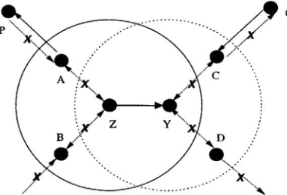
Figure 2-1 example : Consider a single hop data transmission from node Z -+ Y in some channel y. Nodes Z and Y cannot participate in any other transmis-sion/reception in channel y. Nodes A, B are neighbors of Z and they cannot receive any transmission from their neighbors in channel -y. Note that, node A can transmit to node P which is its neighbor but not a neighbor of Z. Neighbors of node

Y are C, D and they cannot transmit in channel -y. Note again that node C can receive from node

Q

C z Y BD

Figure 2-1: Interference model for uni-directional data transfer (Z -> Y in the figure).

2.1.2

Bi-directional Calls

A call between any two nodes S, D is defined as bi-directional if there is data transfer in both directions (S -- D and D -+ S). We continue to make the assumption that

each call requires a single channel for service on every link along the entire length of the path. The actual mechanism by which the data transfer takes place, in either direction on each link, using a single channel is immaterial. One possible way would be to further subdivide the channel reserved on each link. However, we ignore this detail by assuming a bi-directional data transfer on a single "super" channel. The wireless constraints for a single hop bi-directional call are explained in the example below (Figure 2-2). For a multihop call, these constraints must be satisfied at every link on the entire path. Let the path of the multi-hop call be {S, N1, .., Nk, D} along

links S <-> Ni, N <-+ N2,..., Nk <-> D. Let 'Y1,72, .. ,7k+1 be the channels selected on

the respective links along the path from S to D. The channel assignment is feasible, if for every link i the single hop wireless constraints (Figure 2-2), are satisfied in the chosen channel -yj on that link.

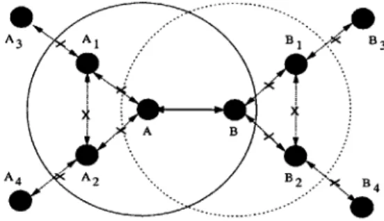
Figure 2-2 example : Consider a single hop bi-directional data transfer between

nodes A and B in channel -y. Since both nodes A and B transmit and receive data (in channel -y) during the duration of the call, all the three conditions as stated ear-lier apply to both the nodes. It follows from Conditions 2 and 3 that neighbors of node A cannot service any other bi-directional call. A similar condition holds for the neighbors of node B. Let a node be labelled inactive (in -y) if it is not involved in transmission on channel y and active (in -y) otherwise. With this notation, we get a more simplified single hop simultaneous channel use constraint as follows. For the bi-directional call A +-+ B to be successful (in channel 'y), neighbors of node A (excluding B) and neighbors of node B (excluding A) must be inactive. As shown in Figure 2-2, nodes A1, A2 are neighbors of A and they cannot service any other call

in channel y (while call A <-+ B is active). Neighbors of node B are B1, B2 and they

cannot service any other call in channel -y. In the figure, the set of interfering data transfers are marked 'X'.

A A B 3B

A B

Figure 2-2: Interference model for bi-directional data transfer (A e B in the figure).

2.2

Traffic Model

All calls in the network are assumed to be connection-oriented. A connection-oriented

call requires dedicated resources for service during the entire duration of the call. These resources are held up while the call is in progress and simultaneously released at the end of the call. We assume that all calls require a single channel for service on each link. The call arrival and departure process is described next. Let Ci, represent

the call arriving at node i and destined for node j. Let Xij(t) denote the arrival process of this call and Zij denote the time this call remains in service. The arrival process Xij(t) is independent of all the other call arrival processes and is assumed to be Poisson with rate A)j. The service time Zij is independent of the arrival times and service periods of other calls and is distributed according to an Exponential distri-bution with mean 1/pij. In this work, we assume a uniform traffic model and set all the arrival rates A)j = A and the service rates pij = M.

We consider bi-directional and uni-directional calls which differ in the set of wire-less constraints on the successful service of a call. To keep the analysis tractable, we consider networks in which calls are either all bi-directional or all uni-directional.

Chapter 3

Line Network

3.1

Introduction

In wireless networks, dynamic channel assignment algorithms can be compared using various performance metrics. As noted earlier, the performance metric in this work is the probability that in steady state an arriving call is blocked. To compute this blocking probability, we construct a stochastic model of the system and analyze its steady state behavior. However, analyzing a general network using the stochastic model is very difficult. Therefore, we consider simpler networks (line network and grid network) with symmetrical loads. These networks help us understand the be-havior of blocking probability under different network parameters and the conclusions drawn here can be applied to more general networks. In this chapter, we analyze a line network where the nodes are located unit distance apart from each other, the transmission radius of each node is unity and all the links have uniform load.

We first consider the simplest non-trivial case of single hop calls and a single chan-nel available in the network. By considering the limiting behavior (length of the line network -+ oc), we obtain an elegant formula that computes the exact blocking prob-ability in the single channel case. We then present a simplified approximate model for computing the blocking probability in the multiple channel case for the random channel allocation policy. This policy is explained in detail in the later sections. The

next chapter builds upon this work and extends it to a more general line network. The insights gained and the formulas derived in this chapter are used in the subse-quent chapter to study the effect of transmission radius on blocking probability in a line and a grid network.

The rest of the chapter is organized as follows. In Section 3.2 we consider a line network with a single channel. We first analyze the blocking probability in a line network with all single hop bi-directional calls (Section 3.2.1) followed by the analysis for single hop uni-directional calls (Section 3.2.2). Section 3.3 presents a simplified model for analyzing blocking probability in the multiple channel case for the random channel assignment policy. Using the simplified model, we derive blocking probability formulas that predict very well the values obtained from simulation results.

3.2

Single Channel Wireless Line Network

Consider a Wireless Line Network with nodes located at positions x = -m, -m+1,. M -1, im. We label these nodes as X-m, _{X-m+i,..., Xm-1, Xm with each node having}

a transmission radius of unity as shown in Figure 3-1. Since the transmission range of every node is unity, each node can communicate directly with a node on its left and a node on its right.

X-m X-m+1 X-m+2 X0 Xm-2 Xm-1 Xm

Figure 3-1: A Line Network.

The reason behind considering a line network with even number of links (2m) is to simplify the blocking probability analysis when we later consider the limiting behavior (with the length of the line tending to infinity). This simplification does not in any way affect the limiting results. The reason for considering an infinite line network is that the edge effects can be eliminated and each node then has an identical

environment. This simplifies the blocking probability analysis and gives elegant and useful results that have applicability for finite length line networks. Before proceed-ing with the analysis, we first present an observation that plays a central role in the subsequent proofs.

Observation: If X and Y are disjoint discrete sets and f(x) and g(y) are any two functions defined on

X

S

f(x)g(y)

(f(x))(

g(y))

(3.1)

(x,y)EXXy xEX yEY

Equation 3.1 can be trivially proved as follows. Let the set X be X1, x2, ..., xk and the

set Y be Y1, Y2, ..., y1 then,

(1 f(x))(1 g(y)) = (f(xi) + ... + f(Xk))(g(y1) + ... + g(yl)) (3.2)

xEX yEY

Expanding the above expression, it can be shown to equal the left hand side of Equa-tion 3.1.

We begin by considering single hop calls and a single channel available in the network. Single hop calls are between nodes that are within direct transmission range of each other. The line network either has all bi-directional calls or all uni-directional calls. In the subsections that follow, we treat each case separately.

3.2.1

Bi-directional Calls

A wireless link (or simply link) is said to exist between any two nodes if they are

within direct transmission range of each other. For a node Xk in the line network, there is a link between nodes (Xk_, Xk) and between nodes (Xk, Xk+1). We label the links in an increasing order with link (X-m, X-m+i) labelled L-m, link (X-m+i,

X-m+2) labelled L-m+i, .., link (Xm-, Xm) labelled Lmi. Thus, there are total 2m

call in service on that link.

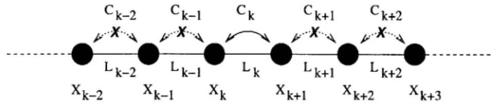
Ck-2 Ck-1 Ck Ck+1 Ck+2

Lk-2 Lk-1 Lk Lk+1 Lk+₂

Xk-2 Xk-1 Xk Xk+1 Xk+2 Xk+3

Figure 3-2: Constraints on the simultaneous service of adjacent bi-directional calls.

Let Ck denote a call between nodes Xk and Xk+1. Ck = 0, if the call is inactive and Ck = 1, if the call is active. Following the constraints as noted in Section 2.1.2, call Ck can be successfully serviced in the single available channel if node Xk-1 (neighbor

of Xk) and node Xk+2 (neighbor of Xk+1) are inactive. This implies that calls k-2,

C-i1, Ck+1, Ck+2 must be inactive (Figure 3-2). We refer to these constraints as the wireless constraints.

" CQ-1 = 0, (Node Xk cannot service any other call). " Ck+1 = 0, (Node Xk+1 cannot service any other call).

" Ck-2 = 0, (Node Xk_1 cannot service any other call as it is within the

trans-mission range of node Xk).

" Ck+2 = 0, (Node Xk+2 cannot service any other call as it is within the

trans-mission range of node Xk+1).

The traffic model follows from Section 2.2. Calls (OQ) arrive according to an inde-pendent Poisson process of rate A. The call holding period of all calls is indeinde-pendent of earlier arrival times and holding periods of other calls and identically distributed according to an Exponential distribution with mean 1/p. There is no admission con-trol and no buffering of calls in the network. If a call cannot be accepted then it is dropped. Otherwise it holds the channel for the entire duration of the call. We refer to this network as WLN-1.

Theorem 1. The blocking probability of a call in a WLN-1 line network with the length of the line network tending to infinity and finite v = A/p is,

x

PB - - 3 (3.3)

1 + 2vx3 where x is the unique root in (0,1] of vx3 + x = 1.

Proof : Let nk(t) be the number of calls Ck in progress at time t. Let v = A/P

and define the vector n(t) = {nk(t)}, k E -M, ..., m - 1. State n is admissible if n > 0 and satisfies the wireless constraints as described earlier. Let g(m) denote the set of all admissible states for a line network with m links (or m + 1 nodes). Since we consider a line network with 2m links, the set of all admissible states is 9(2m). We could express the set g(m) mathematically but the analysis that follows does not require such an explicit description of the state space. The local constraints on the simultaneous use of a channel at a node suffice for the analysis.

The stochastic process (n(t), t > 0) is an aperiodic, irreducible, finite state Markov process and hence has a unique stationary distribution ir(n) = P(n = (nrn, .. , in-i))

given by the following product form solution [7]. The normalization constant in the product form solution is denoted as S(2m), where 2m denotes a line network with 2m links.

1 rn-i~

wr(n) = S(, E g(2m) (3.4)

(2m) r-m nr! nE 2m

The normalization constant S(2m) makes ir(n) a probability distribution and it can be computed by summing ir(n) over all n E 9(2m).

m-1 O

S(2m) =

S

j

nE9(2m) r=-m

Since we are dealing with a single channel network nr = 0 or 1 and nr! = 1. Hence

I m-1 7rS(n) = -() H Vlr 2m) r=-m rn-i S(2m) =

f

Let netta1 = n-m +.. + nm-1, then, 1

- = -r(n) V Vtotal,

Sm(2m)

S(2mn) = E Vntot(m

nEg(2m)

Consider the call {n : n E 9(2m) and

A/BO and let PNB,2m

Then,

Co of the line network. The non-blocking states for call Co are

n-2, n-1, no, n1, n2= 0}, assuming m > 2. Denote this set as

be the probability that in steady state call Co is not blocked.

PNB,2m = ir(n) nEArBo P =

Z

Z

The set of non-blocking states for call Co must have calls C-2, C_1, Co, C1, C2 inac-tive. Therefore, to evaluate the numerator in Equation 3.12 we must characterize the

feasible states of the remaining calls (Cm, .. , C-3 and C₃, .., Cm-i). It turns out that

we do not have to explicitly describe this set. Rather, we can exploit the symmetry in the line network to evaluate the numerator. Before proceeding forward we make the following definitions.

Let gL be the state space of calls -m,., C-3 and G be the state space of calls C3,.., Cm-1. Then, n E g(2m) (3.6) (3.7) (3.8) a E g(2m) _(3.9) (3.10)

9L =_ state space of WLN-1 with m - 2 links

= g(m - 2);

9R astate space of WLN-1 with m - 3 links

= g(m - 3)

Calls C-n, .., C-3 are not affected by the simultaneous service of calls C3, .. , Cm-1

which makes the state space 9L independent of gR. Therefore, the set KBo is the cartesian product of the sets 9L and 9

R _{(by independence) and can be written as,}

ABo = {gLXgR, n-2 n 1, no, n, n2 = 0}. We can now evaluate Expression 3.12

using Equation 3.1. Let, nL = n-m +.. + n-3 and nrR = n3 + .. + nm-1. With this

notation and n- ₂, n-1, no, ni, n2 = 0 we get,

S

Using our notation for the normalization constant we get,

S VL S(m -2) G(m-2) I V" = S(m - 3) 9(m-3)

5

a more simplified way as,

S(m - 2)S(m - 3) (3.17)

NB,2m _S(2m)

The size of the state space, g(m), increases very rapidly with the length of the line. Hence, calculating S(m) by summing over all the feasible states is not practical. However, the symmetry of the line network facilitates an iterative evaluation of S(m). The set of feasible states can be partitioned into a set of states for which the leftmost call is inactive and the set of states for which the leftmost call is active. For the former state space S(m) equals S(m - 1). In the latter state space, the wireless constraint

forces the next two calls on the right (of the leftmost call) to be inactive and the state of the remaining calls on the line is independent of the leftmost active call. Thus, for the latter state space, S(m) equals vS(m - 3). Let SoI{constraint} represent the

evaluation of the function So under the specified constraint.

S(m) = _{S(m)j{leftmost call inactive} + S(m)I{leftmost call active} (3.18)}

S(m) S(m - 1) + vS(m - 3), m > 3 (3.19)

S(k) = 1, k < 0 (defn), S(1) = 1 + v, and S(2) = 1 + 2v.

Using the above equations we can evaluate PNB,2m for a line network with 2m links for any m. Following a similar methodology, we can easily generalize the approach and evaluate the probability of non-blocking PBm of a call Ck, Vk and for any finite

m. It turns out that if we look at the limiting behavior (limm,), an elegant formula

for the blocking probability of any call in the network is obtained. Simulation results (Table 3.1) have shown that this formula very closely approximates the blocking probability for finite length line networks and is much easier to evaluate than the iterative formula presented earlier. The iterative formula becomes cumbersome to deal with as the length of the line increases. We now proceed to consider the limiting behavior. Re-writing Equation 3.17 and taking limits we get,

(S(m-2)S(m-3)) 90 __S(m-1)S(m- 1) PNB,2m S(2m) S(m-1)S(m-1) ) (S(m-2)S(m-3)) lim PB -= m (m-}Sm-) (3.21) M oNB,2m M-.= S(2m) ks(m-1)S(m-1))

To evaluate the denominator in the above equation, we need to evaluate S(2m). This is done by partitioning the state space of WLN-1 into a set of states conditioned on all the possible states of calls (C-1, Co). We then evaluate S(2m) over each of

the partitioned state space and sum them up. There are four cases that need to be considered.

1. C-1, CO both inactive. In this case, calls C-m, .., C-2 do not interfere with calls Ci, .., Cm_1. Thus, the state of calls C-m, ., C-2 is independent of the state of calls C1, .., Cm-1 and we get, (Note that using the earlier notation, feasible state space of {C-m, .. , C-2} = g(m - 1) and the feasible state space of {C1, _.., Cm-1

g(m - 1))

S(2m) =

S

5

9(M-1) gm1

S(2m) = S(m - 1)S(m - 1)

2. C_1 active, Co inactive. Since C_1 is active, calls C-3, C-2, C1 must be inactive. This leaves the state of calls C-m, .. , C_4 independent of the state of the calls

C2,.., Cm-1. The feasible state space of {C-m,.., C 4} = g(m - 3) and the

feasible state space of {C2, .., Cm-1} = g(m - 2).

S(2m) = ( E nf-m+..+n-4) . (

5

g(m-3) g(m-2)

3. C_1 inactive, Co active. By symmetry (with case 2), S(2m) = vS(m - 2)S(m - 3).

4. C-1, Co both active. This state is infeasible.

Thus we have, S(2m) S(2m) = S(2m){C-l1, Co = 0} + S(2m){C_1 = 1,CO = 0} +S(2m){C-1 = 0, CO = 1} = S(m - 1)S(m - 1) + 2vS(m - 2)S(m - 3) (3.22) (3.23)

Plugging Equation 3.23 in Equation 3.21 we get,

S(m-2)S(m-3)

lim PO = urn S(m-1)S(m-1)

m-+oo NB,2m M-oo 1 + 2,S(m-2)S(m-3)

S(m-1)S(m-1)

(3.24)

When m -- oo the probability of non-blocking PNB of any call, by symmetry, is equal to the probability of non-blocking of call Co. We can drop the super script 0 and re-write as (assuming the limit exists which we later show that it does exist),

S(m-2)S(m-3) PNB = liM S(m-1)S(m-1)

m-*o+ 1 + 2,S(m-2)S(m-3)

S(m-1)S(m-1)

(3.25)

To prove the existence of the limit and evaluate its value, we go back and examine Equation 3.19 that evaluates S(m) iteratively.

- S(m - 1) + vS(m - 3) S(m - 1)

S(m)

v

Since the left hand side of the above equation is 1, the limits on the right hand side

S(m) _(3.26)

(3.27) (3.28)

must exist. Let,

n S(m - 1)

M-00 _S(m)

Then,

S(m - 3) S(m - 3) S(m - 2) S(m - 1)

lim =lim .lim lim+C

M-+0 S(m) m-o0 S(m - 2) m-oo S(m - 1) m-o S(m)

Making change of variables, (k = m - 2,1 = m - 1)

S(m - 3) S(k - 1) S(l-1) S(m - 1)

lim =lim lim lim

m-+oo S(m) k--oo S(k)

ILoo

In terms of x, Equation 3.28 can be written as,

1 = x + vX3

(3.29)

We go back and examine what x represents. The normalization constant S(m) is a non-negative monotonically increasing function of m, V v > 0 and gives an indication

of the size of the state space. With this interpretation, x is the state space expansion factor (in terms of the normalization constant S(m)) in the limit (m - oc). For all

finite v > 0, S(k) <; S(k + 1), k > 1 which implies that x E (0, 1]. The existence of a

root of the cubic Equation 3.29 in (0, 1] for any finite v > 0 can be proved as follows.

Re-write Equation 3.29 as,

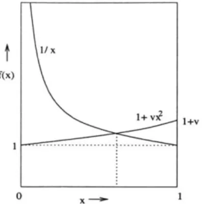
2 1

The function 1/x is a positive decreasing function and takes values between [1, 00) in the interval x E (0, 1]. Function, vX2

+ 1 is a positive non-decreasing function taking

values between (1, 1 + v] in x E (0, 1]. Since we assumed that v > 0, the two curves

t

-b-Figure 3-3: Plot indicating the intersection point between 1/x and 1 + vx2 .

PNB can now be evaluated in terms of x as,

PNB S(m-2)S(m-3) lim -S(m-1)S(m-1) M-00o 1 + 9S(m-2)S(m-3) s(m-1)S(m-1) x3 1+ 2vx3

Finally, the probability of blocking PB = 1 - PNB, is,

PB = 1- ,

1 + 2vx3 Vx3 + x = 1 (3.30)

This completes the proof of Theorem 1.

Z0 0 C '9-'8 '.7 L5 .4 3 2 0 2 3 4 5 6 7 8 9 Load (nlu)

Figure 3-4: Blocking probability plot for bi-directional calls (plot of PB = 1 - X+23-1+v

Figure 3-4 is a plot of PB (Equation 3.30) for various values of the load v. The value of x is computed by finding a root in (0,1] of vX3 + X = 1. Being a cubic

poly-nomial, the root can be evaluated very easily either analytically or using numerical methods.

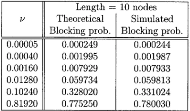
Table 3.1 compares the blocking probability values computed theoretically using Expression 3.30 with the values obtained from simulations of a line network with 10 nodes. In the simulations, blocking probability of the center call is computed as the edge effects are minimal for this call. As seen from the table, the blocking probability formula (Equation 3.30) accurately predicts the values even for small length line networks.

Length = 10 nodes

v Theoretical Simulated Blocking prob. Blocking prob. 0.00005 0.000249 0.000244 0.00040 0.001995 0.001987 0.00160 0.007929 0.007933 0.01280 0.059734 0.059813 0.10240 0.328020 0.331024 0.81920 0.775250 0.780030

Table 3.1: Comparison of theoretically computed and simulated blocking probability values for finite length line network and bi-directional calls.

To understand Equation 3.30 in more detail, we compare it with the standard M/M/1/1 blocking probability expression. The steady state blocking probability in a M/M/1/1 system with load v' is given by,

PB = 1 (3.31)

We make the comparison by calculating an equivalent load v' in the M/M/1/1 block-ing probability expression (Eqn 3.31) that has the same blockblock-ing as that obtained from Equation 3.30 for load v. The significance of the effective load is that, if we isolate a particular link of the line network then load v' on this isolated link would

have the same blocking probability as experienced by the link within the line network (with symmetrical load v). To calculate v', we equate Equation 3.30 and 3.31.

1' 33

= 1- ₁₊₃₃

1 + V' 1 + 2vx3

,1 + (2v - 1)X3

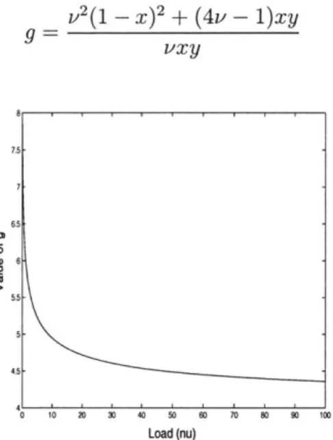
Define factor g as, g = v'/v, then g can be expressed as,

1 + (2v - 1)x3 (3.32)

vx3

A plot of g for different values of load v is presented in Figure 3-5. Evaluating the

limits in Equation 3.32, we get lim_,O g = 5 and limv,o g = 3. The understanding

behind these values of g is that at light load (lim,,o) each arriving call contributes an equivalent load of 5 calls; while at high loads (lim_{1 1} x) each arriving call contributes an equivalent load of 3 calls. These values can be explained in detail as follows.

4.8-4.6 4.4 42 4 3.8 3.6 -3.4 0. 10 20 30 50 0 0 80 90 100 Load (nu)

Figure 3-5: Plot of g = v'/v for bi-directional calls.

v -+ _{0: Each single hop call, Ck, in WLN-1 has four other neighboring interfering}

calls (Ck-2, Ck_1, Ck+1, Ck+2). _{To serve any of these 5 calls, a channel on link Lk}

must be free. In the low load case almost all the calls get served and the chances of more than one call being active from among the 5 calls, C-2, .. , Ck+2, is negligible. Thus, the total rate seen by link Lk is five times the arrival rate and the value of g

as v -+ 0 is 5.

V -+ 00: At very high loads, the highly probable states of the network are the

maximally packed states [15]. In WLN-1 network, the maximally packed states have an active call every two hops apart. The largest set of mutually interfering calls is three and at very high loads (due to maximal packing), these calls mutually block the channels. Thus, the total rate seen by link Lk is three times the arrival rate and the value of g as v -+ 00 is 3.

3.2.2

Uni-directional Calls

We extend the blocking probability analysis of Section 3.2.1 to the case of unidi-rectional calls in a line network. A unidiunidi-rectional call from node Xk to node Xk+1

involves data transfer only in one direction (Xk --+ _{Xk+1). Therefore, in this case,} calls Xk --+ Xk+1 and Xk+1 -+ Xk are distinct. This adds more complexity to the set of interfering calls and manifests itself in a more tedious blocking probability analysis. However, interestingly, an exact expression can be obtained even in this case in the limit of the length of the line network tending to infinity.

The line network is identical to that considered in Section 3.2.1. The wireless in-terference model follows from Section 2.1. The notation for the calls is as follows. We label the call from node X, --+ X1+1 as C21 and the call from node X1+1 - X, as C21+1. Thus, the set of distinct calls in the network are C-2m, C-2m+1, .., 2m-2, C2m-1. Calls

arrive according to independent Poisson processes each of rate A. There is a single channel available in the network. If the arriving call cannot be accommodated for service then it is lost and does not reattempt service request. Otherwise the call is connected and holds the channel for the holding period of the call. The call holding period of all calls is independent of earlier arrival times and holding periods of other calls and Exponentially distributed with mean 1/p.

Consider a particular call Ck _{(k, even). This call is from node} Xk/2 --+ Xk/2+1-The set of local constraints for servicing this call are as follows.

" Since node Xk/2 is only transmitting for the entire duration of call Ck, neighbors

(Xk/2-1 and Xk/2+1) of this node including itself cannot receive any other call.

This implies that calls Ck-4, Ck-2, Ck-1, Ck+1, Ck+3 must be inactive.

" Node Xk/2+1 is the receiver for call Ck. Therefore neighbors (Xk/2 and Xk/₂+2₎

of this node including itself cannot transmit any other call while call Ck is in

progress. This constrains the calls Ck-1, Ck+1, Ck+2, Ck+3, Ck+4 to be inactive.

Combining all the constraints, we find that for call Ck to be successfully serviced

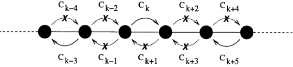
in the available channel, calls Ck-4, CQ-2, Ck-1, Ck+1, Ck+2, Ck+3, Ck+4 must be

inac-tive. Figure 3-6 shows these constraints for call Ck, k being even. Calls marked 'X' must be inactive for call Ck to be successfully serviced . A similar set of conditions

can be obtained for the case when k is odd. We refer to this network as WLN-1(uni).

C k-₄ C k-2 C k C k+2 C k+₄

Ck-3 Ck-l Ck+l Ck+3 Ck+5

Figure 3-6: Constraints on the simultaneous service of adjacent uni-directional calls.

Theorem 2. The blocking probability of a call in a WLN-1(uni) line network with the length of the line network tending to infinity and finite v = A/p is,

xy PB = I - xy(3.33)

v2

(1 - x)2 + 4vxy x and y satisfy the following relations,

x(1- x)2 _+4x 2

= v(1- x)2

2

Y = Vx

Proof: Let nik(t) be the number of calls, Ck, in progress at time t. Let V = A/p

and define the vector n(t) = (nk(t), k E -2m, ..., 2m - 1). State n is admissible if

n > 0 and satisfies the constraints as described earlier. Let H(m) denote the set of all admissible states for a line network with m links (or m + 1 nodes). Since we consider a line network with 2m links (nodes -m, .., m), the set of all admissible states is

N(2m). As in the bidirectional case, an explicit description of the admissible state space is not required. The local constraints on the simultaneous use of a channel suffice for the analysis. The stochastic process (n(t), t > 0) is an aperiodic, recurrent Markov process and hence has a unique product form stationary distribution r(n) = P(n = (n-2m, .. , n2m-1)). The normalization constant in the product form expression

is denoted as N(2m).

1 2m- 1

ir(n) N(2m) _ --- n E l(2m) N(2m -2 r

The normalization constant N(2m) makes ir(n) a probability distribution and it can be computed by summing 7r(n) over all n E h(2m). For a single channel network

nr = 0 or 1 and n.! = 1 and we get,

12m-1 7r(n) = NV2m

J

-H(2m)

S

S

_1

7r(n) )Votal , n E 1-(2m) (3.37)

V(2 m)

N(2m) = vn"'ot (3.38)

nE7H(2m)

states for call CO are {n : n E K(2m), n- 4, n-2, n-1, no, ni, n2, n3, 74 = 0}. Denote

this state space as KBo. _{The probability that call Co is not blocked is,}

PNB =

S

nEgrBo

P B n n B ntotal (3.40)

NnE (2m) Vntotal

To evaluate the numerator in Equation 3.40, we must characterize the set of non-blocking states. It turns out that we do not have to explicitly describe the set KB o.

Rather, as done in the bidirectional case, we can exploit the symmetry in the line network to evaluate the numerator.

Let CL represent the set of calls, C-2m, C-2m+1,.., C-5, C-3 (call C_4 is excluded

as it is inactive in the set KBO) and CR represent the set of calls, C5, C6, .., C2m-1.

The set KBo consists of all the feasible states of calls CL, CR with {C-4, C-2, C-1, CO, C1, C2, C3, C4} = 0. Nodes for the calls CL are not within direct transmission range

of the nodes for CR. Therefore, the calls in CL are not affected by the simultaneous service of calls in CR which makes the state nL = {0-2m, .., n-5, n-3} independent of

the state nR n{75, -., n2m-1} _{and we can apply Equation 3.1. Let,}

nL n-2m + -- + n-5 + n-3

HL feasible state space of calls CL

n = -- +..+ n2m-1

HR afeasible state space of calls CR

We can now evaluate Expression 3.40 using the above notation and Equation 3.1.

5

A/BO HLXHR

1

= (Z vnL)(E vnR)

Z nE(2m) Vntotal

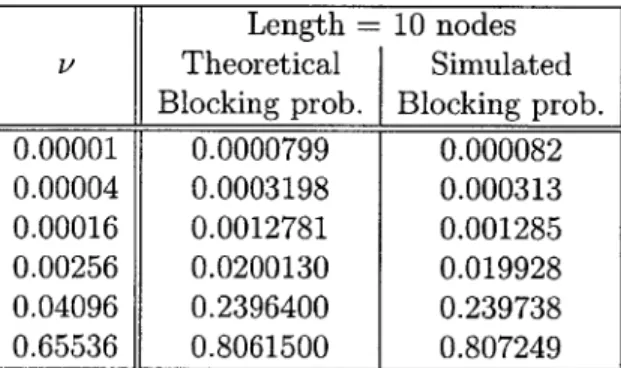
To make the evaluation of the above expression easier, we take the limit, limm--o. The limiting condition eliminates the edge effects of finite length line networks and leads to an elegant formula for the blocking probability of a call. Simulation results (Table 3.2) have shown that this formula very closely approximates the actual blocking probability for finite length line networks. Thus, the result obtained here is not restrictive. When m -- oo the probability of non-blocking, PNB, of any call is by symmetry equal to the probability of non-blocking of call C0O and we can drop the

super script 0. Re-writing Equation 3.43 and taking the limit, limm-,oo, we get,

(

h

n10N lim N(m-1) NB N(m-1)Vnttal(3.44)"

m-+oo m--+oo nEW(2m)

N(m-1)N(m-1)

lim m -- ). ( ( - -1)Vn ) lim m +CO ( NW m -O )

PNB = li1) N(2M) (m-1) (3.45)

im-+0 N(m-1)N(m-1)

To evaluate the limits in the above expression, we use the conditioning argument and the symmetry in the line network as used in the case of bidirectional calls.

V nR = V" {fn5 inactive} + V"R {rn active} HR ?IR,n5=0 HR,n5=1

when n5 = 0 (inactive), the feasible state space of calls {C6, .. , C2m-1} _ 'H(m - 3).

Thus we get,

E VfnR _

5

HR,n5=0 -(m-3)

when n5 = 1, we have n6, n7, n8 = 0 and conditioning on n9 we get,

5

5

Proceeding this way,

V

₊

HR

v nR =N(m

-

+vN(m -

-

Taking the limit (limm-,o) we get,

lim VflR M--0 _{N(m - 1)} N(m - 3) = lim1 m-oo _{N(m - 1)} N(m - 5) m+-vlim +

m-oN(m - 1) v2 m-oo V iN(m - 7)him+ _{N(m - 3)} ... (3.46)

Define the following limits (the existence of these limits is shown later). We choose this definition of the limit as it simplifies the evaluation of the blocking probability expression. lim vN(m) m-oo N(m + 2) lim vN(m) m-+oo N(m + 1) = X y2 = va

In terms of x and y, we can rewrite expression 3.46 as, Z11HR VUnR

lim

M-+0 N(m - 1) - -(X +X2 +X

4_...

v(1 - X)

Following a similar reasoning, we can evaluate limm--o (EHL vnL/N(m - 1)) and the

denominator limm--+o(N(2m)/N(m - 1)N(m - 1)) in Equation 3.45. ZHL V fL lim m-oo N(m - 1) N(m - 2) N(m - 4) = lim + lim v + .. m-oo N(m - 1) m-+oo N(m - 1) - ( + x + 2x3 + ) V v ( - x m odd m even (3.47) (3.48) (3.49) (3.50) (3.51)

To evaluate N(2m), we partition the state space 'H(2m) into a set for which {C-2,

C_1, CO, C1} = 0 (inactive) and a set for which atleast one of the call amongst {C-2,

C_,, Co, C} is active. For the former state space N(2m) = N(m - 1)N(m - 1) and

for the latter state space we make a conditioning argument identical to that made earlier, to obtain the second term in the following equation.

N(2m) = N(m - 1)2 + (3.52) 4v(N(m - 3) + vN(m - 5) + ..)(N(m - 2) + vN(m - 4) + ..) lim

N(2m)

=

+

Using the above results, we can evaluate PB in terms of x and y. However to complete the proof, we need to prove the existence of the limit x and evaluate its value (Note that y can be calculated from x using y2 _{= VX). Using the conditioning}

argument and symmetry of the line network, we evaluate the function N(m + 1) as,

N(m + 1) = N(m) + 2vN(m - 2) + (3.55)

2v2N(m - 4) +.. + 2v1 +1, m even

N(m + 1) = N(m) + 2vN(m - 2) + (3.56)

2vN(m - 4) +.. + 2v , m odd

Dividing by N(m + 1) and taking limit(limm-,o) we get,

1 vN(m) 1 v2_N(m

- 2) ±(.7

1 = -_V lim + - lim + .... (3.57)

m-oO N(m + 1) v m-,o N(m + 1)

Since the left hand side (LHS) of the above equation is 1, the limits on the right hand side (RHS) must exist. This proves the existence of the limits and also provides a way to compute its value. Rewriting Equation 3.57 in terms of x and y we get,