Publisher’s version / Version de l'éditeur:
Vous avez des questions? Nous pouvons vous aider. Pour communiquer directement avec un auteur, consultez la
première page de la revue dans laquelle son article a été publié afin de trouver ses coordonnées. Si vous n’arrivez
Questions? Contact the NRC Publications Archive team at
[email protected]. If you wish to email the authors directly, please see the first page of the publication for their contact information.
https://publications-cnrc.canada.ca/fra/droits
L’accès à ce site Web et l’utilisation de son contenu sont assujettis aux conditions présentées dans le site LISEZ CES CONDITIONS ATTENTIVEMENT AVANT D’UTILISER CE SITE WEB.
Laboratory Memorandum; no. LM-2004-11, 2004
READ THESE TERMS AND CONDITIONS CAREFULLY BEFORE USING THIS WEBSITE. https://nrc-publications.canada.ca/eng/copyright
NRC Publications Archive Record / Notice des Archives des publications du CNRC :
https://nrc-publications.canada.ca/eng/view/object/?id=c9dab33f-7d6b-4cb7-bfa1-9e6e8ae072cc
https://publications-cnrc.canada.ca/fra/voir/objet/?id=c9dab33f-7d6b-4cb7-bfa1-9e6e8ae072cc
NRC Publications Archive
Archives des publications du CNRC
For the publisher’s version, please access the DOI link below./ Pour consulter la version de l’éditeur, utilisez le lien DOI ci-dessous.
https://doi.org/10.4224/8896237
Access and use of this website and the material on it are subject to the Terms and Conditions set forth at
The Dynamic Response of Capacitance Wave Probes
National Research Council Canada Institute for Ocean Technology Conseil national de recherches Canada Institut des technologies oc ´eaniques
Laboratory Memorandum
LM-2004-11
The Dynamic Response of Capacitance Wave Probes
J. Wheeler
April 2004
DOCUMENTATION PAGE
REPORT NUMBER
LM-2004-11
NRC REPORT NUMBER DATE
April 23, 2004
REPORT SECURITY CLASSIFICATIONUnclassified
DISTRIBUTION
Unlimited
TITLETHE DYNAMIC RESPONSE OF CAPACITANCE WAVE PROBES
AUTHOR(S)
Justin Wheeler
CORPORATE AUTHOR(S)/PERFORMING AGENCY(S)
Institute for Ocean Technology, National Research Council, St. John’s, NL
PUBLICATIONSPONSORING AGENCY(S)
IMD PROJECT NUMBER NRC FILE NUMBER
KEY WORDS
Wave probe, capacitance, dynamic, response, static,
calibration
PAGES124
FIGS.16
TABLES2
SUMMARYThis report assesses the dynamic uncertainty in capacitance wave probe measurements
when calibrated and applied statically. It also proves which wave probe circuitry typically
produces the least error over the specified frequency and amplitude ranges.
The experiment was conducted using the Oceanic Corp. 3-Axis Linear Table Arrangement,
which required custom Visual Basic motor controller software and several custom Igor
procedures for run-generation and final data analysis.
Based on the final data analysis, the investigation shows that both the Branckner and
modified wave probe circuitries reported similar dynamic errors (about ± 3 mm) with offsets
close to zero, while the unmodified circuitry consistently showed greater errors with an
offset of 3 mm.
ADDRESS
National Research Council
Institute for Ocean Technology
P. O. Box 12093, Station 'A'
St. John's, Newfoundland, Canada
A1B 3T5
National Research Council Conseil national de recherches Canada Canada Institute for Ocean Institut des technologies Technology océaniques
THE DYNAMIC RESPONSE OF CAPACITANCE WAVE PROBES
LM-2004-11
Justin Wheeler
Th e D yna m ic Re spon se of Ca pa cit a n ce W a ve Pr obe s
Just in Wheeler
LM- 2004- 11
Table of Contents
Table of Figures ... ii
Nomenclature... iii
1. Introduction... 1
2. Three-Axis Linear Table Arrangement... 2
2.1 – Visual Basic Motor Control Software... 3
2.2 – Igor Profile Generation & Analysis Software... 4
2.2.1 – Apparatus Limitations & Acceleration Analysis ... 6
2.2.1.1 – Manual Maximum Acceleration Calculation Methodology ... 7
2.2.1.2 – Methodology of Testing for Maximum Linear Acceleration ... 9
2.2.1.3 – Maximum Acceleration Discussion... 9
3. Data Analysis & Experimental Discussion... 11
3.1 – Igor Data Analysis Software... 11
3.2 – Discussion of Results... 12
4. Conclusions... 20
5. References... 21
Appendix A: Igor Plots of Experimental Data... 22
Appendix B: Motor Controller Source Code ... 40
Th e D yna m ic Re spon se of Ca pa cit a n ce W a ve Pr obe s
Just in Wheeler
LM- 2004- 11
Table of Figures
Figure 1 – 3-Axis Linear Table Arrangement schematic... 2
Figure 2 – Motor control software, main window. ... 4
Figure 3 – Entire movement profile... 6
Table 1 – Experimental failure accelerations of the linear table apparatus. ... 9
Figure 4 – Sample calibration plot for the Branckner wave probe. ... 11
Figure 5 – Nomenclature of zero-crossing analysis parameters. ... 12
Figure 6 – Sample Branckner calibration ... 13
Figure 7 – Sample modified-circuit calibration ... 13
Figure 8 – Sample unmodified-circuit calibration ... 13
Figure 9 – Relative height comparison during vertical movement... 14
Figure 10 - Height difference during vertical movement. ... 14
Figure 11 - Peak difference during vertical movement. ... 15
Figure 12 – Trough difference during vertical movement... 15
Figure 13 – Relative height comparison during circular movement... 16
Figure 14 – Height difference comparison during circular movement... 16
Figure 15 – Peak difference comparison during circular movement. ... 17
Figure 16 – Trough difference comparison during circular movement. ... 17
Th e D yna m ic Re spon se of Ca pa cit a n ce W a ve Pr obe s
Just in Wheeler
LM- 2004- 11
Nomenclature
Sym bol N a m e Un it s
A0 St art Am plit ude m
Af End Am plit ude m
f0 St art Frequency m
ff End Frequency m
p Profile line num ber - -
n Tot al num ber of point s in profile - -
t Current t im e s
∑
T
α Net t orque oz- inα Angular accelerat ion rad/ s2
JT Tot al rot at ional inert ia oz- in- s2
e Ballscrew efficiency [ decim al]
Tm Mot or t orque oz- in
Tg Opposing t or que due t o gr avit y ( for
non-horizont al axes) oz- in
TNL No load t orque oz- in
Tω Viscous t orque oz- in
W Weight lbf
P Ballscrew pit ch rev/ in
Ipk Peak current delivered t o m ot or A Kt Torque const ant of t he specific m ot or oz- in/ A
aL Linear accelerat ion
in/ s2 or m / s2
Jm Rot at ional inert ia of t he m ot or oz- in- s2
Js Rot at ional inert ia of t he ballscrew oz- in- s2
JRL
Reflect ed rot at ional inert ia from t he accelerat ed load as seen by t he
ballscrew
Th e D yna m ic Re spon se of Ca pa cit a n ce W a ve Pr obe s
Just in Wheeler
LM- 2004- 11
1. Introduction
Importance of accurate and reliable wave probes is fundamental to the proper
evaluation of ship hull designs and tank tests where specific types of waves are
generated. Successful experimentation should be both accurate and repeatable, and
knowing the dynamic response of wave probes is useful in evaluating test results. At this
time, it is standard practice to calibrate wave probes using time-independent methods.
One method, for example, is to ‘step’ the probe through a controlled range of wave
heights (or water depths), producing a calibration factor when complete. Assuming that
the same calibration applies to a time-varying set of waves, it is used in experiments.
Purpose of this investigation is two-fold. First, to assess the uncertainty in the
dynamic response of wave probes in general, and second, based on these results, to
choose the best wave probe circuitry to be used in future projects at NRC-IOT.
Currently, there are three wave probe circuits available: Branckner, modified, and
unmodified. The Branckner probe is a commercially available product, while the
modified probe contains updated circuitry of the unmodified wave probe, both of which
were constructed in-house.
To perform this experiment, a three-axis linear table arrangement was used to
move the capacitance wave probe in user-specified paths. In developing profiles for the
probe to follow, several milestones had to be met. First, stable and flexible motor control
software was necessary to control the three-degree-of-freedom arrangement. Second,
software to generate (and evaluate) motion profiles was also required. Apparatus
limitations, mainly maximum motor torque (therefore maximum linear acceleration of the
attached capacitance probe) were calculated and tested empirically to ultimately provide
a safe working range for generated motion profiles. Once the experimentation was
complete, software was also required to automatically analyze, plot, and print data for
final evaluation.
Th e D yna m ic Re spon se of Ca pa cit a n ce W a ve Pr obe s
Just in Wheeler
LM- 2004- 11
2. Three-Axis Linear Table Arrangement
The three-axis linear table arrangement and accompanying mounting frame is an
apparatus designed and owned by Oceanic Corporation and was used to precisely
maneuver the capacitance wave probe.
The apparatus consists of three Parker Daedal ballscrew driven tables, which can
be arranged in several practical ways, allowing the user maximum flexibility in
performable operations. Largest of the three is the x-axis, model 406XR900, which
allows 900 mm of travel. The y- and z-axes are 404XET15 and 404XET07 models,
respectively offering 633 mm and 233 mm of travel. Linear tables are driven by
Aerotech motors, which are powered by Aerotech BA-20 amplifiers. The x-axis utilizes
an Aerotech BM200E brushless DC motor, while the remaining two axes use the smaller
Aerotech BM75E models. Specifications of these components are contained in Appendix
C on their respective manufacturer product sheets. The linear axes would be used to
drive the wave probe in specified patterns, simulating the passing of waves. Yoyo
potentiometers were attached to each axis to record accurate baseline displacements for
comparison with displacements reported by the wave probes. The yoyo potentiometers
have a maximum error of 0.25%.
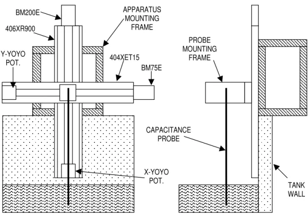
This experiment required only two-degrees of freedom, namely vertical and
horizontal. Since this was the case, the x-axis was mounted vertically and the y-axis was
mounted horizontally onto the x-axis carriage, as shown below in Figure 1.
Figur e 1 – 3- Axis Linear Table Ar r angem ent schem at ic.
APPARATUS
MOUNTING
FRAME
BM200E
406XR900
PROBE
MOUNTING
FRAME
BM75E
404XET15
Y-YOYO
POT.
X-YOYO
POT.
CAPACITANCE
PROBE
TANK
WALL
Th e D yna m ic Re spon se of Ca pa cit a n ce W a ve Pr obe s
Just in Wheeler
LM- 2004- 11
The ‘capacitance probe’ was fixed to a small mounting frame, which was then
attached to the y-axis carriage. The capacitance probe consists of a Teflon-coated
stainless steel cable of 0.44 mm in total diameter. This fine stainless steel wire has a
diameter of 0.36 mm with 0.08 mm of Teflon coating. A capacitance probe works on the
premise that both the wire and the water act as the plates of the capacitor, while the
Teflon coating acts as the dielectric. Thus, as the water level changes, the capacitance
follows accordingly.
A cable is run from the capacitance probe into the wave probe circuitry being
tested. Each of the three wave probe circuits in question convert the capacitance into a
voltage, which is then fed through a signal conditioner panel into the data acquisition
computer. Data is collected at 1000Hz through the GEDAP VMS software package, with
typical run lengths of 780 seconds.
2.1 – Visual Basic Motor Control Software
Once the components were assembled and tested, software was required to control
the movement of the capacitance wave probe. Visual Basic 6 was the language of choice
due to its rapid development rate and wide range of compatibility with various operating
systems. An initial, skeleton package already existed, but for our purposes, a more
full-featured version was required.
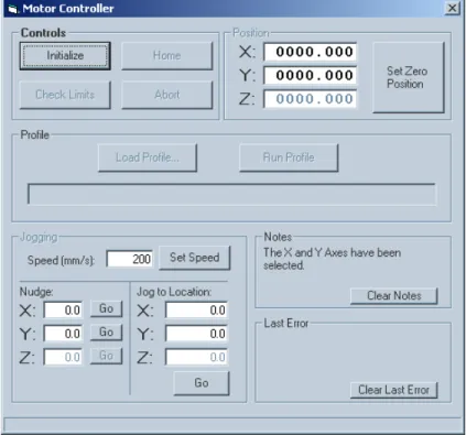
After the software development phase was complete, the motor control program
proved to be very robust and dependable. It has the ability to control each axis
simultaneously and independently and will allow the user to select any arrangement for
axes setup, from the simple single-axis case to the three-axis scenario or any combination
in between. It also provides real-time visual feedback of each carriage position. The user
can choose to move the axes to a position they specify, or can generate a movement
profile in tab-delimited text format and import it into the control program. The profile
defines a time and corresponding x-, y-, and z-axis positions for each ‘point’ in the
movement and the apparatus will respond accordingly. A screen shot of the main
interface of the motor controller software is shown in Figure 2.
Th e D yna m ic Re spon se of Ca pa cit a n ce W a ve Pr obe s
Just in Wheeler
LM- 2004- 11
Figure 2 – Mot or cont rol soft w are, m ain w indow. For source code, see Appendix B.
2.2 – Igor Profile Generation & Analysis Software
Generation of precise and prolonged movement profiles would be very
cumbersome and time consuming to perform manually, even with the use of Microsoft
Excel. A procedure was written in Igor Pro that would perform this task.
It was decided to create sweeped sinusoidal movement profiles for the dynamic
ranges of our test. It is in these sinusoidal regions that the user could examine the
response of the wave probes in time-varying wave scenarios. The Igor procedure
handling this creates the profiles based on the following functions.
)
2
sin(
)
(
t
A
ft
x
=
∆
π
∆
(1)
)
2
2
sin(
)
(
t
=
∆
A
π
∆
ft
+
π
y
(2)
Where
]
/
)
[(
0 0p
A
A
n
A
A
=
+
f−
∆
(3)
]
/
)
[(
0 0p
f
f
n
f
f
=
+
f−
∆
(4)
And
A
0= Start Amplitude [m]
A
f= End Amplitude [m]
f
0= Start Frequency [Hz]
f
f= End Frequency [Hz]
p = Profile line number
n = Total number of points in profile
t = Current time [s]
Th e D yna m ic Re spon se of Ca pa cit a n ce W a ve Pr obe s
Just in Wheeler
LM- 2004- 11
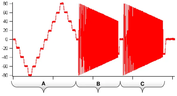
Note that amplitudes and frequencies specified above are user-configurable within
the procedure, allowing for generation of specific movement profiles. During run-time
execution of the function, the user also specifies the total run length (in seconds), from
which Igor determines n, the total number of points in the profile. A complete movement
profile follows in Figure 3, and a zoomed view of the sinusoid is shown in Figure 5.
There were three types of movement profiles generated for the probe to follow.
First, there is a ‘stepped’ range of movement where the probe is moved vertically a given
distance and held there a short period of time. This range was created manually in Excel,
requiring less than twenty entries. It is over this stepped range that static calibrations are
performed, using the x-yoyo potentiometer measurements as the reference data.
Additionally, vertical and circular movements were created. The vertical range
would be used to examine the dynamic response of the wave probes during normal
dynamic calibration. It is known that the small meniscus surrounding the capacitance
probe reduces the accuracy of experiments. In an attempt to remedy this, the circular
movement should produce a much smaller meniscus due to the tangential velocity at the
peaks and troughs. This circular motion represents real tests since water particle velocity
is perpendicular to the probe at the wave peak and trough. Generating these dynamic
ranges required the use of the Igor procedure mentioned above. Vertical movement
utilized only the x-axis while circular movements were slightly more complex. They
were achieved by running both the x- and y-axes simultaneously with matching
frequencies and amplitudes, but with the y-axis
2
π
radians out of phase.
Creation of an entire movement profile, including both static and dynamic ranges
required exporting generated data from Igor into Excel. Within Excel, the user combined
the stepped profile and dynamic ranges of data. Once combined, exporting the profile in
tab-delimited text format was performed from Excel, ready for use by the motor
controller software (see section 2.1). A sample plot of a full run is shown next in Figure
3.
Th e D yna m ic Re spon se of Ca pa cit a n ce W a ve Pr obe s
Just in Wheeler
LM- 2004- 11
A
B C
Figure 3 – Ent ire m ovem ent profile.
Sect ion A show s t he st epped port ion of t he r un, w hile sect ions B and C show dynam ic port ions. Sect ion B consist s of only vert ical m ot ion ( x- ax is) and sect ion C is t he cir cular port ion ( bot h x - and y- axes) .
2.2.1 – Apparatus Limitations & Acceleration Analysis
Apparatus limitations prevented the user from generating motion profiles over the
necessary frequency range (from 0.2 Hz to 1.2 Hz) with large amplitudes. This
frequency range was tested because this is the operating range of the wave-boards in the
Ocean Engineering Basin and the Tow Tank. The largest runs provided by the apparatus
began with an 80 mm amplitude at 0.2 Hz to an end amplitude of 10 mm at 1.2 Hz.
Larger amplitudes might yield a better idea of wave probe response, but the
amplifier-motor-ballscrew arrangements could not physically produce the torque required to move
with higher linear accelerations. Additionally, wave-breaking limits restrict the size of
waves produced at given frequencies, so this 160 mm range was deemed appropriate.
Based on the peak torque provided by the motors, corresponding maximum linear
accelerations were manually calculated. Next, a series of controlled runs were performed
using the apparatus to establish empirical, real-world limitations. Furthermore, the Igor
profile generation software has the ability to analyze the profiles after creation and
automatically plot accelerations. Comparing calculated and empirical maximum
accelerations allowed the user to examine upper-acceleration limits that were shown on
the Igor acceleration plots immediately after profile generation. If accelerations were
shown to reach beyond the upper limits substantially, the apparatus would fail during
profile-execution and the run would have to be re-generated with different amplitude
parameters.
Th e D yna m ic Re spon se of Ca pa cit a n ce W a ve Pr obe s
Just in Wheeler
LM- 2004- 11
2.2.1.1 – Manual Maximum Acceleration Calculation Methodology
Maximum linear accelerations were determined for each of the two axes used in
this set of experiments using the following theory.
Calculations are based on the fact that the sum of torques about the axis of
rotation is equal to the total system rotational inertia multiplied by the angular
acceleration, divided by the efficiency of the system, or
e
J
T
tα
α∑
=
(5)
1Where
= Net torque [oz-in]
∑
T
αα = Angular acceleration [rad/s
2]
J
T= Total rotational inertia [oz-in-s
2]
e = Ballscrew efficiency
Summing the torques about the ballscrew (measured in oz-in),
∑
T
α=
T
m−
T
g−
T
NL−
T
ω(6)
1Where
T
m= Motor torque
T
g= Opposing torque due to gravity (for non-horizontal
axes)
T
NL= No load torque
T
ω= Viscous torque
Additionally,
eP
W
T
g=
2
.
55
(7)
where
T
g= Gravitational torque [oz-in]
W = Weight [lb]
e = Ballscrew efficiency
P = Ballscrew pitch [rev/in]
Also,
t pk mI
K
T
=
(8)
where
T
m= Output motor torque [oz-in]
I
pk= Peak current delivered to motor [A]
K
t= Torque constant of the specific motor [oz-in/A]
Peak current delivered to each motor is dependent upon DIP-switch settings on
the BA-20 amplifier. For the BM200E, the current is limited to 46% of 20 A, which is
9.2 A. The BA-20 amplifier is configured to allow 40% of 20 A to the BM75E y-axis
Th e D yna m ic Re spon se of Ca pa cit a n ce W a ve Pr obe s
Just in Wheeler
LM- 2004- 11
motor, 8 A. The torque constants are found on the spec sheet for the motors. See
Appendix C.
Next,
LPa
π
α
=
2
(9)
where
α = Angular acceleration [rad/s
2]
P = Ballscrew pitch [rev/in]
e = Ballscrew efficiency
a
L= Linear acceleration [in/s
2
]
Substituting (7), (8), and (9) into (6), and solving for the linear acceleration,
P
J
eP
W
T
K
I
e
a
T NL t pk Lπ
2
55
.
2
)
(
⎟
⎠
⎞
⎜
⎝
⎛
−
−
=
(10)
Then, converting linear acceleration from in/s
2to m/s
2is a trivial matter of multiplying
⎥
⎦
⎤
⎢
⎣
⎡
⋅
⎥⎦
⎤
⎢⎣
⎡
⋅
⎥⎦
⎤
⎢⎣
⎡
=
ft
m
in
ft
s
in
a
a
L L2808
.
3
1
12
1
2(11)
Using Equation 11 will yield an acceleration comparable (in units) to that which would
be found through Igor analysis.
To calculate maximum linear acceleration for the vertical x-axis, Equation 10
could be used directly. To find the maximum linear acceleration for the
horizontally-oriented y-axis, Equation 9 must be modified to remove gravitational torque, T
g, term.
For this case,
(
)
P
J
T
K
I
e
a
T NL t pk Lπ
2
)
(
−
=
(12)
and Equation 11 can again be used to convert the units of acceleration.
Several equations use the total rotational inertia, J
Tterm, which consists of, in
this case, inertial effects of the motor, screw, and reflected effect of the load being
accelerated, and has units of oz-in-s
2.
RL s m T
J
J
J
J
=
+
+
(13)
where
J
T= Total rotational inertia
J
m= Rotational inertia of the motor
J
s= Rotational inertia of the ballscrew
And
200105
.
0
P
W
J
RL=
(14)
where
Th e D yna m ic Re spon se of Ca pa cit a n ce W a ve Pr obe s
Just in Wheeler
LM- 2004- 11
J
RL= Reflected rotational inertia from the accelerated load
as seen by the ballscrew
W = Weight [lb]
P = Ballscrew pitch [rev/in]
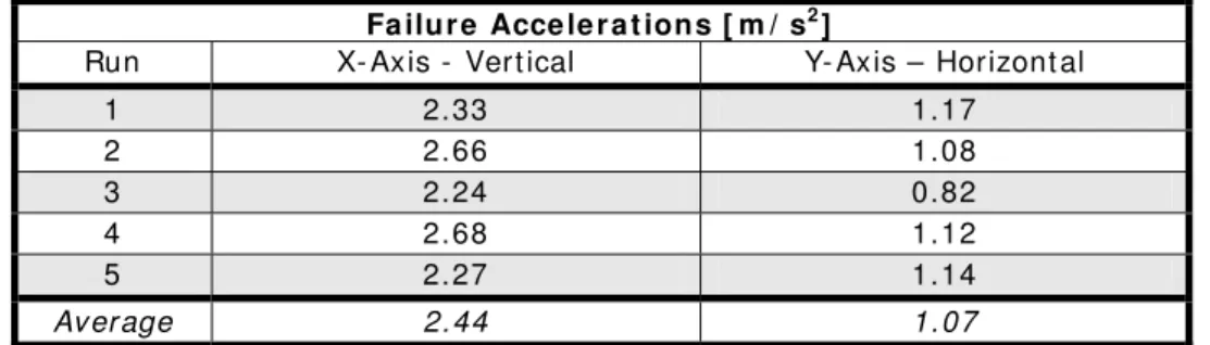
Performing these calculations led to maximum linear accelerations of 1.25 m/s
2for the x-axis and 3.32 m/s
2for the smaller y-axis.
2.2.1.2 – Methodology of Testing for Maximum Linear Acceleration
In an attempt to confirm calculations performed in section 2.2.1.1, a set of runs
was conducted using the linear axes apparatus. These movement profiles were generated
using varying amplitudes, frequencies, and run lengths, attempting to make the setup
produce an amplifier fault.
If a fault was indeed produced, the motor controller software reported the point at
which it occurred in the profile. These failure points were recorded for each run, and
then used to analyze the individual runs in the Igor Profile Generation and Analysis
software. At each point, the software displayed the linear acceleration that caused failure.
A sample of the results is summarized in Table 1.
Fa ilu r e Acce le r a t ion s [ m / s2]
Run X- Axis - Vert ical Y- Axis – Horizont al
1 2.33 1.17 2 2.66 1.08 3 2.24 0.82 4 2.68 1.12 5 2.27 1.14 Average 2.44 1.07
Table 1 – Experim ent al failure accelerat ions of t he linear t able apparat us.
2.2.1.3 – Maximum Acceleration Discussion
A comparison of calculated and actual accelerations shows differences, as one
may expect, between the two for each axis. Although each set does not compare exactly,
they seem to agree within reasonable amounts since most differences can be explained.
Considering values for the vertical x-axis, the calculated value appears to be
lower than that which occurred during experimentation. The calculated acceleration was
about 1.2 m/s
2while experimental values average to about 2.4 m/s
2. One may expect that
calculated values would be more than empirical values, but such is not the case here. It is
possible that although certain losses (for example, small added inertia of the
motor-to-screw coupling) are not taken into account, the motor does output more torque than
calculated. This could be due to several reasons. First of all, one must realize the
difference between maximum and continuous torque (which then translates into
maximum and continuous linear acceleration). Maximum torque is the peak torque that
can be instantaneously produced, while the continuous torque is the highest torque a
Th e D yna m ic Re spon se of Ca pa cit a n ce W a ve Pr obe s
Just in Wheeler
LM- 2004- 11
motor can sustain for longer periods of time. Maximum (or peak) torque is higher than
continuous torque values. It is possible in our case that the maximum calculated
acceleration corresponds closer to a continuous torque value whereas experimental values
show a more instantaneous peak acceleration. Also, the BA-20 amplifier could be
allowing slightly more current to reach the motor than its settings show, resulting in a
higher torque output from the motor. The motor itself may be able to run at
higher-output settings than guaranteed in its specification sheets. It is also possible that the
estimated masses are slightly off and then, going further, one must look at how Igor
calculates derivatives in finding the double-derivative of the movement profile to produce
profile acceleration data. It is possible that small errors created by the Igor differentiation
algorithm result in values that are slightly different than expected.
Results for the horizontally oriented y-axis showed the opposite, but seemingly
more reasonable. The calculated maximum acceleration was about 3.3 m/s
2, compared to
an experimental limitation of about 1.1 m/s
2. In this case, the calculated value seems
much more reasonable since intermittent but excessive vibrations were noticed on this
axis, which certainly caused a large increase in friction, which in turn resulted in a much
lower actual acceleration. Additionally, the added mass effect of the wave probe moving
through the water certainly reduced the obtainable maximum acceleration.
Th e D yna m ic Re spon se of Ca pa cit a n ce W a ve Pr obe s
Just in Wheeler
LM- 2004- 11
3. Data Analysis & Experimental Discussion
3.1 – Igor Data Analysis Software
Analysis of the massive data files collected by the PC was performed by a custom
routine written in Igor on a run-by-run basis. First, the software would perform a
calibration on the data based on the stepped section of the run. Then, the run would be
split into two more sections, the x-range (wherein the probe was moved only vertically),
and the xy-range (wherein the probe was moved in a circular fashion). On each of these
sections, a zero crossing analysis was performed and results plotted. A five-term
polynomial was fitted through each plot to indicate a trend line. Finally, these trend lines
were plotted against each other to graphically indicate the differences in wave-height
measurements between probes.
After importing the DAC file into Igor, the software began data analysis by
calibrating the data reported by the wave probe being tested. This calibration was
performed against the reference x-yoyo potentiometer readings, based on the stepped
range of the movement profile, using a custom least-squares algorithm that is based on
the full-cycle step range. That is, the initial four steps up, eight steps down, then four
steps up to the starting point once again, referring to Figure 3. Calibrations yield a linear
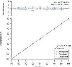
equation and a plot showing residuals and raw data, as seen in Figure 4. These
calibrations were then applied to convert the raw data (in volts) into physical units of
millimeters.
Th e D yna m ic Re spon se of Ca pa cit a n ce W a ve Pr obe s
Just in Wheeler
LM- 2004- 11
Not e t he residuals, equat ion for t he line of best fit and t he R2 value.
Next, the software used this calibrated data in the zero-crossing analysis phase.
Zero-crossing analysis (or ZCA) was performed on both the vertical (x-range) and
circular (xy-range) of each run separately. The idea behind ZCA was, through software,
to count the number of times the data crossed the zero point, recording the time between
crossings, and the maximum (or minimum) data value in each wave cycle. The
maximum value in a cycle was termed a ‘peak’ and the minimum, a ‘trough’. The
difference between a set of peaks and troughs was referred to as a ‘height’, as seen in
Figure 5.
t f ∆ = 1 Height Peak Trough TimeFigure 5 – Nom enclat ure of zero- crossing analysis param et er s.
Analysis software used this data to perform calculations and plot final graphs,
showing trends and probe comparisons. For each probe circuit from each run, four plots
were generated, all against frequency: height difference, peak difference, trough
difference, and relative height. Each respective difference consisted of the probe value
less the baseline yoyo potentiometer value. Relative height consists of the probe value
divided by the yoyo value. Each graph displays the raw data points with a fifth-degree
trend line. These additional plots are included in Appendix A. For a final comparison of
wave probes, trend lines for each probe are compared against each other on summary
plots, which will follow in the next section.
3.2 – Discussion of Results
To assess the uncertainty in the dynamic response of these wave probes, one must
consider both the standard calibration graphs and the final trend line comparison graphs.
There are eight final comparison graphs, shown in the following figures, on which the
experimental discussion is based. Recommendations as to which probe should be used in
future results are also based on these plots.
The static calibration comparisons for each probe show that they are all very
accurate during static tests. Figure 6 shows a Bracnkner calibration, with an R
2= 0.9998.
Th e D yna m ic Re spon se of Ca pa cit a n ce W a ve Pr obe s
Just in Wheeler
LM- 2004- 11
Figure 7 shows that the modified circuitry provides static calibrations with an R
2=
0.9989 while Figure 8 shows the unmodified is also comparable with an R
2= 0.9896.
Both the Branckner and modified circuitries produce very small residuals (up to 2.7 mm)
while the unmodified circuitry reports residuals of nearly 9 mm.
Figure 6 – Sam ple Branckner calibrat ion Figure 7 – Sam ple m odified- circuit calibrat ion
Figure 8 – Sam ple unm odified- circuit calibrat ion
Figures 9 through 16 show the dynamic response of the wave probes when
calibrated under static conditions.
Th e D yna m ic Re spon se of Ca pa cit a n ce W a ve Pr obe s
Just in Wheeler
LM- 2004- 11
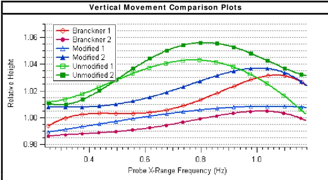
V e r t ica l M ove m e n t Com pa r ison Plot s
Figur e 9 – Relat ive height com parison dur ing vert ical m ov em ent .
Th e D yna m ic Re spon se of Ca pa cit a n ce W a ve Pr obe s
Just in Wheeler
LM- 2004- 11
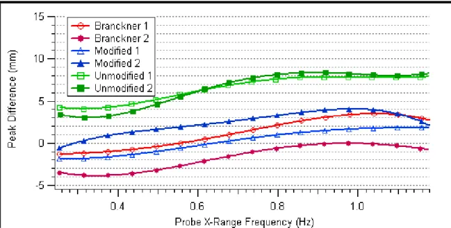
Figure 11 - Peak difference during ver t ical m ovem ent .
Figure 12 – Trough differ ence during vert ical m ovem ent .
In comparing these graphs obtained from the vertical ranges of data, the
Branckner probe tends to report very similar results as the modified probe, while the
unmodified probe not only reports different trends but seems to show a larger biased error
altogether. In terms of height differences (see Figure 10), one could expect the
Branckner circuitry to operate with ±2.5 mm error with a 0.5 mm offset over the
frequency range in question when calibrated statically. The modified probe may produce
errors of ± 2.8 mm with a –0.7 mm offset. Though the unmodified probe circuitry
produces a similar ± 2.5 mm of error, it is centered about a 3.5 mm offset. That is, in
using the unmodified circuitry, the average error might be 3.5 mm as opposed to 0.5 mm
in the Branckner case, or –0.7 mm in the modified case. Similar situations arise in
Th e D yna m ic Re spon se of Ca pa cit a n ce W a ve Pr obe s
Just in Wheeler
LM- 2004- 11
interpreting the peak and trough difference plots (see Figures 11 & 12). The Branckner
and modified probes report similar operating ranges, with average differences less than a
millimeter from zero, while the unmodified probe reports average differences about 3.5
mm above zero.
Interpretation of the circular movement plots may lead to more conclusive results
if similar phenomena occur. See figures 13 to 16.
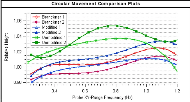
Cir cu la r M ove m e n t Com pa r ison Plot s
Figure 13 – Relat iv e height com parison dur ing circular m ov em ent .
Th e D yna m ic Re spon se of Ca pa cit a n ce W a ve Pr obe s
Just in Wheeler
LM- 2004- 11
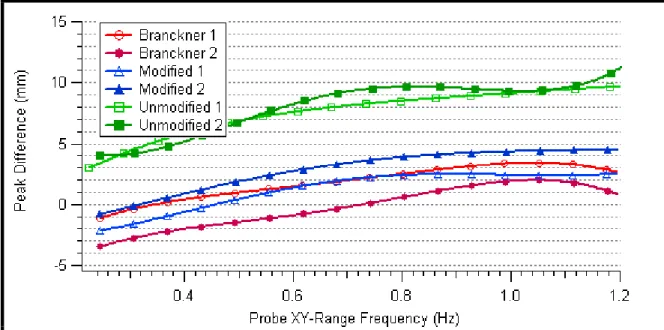
Figure 15 – Peak difference com parison dur ing cir cular m ovem ent .
Figure 16 – Trough differ ence com parison during cir cular m ovem ent .
Figures 13 through 16 show comparable results. The height difference plot
(figure 14) indicates that Branckner and modified probe circuitries operate with an error
of ±2 mm and ±3 mm respectively, with zero offset. The unmodified probe shows an
error of ±3 mm, but again, the average error seems to be about 3 mm. Figure 15, the
peak difference plot shows that the unmodified probe records average differences of
about 6 mm. The trough difference plot in Figure 16 displays a similar result. On these
plots, the Branckner and modified probe data is very close to each other. The peak
difference and trough difference plots from the circular movement (Figures 15 & 16)
show a greater positive bias than those from the vertical movement (Figures 11 & 12).
Th e D yna m ic Re spon se of Ca pa cit a n ce W a ve Pr obe s
Just in Wheeler
LM- 2004- 11
This is most likely due to the stretching of the Teflon-coated wire as the capacitance
probe moves horizontally through the water.
Overall, there appears to be two general patterns in the data. First, both the peak
difference and trough difference seems to increase with frequency. This indicates that
during the movement profile, the wave probes report a mean water level greater than that
before or after the run. This phenomenon is common to capacitance wave probe
measurements and has been referred to as ‘setup’. Another reason for this is that the
water drag produced by pulling the capacitance probe through the water increases
proportionally with frequency, which temporarily stretches the Teflon-coated wire. To
put another way, the positive bias of peak differences and trough differences increases
with cycle frequency. This, however, does not affect the height difference results as the
peaks and troughs increase in the same fashion with time.
Second, as each run progresses, noise or scatter in the recorded data tends to
increase. This could be due to several reasons. The main reason for this is most likely
due to the fact that the capacitance probe is only about 250 mm from the trim tank wall,
which may create interfering reflections of waves in the tank. Another possible reason is
that the water in the tank may contain contaminants, which can build up on the wire
during a run, resulting in slightly more inaccuracies. It may be easier to notice this trend
by looking at the raw data plots found in Appendix A.
Differences between the static calibrations and dynamic records are drawn from
comparisons between the static calibration plots (Figures 6 to 8) and the corresponding
relative height plots shown previously in Figures 10 and 13. The Branckner probe, based
on the static calibration, has residuals ranging from –1.08 mm to 1.04 mm, with an R
2value of 0.9998. Its dynamic response shows maximum height differences of –2 mm to
+3 mm. The modified wave probe shows residuals of –3.15 mm to 2.41 mm with R
2=
0.9987. Dynamic responses show maximum height differences of about –3 mm to +3
mm. The unmodified probe has residuals from –8.93 mm to 6.67 mm (R
2= 0.9896),
while its dynamic records indicate height differences between 0 and 6 mm.
The Branckner and unmodified circuitry show that static calibrations do not
directly explain their response to time-varying water levels. The Branckner electronic
design has a residual range of only about 2 mm while its dynamic counterpart is about 5
mm. The opposite occurs for the unmodified wave probe. Its static calibrations show a
residual range significantly higher than its maximum dynamic height difference range: 14
mm in static residuals compared to only 6 mm for dynamic height differences. It may be
also useful to point out that for the unmodified probe electronics, the average residual
difference tends closer to zero while the average dynamic height difference, as previously
stated, tends to be about 3.5 mm. In contrast, the modified wave probe data has a
residual range of about 5.5 mm while its dynamic range is very much similar. These
discrepancies still indicate that it might be useful to incorporate dynamic responses into
wave probe calibrations. Table 2 summarizes the static and dynamic error comparisons.
Th e D yna m ic Re spon se of Ca pa cit a n ce W a ve Pr obe s
Just in Wheeler
LM- 2004- 11
St a t ic a n d D y n a m ic Er r or Su m m a r ie s [ m m ]
St at ic Dynam ic Height
Difference ( Vert ical)
Dynam ic Height Difference ( Circular) Probe Range Offset Range Offset Range Offset
Branckner ± 1 0 ± 2.5 0.5 ± 2 0
Modified ± 2.75 - 0.7 ± 2.75 0.75 ± 3 0
Unm odified ± 7.80 - 1.1 ± 2.5 3 ± 3 3
Table 2 – St at ic and dynam ic error sum m ar ies.
Based on final data, the most accurate devices are the Branckner probe and the
modified probe. Each of these probes reports very much similar data. If cost were not a
factor, one may choose the Branckner probe since it seems to collect data with less noise
in the channel (see data scatter in Appendix A) than the other probes. If cost is a factor,
the modified probe can most certainly be used with no major tradeoff in accuracy.
Th e D yna m ic Re spon se of Ca pa cit a n ce W a ve Pr obe s
Just in Wheeler
LM- 2004- 11
4. Conclusions
Based on the experimental performance, both goals mentioned in the introduction
are met. First, discrepancies between static calibrations and dynamic responses indicate
that static calibrations do not directly describe dynamic capacitance wave probe
measurements. This may be worth considering during certain types of tank tests since
inherent errors can be expected. Estimates of these errors can be found in Section 3.2,
Table 2.
Finally, experimental data also indicates that the Branckner and modified wave
probes report data with comparable accuracy over the tested frequency range. In static
calibrations, the Branckner probe circuitry reports errors of ± 1 mm, while it reports ± 2
mm with no offset during the circular movements. The modified circuitry reports static
errors of ± 2.75mm with an offset of –0.7 mm, with dynamic height errors ± 3 mm
without an offset. The unmodified probe reports similar error ranges, but it has offsets of
3 mm typically.
So, if cost is no factor, one may choose to purchase and use Branckner wave
probes since they seem less susceptible to noise interference. On the other hand, since
the modified wave probe still produces similar results, it can still be used with
confidence. The unmodified wave probe, in comparison, seems to measure wave heights
with less accuracy. It should not be used for experiments requiring high-accuracy.
Th e D yna m ic Re spon se of Ca pa cit a n ce W a ve Pr obe s
Just in Wheeler
LM- 2004- 11
5. References
1) Aerotech Motion Control Product Guide (1993). Aerotech, Inc., pp.142-143.
2) Ratcliffe, T. and Wilson, M. (1989). “Uncertainty in the Measurement of Ship Model
Wave Profiles and Wave Pattern Resistance”. Proceedings of the 22
ndAmerican Tow
Tank Conference. St. John’s, NF, Canada. August 8 – 11, 1989. pp. 408-416.
Th e D yna m ic Re spon se of Ca pa cit a n ce W a ve Pr obe s
Just in Wheeler
LM- 2004- 11
Th e D yna m ic Re spon se of Ca pa cit a n ce W a ve Pr obe s
Just in Wheeler
LM- 2004- 11
Figure A-1 – Branckner calibration, run 1.
Th e D yna m ic Re spon se of Ca pa cit a n ce W a ve Pr obe s
Just in Wheeler
LM- 2004- 11
Figure A-3 – Modified probe calibration, run 1.
Th e D yna m ic Re spon se of Ca pa cit a n ce W a ve Pr obe s
Just in Wheeler
LM- 2004- 11
Figure A-5 – Unmodified probe calibration, run 1.
Th e D yna m ic Re spon se of Ca pa cit a n ce W a ve Pr obe s
Just in Wheeler
LM- 2004- 11
Th e D yna m ic Re spon se of Ca pa cit a n ce W a ve Pr obe s
Just in Wheeler
LM- 2004- 11
Th e D yna m ic Re spon se of Ca pa cit a n ce W a ve Pr obe s
Just in Wheeler
LM- 2004- 11
Th e D yna m ic Re spon se of Ca pa cit a n ce W a ve Pr obe s
Just in Wheeler
LM- 2004- 11
Th e D yna m ic Re spon se of Ca pa cit a n ce W a ve Pr obe s
Just in Wheeler
LM- 2004- 11
Th e D yna m ic Re spon se of Ca pa cit a n ce W a ve Pr obe s
Just in Wheeler
LM- 2004- 11
Th e D yna m ic Re spon se of Ca pa cit a n ce W a ve Pr obe s
Just in Wheeler
LM- 2004- 11
Th e D yna m ic Re spon se of Ca pa cit a n ce W a ve Pr obe s
Just in Wheeler
LM- 2004- 11
Th e D yna m ic Re spon se of Ca pa cit a n ce W a ve Pr obe s
Just in Wheeler
LM- 2004- 11
Th e D yna m ic Re spon se of Ca pa cit a n ce W a ve Pr obe s
Just in Wheeler
LM- 2004- 11
Th e D yna m ic Re spon se of Ca pa cit a n ce W a ve Pr obe s
Just in Wheeler
LM- 2004- 11
Th e D yna m ic Re spon se of Ca pa cit a n ce W a ve Pr obe s
Just in Wheeler
LM- 2004- 11
Th e D yna m ic Re spon se of Ca pa cit a n ce W a ve Pr obe s
Just in Wheeler
LM- 2004- 11
Th e D yna m ic Re spon se of Ca pa cit a n ce W a ve Pr obe s
Just in Wheeler
LM- 2004- 11
Th e D yna m ic Re spon se of Ca pa cit a n ce W a ve Pr obe s
Just in Wheeler
LM- 2004- 11
Th e D yna m ic Re spon se of Ca pa cit a n ce W a ve Pr obe s
Just in Wheeler
LM- 2004- 11
Form – Form1.frm: This is the main form in operating the motor controller. Option Explicit
'Dim Profile As MovementProfile Private Function CheckLimits() Dim ErrorMessage As String Dim XError As Boolean Dim YError As Boolean Dim ZError As Boolean XError = False
YError = False ZError = False
' Check overall ranges
If (Profile.xMax - Profile.xMin) > (Val(Config("XMax")) - Val(Config("XMin"))) Then
XError = True End If
If (Profile.yMax - Profile.yMin) > (Val(Config("YMax")) - Val(Config("YMin"))) Then
YError = True End If
If (Profile.zMax - Profile.zMin) > (Val(Config("ZMax")) - Val(Config("ZMin"))) Then
ZError = True End If
If XError Or YError Or ZError Then
ErrorMessage = "Profile range too large. (" If XError Then ErrorMessage = ErrorMessage & "X " If YError Then ErrorMessage = ErrorMessage & "Y " If ZError Then ErrorMessage = ErrorMessage & "Z " ErrorMessage = ErrorMessage & "Axis)"
MsgBox ErrorMessage LastError = ErrorMessage CheckLimits = False Exit Function End If ' Check offsets Dim XExceed As Single Dim YExceed As Single Dim ZExceed As Single XExceed = 0
YExceed = 0 ZExceed = 0
If XAxis And Not YAxis And Not ZAxis Then
If (Profile.xMin - XOffset) < Val(Config("XMin")) Then
XExceed = -Round(Val(Config("XMin")) - Profile.xMin + XOffset, 2)
ElseIf (Profile.xMax - XOffset) > Val(Config("XMax")) Then
XExceed = Round((Profile.xMax - XOffset) - Val(Config("XMax")), 2)
End If
ElseIf Not XAxis And YAxis And Not ZAxis Then
Th e D yna m ic Re spon se of Ca pa cit a n ce W a ve Pr obe s
Just in Wheeler
LM- 2004- 11
2)
ElseIf (Profile.yMax - YOffset) > Val(Config("YMax")) Then
YExceed = Round((Profile.yMax - YOffset) - Val(Config("YMax")), 2)
End If
ElseIf Not XAxis And Not YAxis And ZAxis Then
If (Profile.zMin - ZOffset) < Val(Config("ZMin")) Then
ZExceed = -Round(Val(Config("ZMin")) - Profile.zMin + ZOffset, 2)
ElseIf (Profile.zMax - ZOffset) > Val(Config("ZMax")) Then
ZExceed = Round((Profile.zMax - ZOffset) - Val(Config("ZMax")), 2)
End If
ElseIf XAxis And YAxis And Not ZAxis Then
If (Profile.xMin - XOffset) < Val(Config("XMin")) Then
XExceed = -Round(Val(Config("XMin")) - Profile.xMin + XOffset, 2)
ElseIf (Profile.xMax - XOffset) > Val(Config("XMax")) Then
XExceed = Round((Profile.xMax - XOffset) - Val(Config("XMax")), 2)
End If
If (Profile.yMin - YOffset) < Val(Config("YMin")) Then
YExceed = -Round(Val(Config("YMin")) - Profile.yMin + YOffset, 2)
ElseIf (Profile.yMax - YOffset) > Val(Config("YMax")) Then
YExceed = Round((Profile.yMax - YOffset) - Val(Config("YMax")), 2)
End If
ElseIf XAxis And Not YAxis And ZAxis Then
If (Profile.xMin - XOffset) < Val(Config("XMin")) Then
XExceed = -Round(Val(Config("XMin")) - Profile.xMin + XOffset, 2)
ElseIf (Profile.xMax - XOffset) > Val(Config("XMax")) Then
XExceed = Round((Profile.xMax - XOffset) - Val(Config("XMax")), 2)
End If
If (Profile.zMin - ZOffset) < Val(Config("ZMin")) Then
ZExceed = -Round(Val(Config("ZMin")) - Profile.zMin + ZOffset, 2)
ElseIf (Profile.zMax - ZOffset) > Val(Config("ZMax")) Then
ZExceed = Round((Profile.zMax - ZOffset) - Val(Config("ZMax")), 2)
End If
ElseIf XAxis And YAxis And ZAxis Then
If (Profile.xMin - XOffset) < Val(Config("XMin")) Then
XExceed = -Round(Val(Config("XMin")) - Profile.xMin + XOffset, 2)
ElseIf (Profile.xMax - XOffset) > Val(Config("XMax")) Then
XExceed = Round((Profile.xMax - XOffset) - Val(Config("XMax")), 2)
End If
If (Profile.yMin - YOffset) < Val(Config("YMin")) Then
YExceed = -Round(Val(Config("YMin")) - Profile.yMin + YOffset, 2)
ElseIf (Profile.yMax - YOffset) > Val(Config("YMax")) Then
YExceed = Round((Profile.yMax - YOffset) - Val(Config("YMax")), 2)
End If
If (Profile.zMin - ZOffset) < Val(Config("ZMin")) Then
ZExceed = -Round(Val(Config("ZMin")) - Profile.zMin + ZOffset, 2)
Th e D yna m ic Re spon se of Ca pa cit a n ce W a ve Pr obe s
Just in Wheeler
LM- 2004- 11
ElseIf (Profile.zMax - ZOffset) > Val(Config("ZMax")) Then
ZExceed = Round((Profile.zMax - ZOffset) - Val(Config("ZMax")), 2)
End If
ElseIf Not XAxis And YAxis And ZAxis Then
If (Profile.yMin - YOffset) < Val(Config("YMin")) Then
YExceed = -Round(Val(Config("YMin")) - Profile.yMin + YOffset, 2)
ElseIf (Profile.yMax - YOffset) > Val(Config("YMax")) Then
YExceed = Round((Profile.yMax - YOffset) - Val(Config("YMax")), 2)
End If
If (Profile.zMin - ZOffset) < Val(Config("ZMin")) Then
ZExceed = -Round(Val(Config("ZMin")) - Profile.zMin + ZOffset, 2)
ElseIf (Profile.zMax - ZOffset) > Val(Config("ZMax")) Then
ZExceed = Round((Profile.zMax - ZOffset) - Val(Config("ZMax")), 2)
End If Else
LastError = "Error finding exceeding values for selected axes." MsgBox LastError
End If
If (XExceed <> 0) Or (YExceed <> 0) Or (ZExceed <> 0) Then ErrorMessage = "Profile extremes exceed safe limits." If XExceed <> 0 Then
ErrorMessage = ErrorMessage & vbCrLf & "X, by " & XExceed & "mm" End If
If YExceed <> 0 Then
ErrorMessage = ErrorMessage & vbCrLf & "Y, by " & YExceed & "mm" End If
If ZExceed <> 0 Then
ErrorMessage = ErrorMessage & vbCrLf & "Z, by " & ZExceed & "mm" End If MsgBox ErrorMessage LastError = ErrorMessage CheckLimits = False Exit Function End If CheckLimits = True End Function
Private Sub Abort_Click() running = False
WAPIAerAbort End Sub
Private Sub cmdClearNotes_Click() lblSelected = ""
End Sub
Private Sub cmdSetSpeed_Click()
'set the global "velocity" variable based on the numeric value in text box If Not IsNumeric(JogSpeed.text) Then
MsgBox ("Speed must be a numeric value. Setting default value of 200. Press 'Set Speed' to apply the new speed.")
Th e D yna m ic Re spon se of Ca pa cit a n ce W a ve Pr obe s
Just in Wheeler
LM- 2004- 11
JogSpeed.text = "200" Velocity = Val(JogSpeed.text) Else Velocity = Val(JogSpeed.text) End If End SubPrivate Sub Command1_Click() lblLastError.Caption = "" End Sub
Private Sub Execute_Click() 'On Error GoTo done If running Then
MsgBox "Already Running" Exit Sub
Else
If Not CheckLimits() Then Exit Sub End If running = True Jogging.Enabled = False LoadProfile.Enabled = False
sCmd = SeekStart(XAxis, YAxis, ZAxis) SendCommand sCmd
StatusBar.SimpleText = "Located 1st position." ' WaitForMoveToFinish
StatusBar.SimpleText = "Waiting for 5 seconds to continue profile..." sCmd = "DWELL 5000"
SendCommand sCmd 'WaitForMoveToFinish
' Start executing the movement profile.
StatusBar.SimpleText = "Executing loaded profile..."
' Enable Target Tracking mode ' Must do this for each axis
'Call the generic EnableTracking subroutine EnableTracking
'Call generic continue profile subroutine. ContinueProfile
'Call generic disable tracking subroutine once profile is complete. DisableTracking
lblSelected.Caption = "Ready to send abort command..." WAPIAerAbort
lblSelected.Caption = "Abort Command sent." End If
End Sub
Private Sub Form_Load()
If XAxis And Not YAxis And Not ZAxis Then
Th e D yna m ic Re spon se of Ca pa cit a n ce W a ve Pr obe s
Just in Wheeler
LM- 2004- 11
DisableY DisableZ
ElseIf Not XAxis And YAxis And Not ZAxis Then
lblSelected.Caption = "Only the Y-Axis has been selected." DisableX
DisableZ
ElseIf Not XAxis And Not YAxis And ZAxis Then
lblSelected.Caption = "Only the Z-Axis has been selected." DisableX
DisableY
ElseIf XAxis And YAxis And Not ZAxis Then
lblSelected.Caption = "The X and Y Axes have been selected." DisableZ
ElseIf XAxis And Not YAxis And ZAxis Then
lblSelected.Caption = "The X and Z Axes have been selected." DisableY
ElseIf Not XAxis And YAxis And ZAxis Then
lblSelected.Caption = "The Y and Z Axes have been selected." DisableX
Else
lblSelected.Caption = "The X, Y and Z Axes have been selected." End If running = False Velocity = 200 LastError = "" XOffset = 0 YOffset = 0 ZOffset = 0
'Set Profile = New MovementProfile
If Not ParseConfig("C:\u500\mmi\controller.cfg", Config) Then
MsgBox "Error reading configuration file, creating one with default values."
If CreateDefaultConfigFile("C:\u500\mmi\controller.cfg") Then ParseConfig "c:\u500\mmi\controller.cfg", Config
Else
Unload Form1 End If
End If End Sub
Private Sub Form_Unload(Cancel As Integer) If XAxis And Not YAxis And Not ZAxis Then WAPIAerSend "DI X"
ElseIf Not XAxis And YAxis And Not ZAxis Then WAPIAerSend "DI Y"
ElseIf Not XAxis And Not YAxis And ZAxis Then WAPIAerSend "DI Z"
ElseIf XAxis And YAxis And Not ZAxis Then WAPIAerSend "DI X Y"
ElseIf XAxis And Not YAxis And ZAxis Then WAPIAerSend "DI X Z"
ElseIf XAxis And YAxis And ZAxis Then WAPIAerSend "DI X Y Z"
Th e D yna m ic Re spon se of Ca pa cit a n ce W a ve Pr obe s
Just in Wheeler
LM- 2004- 11
WAPIAerSend "DI Y Z" Else
LastError = "Error disabling the axes." MsgBox LastError
End If
WAPIAerClose 0
'now destroy all instances of the forms. Set Form1 = Nothing
Set frmStartup = Nothing Unload Form1
Unload frmStartup End Sub
Private Sub Home_Click()
'Call generic homing subroutine. GoHome
'Set this home position as zero and update the offsets Zero
StatusBar.SimpleText = "Ready..."
End Sub
Private Sub InitializeU500_Click() Dim result As Long
result = Initialize() If result = 0 Then LoadProfile.Enabled = True Abort.Enabled = True Jogging.Enabled = True Position.Enabled = True Timer.Enabled = True Home.Enabled = True StatusBar.SimpleText = "Ready..." Else
LastError = "Error Initializing U500 Controller: " & result MsgBox LastError
End If End Sub
Private Sub JogSpeed_LostFocus()
If Not IsNumeric(JogSpeed.text) Then JogSpeed.text = "200" End Sub
Private Sub JogToLoc_Click() Dim sCmd As String
Dim RealX As Single, RealY As Single, RealZ As Single Dim InRange As Boolean
InRange = True
Th e D yna m ic Re spon se of Ca pa cit a n ce W a ve Pr obe s
Just in Wheeler
LM- 2004- 11
If Not IsNumeric(YJogLoc.text) Then YJogLoc.text = "0.0" If Not IsNumeric(ZJogLoc.text) Then ZJogLoc.text = "0.0"
RealX = XJogLoc.text - XOffset RealY = YJogLoc.text - YOffset RealZ = ZJogLoc.text - ZOffset
If RealX < Val(Config("XMin")) Or RealX > Val(Config("XMax")) Then
MsgBox "X Value out of range. " & Round(Val(Config("XMin")) + XOffset, 2) & " <= x <= " & Round(Val(Config("XMax")) + XOffset, 2)
LastError = "X Value out of range. " InRange = False
ElseIf RealY < Val(Config("YMin")) Or RealY > Val(Config("YMax")) Then MsgBox "Y Value out of range. " & Round(Val(Config("YMin")) + YOffset, 2) & " <= y <= " & Round(Val(Config("YMax")) + YOffset, 2)
LastError = "Y Value out of range. " InRange = False
ElseIf RealZ < Val(Config("ZMin")) Or RealZ > Val(Config("ZMax")) Then MsgBox "Z Value out of range. " & Round(Val(Config("ZMin")) + ZOffset, 2) & " <= z <= " & Round(Val(Config("ZMax")) + ZOffset, 2)
LastError = "Z Value out of range. " InRange = False
End If
If InRange Then
If XAxis And Not YAxis And Not ZAxis Then sCmd = "G0" & _
" X" & Round(RealX * Val(Config("XCal"))) & _ " XF" & Round(Velocity * Val(Config("XCal"))) ElseIf Not XAxis And YAxis And Not ZAxis Then sCmd = "G0" & _
" Y" & Round(RealY * Val(Config("YCal"))) & _ " YF" & Round(Velocity * Val(Config("YCal"))) ElseIf Not XAxis And Not YAxis And ZAxis Then sCmd = "G0" & _
" Z" & Round(RealZ * Val(Config("ZCal"))) & _ " ZF" & Round(Velocity * Val(Config("ZCal"))) ElseIf XAxis And YAxis And Not ZAxis Then
sCmd = "G0" & _
" X" & Round(RealX * Val(Config("XCal"))) & _ " XF" & Round(Velocity * Val(Config("XCal"))) & _ " Y" & Round(RealY * Val(Config("YCal"))) & _ " YF" & Round(Velocity * Val(Config("YCal"))) ElseIf XAxis And YAxis And ZAxis Then
sCmd = "G0" & _
" X" & Round(RealX * Val(Config("XCal"))) & _ " XF" & Round(Velocity * Val(Config("XCal"))) & _ " Y" & Round(RealY * Val(Config("YCal"))) & _ " YF" & Round(Velocity * Val(Config("YCal"))) & _ " Z" & Round(RealZ * Val(Config("ZCal"))) & _ " ZF" & Round(Velocity * Val(Config("ZCal"))) ElseIf XAxis And Not YAxis And ZAxis Then
sCmd = "G0" & _
" X" & Round(RealX * Val(Config("XCal"))) & _ " XF" & Round(Velocity * Val(Config("XCal"))) & _ " Z" & Round(RealZ * Val(Config("ZCal"))) & _ " ZF" & Round(Velocity * Val(Config("ZCal"))) ElseIf Not XAxis And YAxis And ZAxis Then
sCmd = "G0" & _
" Y" & Round(RealY * Val(Config("YCal"))) & _ " YF" & Round(Velocity * Val(Config("YCal"))) & _ " Z" & Round(RealZ * Val(Config("ZCal"))) & _