Benchtop testing of polyethylene passive sampling towards a quantitative analysis of volatile organic compounds (VOCs) in soil vapours

Benchtop Testing of Polyethylene Passive Sampling Towards a Quantitative

Analysis of Volatile Organic Compounds (VOCs) in Soil Vapours

by

Yu Xiang Jaren Soo

BSc Chemistry

Imperial College London, 2014

ARCHVES

OF rECHNOLOLGY

JUL 02 2015

LIBRARIES

SUBMITTED TO THE DEPARTMENT OF CIVIL AND ENVIRONMENTAL

ENGINEERING IN PARTIAL FULFILLMENT OF THE REQUIREMENTS FOR THE

DEGREE OF

MASTER OF ENGINEERING IN CIVIL AND ENVIRONMENTAL ENGINEERING

AT THE

MASSACHUSETTS INSTITUTE OF TECHNOLOGY

JUNE 2015

C 2015 Yu Xiang Jaren Soo. All rights reserved.

The author hereby grants to MIT permission to reproduce and to

distribute publicly paper and electronic copies of this thesis document

in whole or in part in any medium now known or hereafter created.

Signature of author:

Signature redacted

Depar

ent of Civi nd Environmental Engineering

8 May 2015

Certified by:

Signature redacted

Philip M. Gschwend

Pord Professor of Civil and E

ironment Engineering

Th is Supervisor

Accepted by:

Signature redacted

Heidi M. Nepf

Donald and Martha Harleman Professor

Chair, Departmental Committee for Graduate Students

Benchtop Testing of Polyethylene Passive Sampling Towards a Quantitative

Analysis of Volatile Organic Compounds (VOCs) in Soil Vapours

by

Yu Xiang Jaren Soo

Submitted to the Department of Civil and Environmental Engineering on May 8, 2015 in Partial fulfillment of the

requirements for the Degree of Master of Engineering in Civil and Environmental Engineering

Abstract

The feasibility of polyethylene (PE) as a passive sampler for quantitative analysis of volatile organic compounds (VOCs) was analysed in this work by means of a benchtop testing. A benchtop physical model was setup, which consisted of a jar of glass beads or sand, containing a known mass of toluene as the compound of concern (COC). A beaker of water was placed in the physical model as a second form of measurement of toluene concentration in the air. The concentration of toluene in the air of the physical model was measured using the PE passive sampler and compared to results found by measurement toluene in water in the beaker. The PE-inferred vapour concentrations were consistent with the measurements in the water. With benzene, toluene, ethylbenzene and o-xylene (BTEX) selected to be quantified in the actual soil, both the PE passive sampler and the water-based measurement showed inconsistency in contrast to previous experiments with glass beads and sand. This inconsistency could probably be due to the presence of biodegradation. Nonetheless, if proved consistent in future, PE passive sampling can also be used to estimate the concentrations of compounds based on molecular weight in absence of known literature values of required parameters.

Thesis Supervisor: Philip M. Gschwend

Acknowledgements

I would like to express my gratitude to my group members, David Jensen and Hanqing Liu

for the opportunity to work with them and also helping me in various aspects of the project as an when. Thank you so much!

To the two most important people that made this project possible, Prof Phil Gschwend and John MacFarlane, thank you. Thank you John for all the assistance provide to me during the course of this project. I really appreciate the time and patience you have in helping me getting things done. And also to Phil, I really appreciate the patience you have in guiding us throughout the course of this research and also for being very accepting for all the work I've produced.

Also to the batch of 2015 MEng Civil and Environmental Engineers, thanks for just being there to just talk and share some of your thoughts, frustrations, everything! Will certainly miss being in the MEng room.

To my friends around me or in any parts of the world, thanks for the company throughout this 9 months. It was certainly a joy knowing that there are people standing by even from afar, they certainly made a difference to me.

And most importantly, to my family members, for their continuous support and care toward me not just through this Masters, but the 4 years spent overseas. Thanks for enduring all my frustrations and also for being there during times of joy. Now I am finally done!

Table of Contents

Abstract...

2

Acknowledgem ents...

3

Abbreviation ...

6

Chapter 1: Introduction...

8

1.1 Chem ical contaminants in the environm ent...

8

1.2 Repercussions of chemical contaminants in the environment ...

9

1.3 Current limitations in environmental risk assessm ent...

10

1.4 Soil gas measurement techniques ...

11

1.5 Quantitative passive sampling as a method to improve measurement accuracy

...

12

1.6 Aim and objective of this project ...

14

Chapter 2: Approaching the problem ...

16

2.1 Sm all-scale testing a necessity...

16

2.2 Benchtop testing as a means of controlling variability...

17

2.3 Benchtop testing in this experim ent ...

17

2.3.1 Conditions and parameters known ... 18

2.3.2 Setup of the experiment ... 19

2.3.3 W ater in beaker as a second form of measurement...21

2.4 Aim s and objective of this experim ent ...

22

Chapter 3: Experim ental details...

23

3.1 Apparatus and chemical handling...

23

3.2 Properties and the treatment of PE ...

23

3.3 Properties and treatment of media ...

23

3.4 Instrum entation specifications and methods ...

24

3.4.1 Gas chromatography... 24

3.4.2 Gas chromatography with purge and trap ... 25

3.4.3 Gas Chromatography - Mass Spectrometry... 25

3.5 Measurem ent of porosity ...

26

3.6 Generic passive sampling experim ental methods ...

27

3.6.1 Experiment with glass beads ... 27

3.6.2 Experiment with sand ... 28

3.7 W ater extraction of COC from PE ...

28

3.8 Preparation of standards ...

29

3.9 Precision of results...

30

Chapter 4: Results and Discussion...

32

4.1 Experim ental jar with glass beads ...

32

4.2 Experim ental jar with sand ...

33

4.3 Investigation on actual soil...

34

4.3.1 Identification of compounds... 35

4.3.2 Quantitative analysis of contaminants in soil... 36

Chapter 5: conclusion and future w ork ...

39

5.1 Conclusion ...

39

5.2 Future w ork ...

39

5.2.1 Pentane extraction instead of w ater extraction of chem icals... 39

5.2.2 Perform ance reference com pounds (PRCs) ... 40

5.2.3 M easurem ent of biodegradation and field testing... 41

References ... 42

Abbreviation

Biochemical Oxygen Demand

Benzene, Toluene, Ethylbenzene, Xylenes Compound(s) of concern

Electron lonisation

Environment Protection Agency Flame lonisation Detector Gas Chromatography

Gas Chromatography - Mass Spectrometry Minimum detection limit

Polyethylene

Polycyclic aromatic hydrocarbon Performance Reference Compound Semipermeable membrane devices Underground Storage Tanks Volatile Organic Compounds

Chapter 1

:

Introduction

This chapter had been jointly written along with Hanqing Liu and David G. Jensen, both of whom were working on separate aspects of the project. Liu focused on obtaining physical properties of VOCs with regards to transport in, out and within the polyethylene (PE).1 Jensen focused on developing the mass transfer model for soil gas and also developing the probe prototype to be used for the eventual field testing.2

1.1 Chemical contaminants in the environment

The potential for chemical contaminant release to the environment is ubiquitous in the modern world. For example, in 1986 the United States started a programme dedicated to the regulation of underground storage tanks (USTs). As of September 2014 there were over

570,000 active USTs, most of which contain petroleum products for service stations. These

USTs cannot be designed to last forever and thus each of them will leak overtime. In fact since 2009, the Environment Protection Agency (EPA) has consistently reported between

6000 and 7000 confirmed releases of contaminants by registered USTs every year.3 These

USTs are spread throughout the US. Just the state of Massachusetts contains approximately

10,000 active USTs, which is equivalent to almost 1 potential release site every square mile.

USTs are an example of one way that a single type of contaminant can be released. Chemical contaminants exist in many modern day products and manufacturing process and thus accidental spills and leaks will be expected. Though contaminants are certainly entering the environment more slowly with improved regulation, the only way to completely stop their releases is to stop using them altogether. Since this is not likely to occur in the near term, it is important to be prepared to evaluate the impact of leaks and spills as they occur.

1.2 Repercussions of chemical contaminants in the environment

Though the discharge of contaminants to the environment is inevitable, not all of these discharges necessarily present an unacceptable risk to humans and the environment. The EPA describes three pieces of information that are needed in order to conduct a risk

assessment at a contaminated site: inherent toxicity of the chemical, how much exposure a receptor has with the contaminated medium, and how much of the chemical is present in an environmental medium (soil, water, air).4 It is the method of determining this final piece of information that is of particular interest for the purpose of this project, specifically with regards to vapour intrusion.

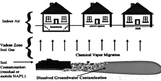
Vapour intrusion is an important exposure pathway in risk assessment. When a contaminant, such as petroleum, is leaked into the ground, gravity pulls it down through the soil until it hits the water table or impermeable soil layer. Certain low molecular weight chemicals, commonly referred to as volatile organic compounds (VOCs), are constantly volatilising from the petroleum pure phase or from groundwater containing these dissolve contaminants. Vapour intrusion is how these VOCs are transported from the contaminated source to indoor air where they can be inhaled (Figure 1.1).5 Most vapour intrusions do not result in high concentration of contaminants in indoor air. However, because humans spend a significant portion of their day inside buildings6 and breathe a large volume of air, inhaling relatively low concentrations of these hazardous chemicals can result in unacceptable levels of risk leading to potential chronic health problems.

Indoor Air=n

eaft z

I I

I I

Vdlos Zoos

cbub.i VOW MIgrW Soil

M1

Figure 1.1: A conceptual model of potential vapour intrusion pathways

1.3 Current limitations in environmental risk assessment

Screening algorithms are one way to predict indoor air concentrations of VOCs. These models help determine if a contaminated site will pose significant health risks and they can also guide remediation decisions. One of the most important and useful inputs to a vapour intrusion screening model is reliable soil gas concentrations of contaminants. Vapour concentration measurements are necessary because mass transport in soil is largely influenced by molecular diffusion from high concentration to low. Furthermore additional measurements can help to confirm model accuracy.

Unfortunately there appears to be a problem with current modelling and measurement methods. In a comparison of seven commonly used vapour intrusion algorithms, Provoost

et al. showed that most predicted soil gas concentrations overestimated the observed

values.6 The deviation tended to be less than an order of magnitude, but was sometimes as much as four orders of magnitude greater (Figure 1.2).6 This deviation is not surprising as the individual complexities of each site make predicting soil gas concentrations imperfect.

However the discrepancy in soil gas concentration draws into question, not only to our understanding of the soil environment for modelling, but also the accuracy of current soil gas measurement techniques.

1.E+08

o JEM o VLH A VOLaSOil -CS04 0 Risc x DF SE DF NR

1.E+0 - -- - - ---

---1.E+07 --- ---

---i.E+0

1 .E0 ---. .- 1 --- 1E

0.+06

--0? 0,

F ,gure -. : --- t --- 14 d- -bs-rve ---d-td -----sco c ntat

1.E+04 h

X X

1.E+03 --- -

Q---i.+ OI I a I1

11E-02 11-01 i.1+00 i.E+01 1.E+02 11E+03 11E+04 11E+05 Observations (MgWM3)

Figure 1.2: Scatter plot of observed and predicted soil gas concentration from several sites using 7 different vapour intrusion models6

1.4 Soil gas measurement techniques

Original attempts to determine soil gas concentrations used extrapolations from bulk soil sampling. This technique can be helpful to delineate contaminated soil, but it has been shown to underestimate actual vapour concentrations.7 Another problem with the technique is significant loss of VOCs during the sampling process.7 Because of these challenges, a push was made for technology that could directly sample and analyse soil gas for contaminants. Currently the most common method is active gas sampling, which involves the insertion of a hollow probe into the soil. Soil gas can then be drawn into a container that is sent to the lab for analysis. This has the advantage of allowing direct soil

gas analysis and it can be done relatively quickly (10-30 samples/day).7 There are however some disadvantages. Active soil gas sampling requires the removal of a large quantity of soil vapour in order to purge the system. The removal of a large volume of soil gas means it may be sampling air from an unknown distance away from the probe. The forceful removal of soil vapour also has the potential to disturb equilibrium conditions yielding unrepresentative results.7

An alternative method involves the use of passive samplers. This method takes an absorptive material and places it in the soil for several days to a week. During this time the VOCs in the soil gas partition into the absorptive material. The sampler itself is then sent to a lab where contaminants are extracted and analysed. The concentrations in the soil vapour cannot be reported, but masses reported for multiple sampling locations, collected after the same deployment time, can create a map of relative magnitudes. This map can then be used to help identify "hot spots" on the surface. This method has distinct advantages because it does not forcefully remove soil gas, it works well in a wide range of soil types for a wide range of VOCs, and it can reduce sampling costs.8 Furthermore it has been argued that the accuracy of passive sampling is greater than that of active because there are fewer sources of error (mechanical and human) and because the sampler equilibrates with the background concentration, it can reduce temporal deviations.9 1 0 The notable problems are

that it has a long sampling time and it does not provide quantitative results.7

1.5 Quantitative passive sampling as a method to improve measurement accuracy

A new passive sampling method suggested by Fernandez et al. for sediments uses

performance reference compounds (PRCs) impregnated in polyethylene (PE) before deployment to allow calculation of contaminant concentrations in porewater of

sediments.1' In the simplest form of the method, added PRCs have similar chemical and physical properties to the target chemical, usually a deuterated or 13C-labelled species. In this way, the effective diffusion of the PRC out of the PE should match the diffusion of the target compound into the sampler. After deployment, a measurement of the remaining PRC mass permits the calculation of the extent to equilibrium reached. Using this information and the deployment time, one can then back calculate the concentration of the target compound in the environment.

Using a PRC for every target compound, however, will become expensive so Fernandez et al. proposed using a method to extrapolate PRC properties to different compounds." Using a

1D diffusion mass transport model they were able to generate a linear regression from a

small number of PRCs with which to infer necessary mass transfer properties for all other target compounds.

In a later study of quantitative passive sampling in sediments, Apell and Gschwend validated the PRC equivalent diffusion assumption.12 They showed that they could accurately determine equilibrium concentrations in sediment porewater using PE removed at several different times prior to equilibrium (Figure 1.4). Furthermore they confirmed the ability to use a linear regression generated from the mass transfer model to infer chemical transport properties. Using these inferred properties they were able to calculate PE-deduced concentrations that were not significantly different than equilibrated results found independently.

- g...- - a-- - - U 1 Deduced Luilibrium Concentration C0 0 0 i Target Accumu 0.1 U PRC Loss 0.0 001 1

Time Measured Porewater (ng/L)

Figure 1.3: Left image shows cartoon of target chemical and PRC concentration in sediments over time and

deduced equilibrium concentrations (black squares) compared to measured equilibrium values. Equilibrium

concentrations were obtained using the mass transfer model developed by Fernandez et al.11 and input into a

GUI interface developed by Tcaciuc et aL13 Right image shows comparison of measured and PE-deduced

porewater concentrations for 3 PCB congeners in 7 different sediments. Solid line represents the 1:1 relationship between the axes and the dotted line shows a root-mean-squared error (0.232) in the logarithmic

plot. 12

1.6 Aim and objective of this project

Quantitative passive sampling retains the benefits of previous non-quantitative passive sampling techniques, while in addition providing accurate concentration measurements. The goal of this project is to test whether quantitative passive sampling will be successful in accurately measuring contaminant concentrations in soil gas.

However in order to develop a new method which can be widely adopted in future, it needs to have several features for which people can be drawn to it. One possible feature is being able to meet minimum detection levels (MDL) required by the regulators (EPA) for a wide variety of compounds. If detection limits of this sampling method does not reach that of minimum detection levels dictated by regulators, they are unable to determine if the site they test on would be able to meet safety standards. In addition, this method of sampling should provide a low cost alternative to current technology so that people are willing to adopt this method of sampling. These features are non-exhaustive, because any

improvements on current technology made, while retaining benefits of these current ones, will be able to draw people's attention to this new method.

In the development of the quantitative passive sampler for soil, a mass transfer model was first developed. This was done by adjusting the mass transfer model for sediments to include a vapour phase. However to be able to use the model, accurate measurements of chemical and physical properties for target VOCs must be obtained. Specifically experimental values of PE-water and PE-air partitioning coefficients and PE diffusion coefficients must be determined. The model can then be checked against benchtop tests of increasing soil environment complexity and improved to match the results without using calibration techniques. Finally once the model has shown to be consistent with benchtop testing data, these information will be used to design the appropriate thickness and surface area of PE used in the probe. This, as mentioned, will be driven by EPA's regulation on the MDLs of various contaminants in the environment. From the optimal size of PE, a prototype probe can be designed which can be inserted, along with the PE, at any soil depth. Once all of these parts are completed it will be possible to test and use the quantitative passive sampler in the field.

This thesis focused on developing an experimental physical model for benchtop testing. The physical model is based on an experimental jar (to be elaborated in chapter 2) which can also be sued by others interested in pursuing similar investigations. A known mass of "contaminant" was added into the jar, and PE was inserted to acquire data. These were analysed to ascertain the concentration of the "contaminant" in the soil gas. A simple mathematical model was developed too for the benchtop testing to estimate the concentration of the "contaminant" in the soil gas.

Chapter 2: Approaching the problem

2.1 Small-scale testing a necessity

With the goal of using PE passive sampling to quantitatively analyse contaminants in soil gas, the approach is far from just simply "inserting a PE into the ground and analysing it". In solving this problem, there are many factors affecting chemical transport at an actual field site. It is not known how various factors (porosity, soil type, fraction of organic carbon etc.) may affect the transport of contaminants in the soil. Thus in order to understand these factors, the experiments must be done in a controlled setup and conditions varied independently. After which, more variables can be included and studied on in progressive complexity.

One such factor that may complicate the experiment at a field site is porosity. Nimmo stated that porosity varies with location and it may not be uniform across a site.14 Without knowing how porosity affects the soil gas movement, having variability in porosity may lead to inconsistent results during testing. Therefore there is a need to simplify the problem that nullifies this variability. This can be done by homogenising the medium used or to only use one specific soil type.

Another parameter likely to be important is the fraction of organic carbon present in the soil. Soil at a site may have organic carbon that is capable of allowing certain compounds to absorb into it.15 Hence, the presence of organic carbon will complicate the understanding of

chemical transport processes in the soil. Therefore it is necessary to first work on samples containing little or no organic carbon, and only to introduce them after understanding the fate and transport of chemicals in its absence.

In short, by developing a mathematical and physical models from the basics, it is possible to build upon the models only after understanding how the current variables affect them. In doing so, the ability to accurately quantify the amount of contaminants in the soil gas can be a reality.

2.2 Benchtop testing as a means of controlling variability

Benchtop testing is a way of conducting a small-scale experiment of an actual site. It also allows the experiment to be conducted in a controlled environment before working in the field. In doing so, it fulfils the condition of starting with a basic model and only improving the model as required as the conditions increase or gets complicated.

Other forms of research have carried out benchtop testing with a similar objective as well. Semipermeable membrane devices (SPMD) were used to measure priority pollutant polycyclic aromatic hydrocarbons (PAHs) in sediments. Williamson et al. conducted a laboratory experiment that simulates the sediment and had 15 different PAHs inside for which the SPMD were used to measure.16 The intent was to demonstrate how SPMD could be used to measure the amount of PAHs in sediments and how various factors affect the uptake. This framework can be seen in this project as well.

2.3 Benchtop testing in this experiment

In a similar approach, the benchtop testing can be done to tailor to the motivations of this project.

2.3.1 Conditions and parameters known

Prior to the start of the experiment, there are a few conditions and parameters that must be established. The benchtop testing was done with the concept of a fuel spill in the vadose zone. As such, no portion of the spill is in contact with the groundwater.

The benchtop testing therefore has to mimic a fuel spill. In the analysis of the components in a fuel spill such as that of a gasoline, approximately 32 to 88 % are aliphatic hydrocarbon chains while 10 to 40 % are aromatic compounds.1 7 With toluene being readily available and safer to handle than its other aromatic counterparts, it was chosen to be the Compound of Concern (COC) for this project. Hexadecane was chosen as a representative hydrocarbon to mimic the fuel spill. Despite smaller hydrocarbons present in larger amounts in

composition of a gasoline, hexadecane has a lower partial pressure and thus will be able to maintain a constant volume throughout the whole experiment. As such, changes in concentration of toluene in hexadecane will be solely due to the partitioning of toluene from the pure phase hydrocarbon to the gas phase and not due to the change in volume of hexadecane. In addition, the air-to-hexadecane partitioning constant for many compounds has been well established in literature1s and therefore estimations of toluene concentration in the air can be easily made given a known amount of toluene in hexadecane. Also, gasoline only represents a single type of fuel used. There are many other types of fuel such as diesel which contain heavier aliphatic hydrocarbons18, hence hexadecane is a good representative

of all types of fuel.

Initial stages of the experiment involved a known mass of the COC (toluene) in pure phase hydrocarbon (hexadecane). Having a known amount of toluene enabled the estimation of its concentration in the various phases within the closed system, which will be elaborated in

Chapter 3 for different media. As reported by EPA, toluene constituted approximately 0.01 to 0.74 % by volume in regular gasoline.1 7 Thus for this project, an arbitrary amount of 1 % toluene by volume would be a reasonable percentage of COC in hexadecane.

With the mock fuel spill made up, there are some partitioning constants to consider. Toluene present in the hexadecane layer will partition into the air. At equilibrium, the concentration of toluene between the two phases can be related based on the air-hexadecane partitioning constant (denoted by Kah), for which the negative logarithmic value

(-lg Kah) for toluene is 3.33.15 Thereafter, toluene in the air can partition into water and the

PE. Toluene would enter the aqueous phase from the air and using Henry's law, the equilibrium concentrations of the two phases are related by the air-water partitioning constant (denoted by Kaw) and similarly the negative logarithmic value (-lg Kaw) is 0.6.15 The concentration of toluene in the air and PE at equilibrium can also be related by the PE-air partitioning constant (denoted by KPEA). While Kaw was easily obtained from literature, KPEA

has not been well established for small compounds. Hence KPEA was be obtained from Liu (personal communication), who investigated the diffusivities of VOCs in PE and partitioning constants of VOCs between the PE and water (KPEW).1 KPEA was obtained based on the

experimental result of KPEW divided by the Kaw obtained from literature. KPEW is also

required for calculations in the water extraction analysis of the PE (to be further elaborated).

2.3.2 Setup of the experiment

Therefore with this approach, benchtop testing methods were setup and carried out. For this project, it was done in the form of a jar (Figure 2.1).

Head space for ease of opening and closing Beaker of water for water-based measurement Air space filled with glass beads or sand

Reservoir of toluene in hexadecane

Water at the base to provide 100 % humidity

Figure 2.1: Cross-section schematic of the experimental jar that was used throughout the experiment. With the volume of air in the setup changing depending on the medium used, the headspace was kept constant at 133 cm3.

In each experimental repeat, a piece of PE was inserted into the medium inside the jar and sealed. It was then left for a specified length of time and then taken out for analysis.

By using the above setup, several factors were being controlled. Humidity is a factor that

should be kept constant throughout the experiment. This is to keep the amount of COC partitioning into the water constant. 10 cm3 of water was placed at the base of the setup to ensure 100 % humidity. This kept humidity constant and thus unable to cause variations in the concentration of COC in all phases between repeats.

Furthermore, a cap (lined with aluminium foil) was placed to maintain a closed system. It is expected that if it is tested with an open system similar to the field site, it will produce a concentration gradient of COC in the soil gas (Figure 2.2a). A closed system ensured that (1) the COC did not run out in the setup by diffusing into the open environment, and (2) maintained a constant concentration of the COC at all depths of the setup (Figure 2.2b).

F _{(a) (} C EE Cu 0 01 C 0 01

H-61fit

Figure 2.2: (a) Concentration profile of the COC in soil gas if it was in an open environment, with concentration the highest at the base where hexadecane

reservoir was. (b) concentration profile in an enclosed environment.

2.3.3 Water in beaker as a second form of measurement

A second method of measuring the toluene concentration in the soil gas was established and

compared against the PE passive sampling method. This could have been done either (1) a direct GC measurement of the gas or (2) an indirect method. While the first method is the most straightforward, it is not possible to do so as constant opening and closing of the jar might make it difficult to achieve a constant soil gas concentration of toluene when required. Hence the second option was preferred.

This was done by placing a 25 mL beaker with 10 mL of water in the middle of the experimental jar (Figure 2.1). By measuring the concentration of toluene in the water

(Cbeaker), the concentration of toluene in air (Cair) is given by:

Cair = Kaw. Cbeaker (2.1)

The Kaw has been well defined for many compounds and hence able to prove as a reliable method to which the PE passive sampling can be cross-referenced. This method shall be referred to as the "water-based measurement" henceforth in this thesis.

2.4 Aims and objective of this experiment

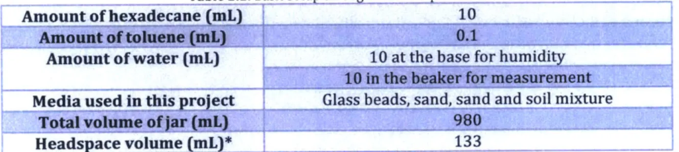
Given the conditions explained above, the various parameters of the experiment can be summarised in the following table:

Table 2.1: Basic setup throughout the experiment

Amount of hexadecane (mL)

Amnount of water (mL) a h aefrhmql

Media used in this

project

Headspace volume(mL)*

133

* Headspace volume has been accounted for in the total volume of the jar

Therefore with this setup, the aim of the experiment is to be able to accurately quantify the amount of COC in the soil gas. To achieve that, a mathematical model for the physical model was developed to estimate the concentration of COC (represented by toluene) in the soil gas prior to the measurement. In addition, the water-based measurement serves as a comparison of the results obtained by the PE passive sampler.

Chapter 3: Experimental details

3.1 Apparatus and chemical handling

All chemical solvents used were of Ultra Resi-analyzed grade from J.T. Baker. Water used

were 18ME1 high quality water that was treated by the system from Vaponics (Model: Aries). Prior to dispensing, the water is UV-treated and filtered with filter pore size of 0.22 pm. 18M(Q water will henceforth be simply described as "water" unless otherwise stated.

Standard laboratory glassware was used and first washed with water, then rinsed with methanol and then with acetone before being dried in the oven at 60 'C.

3.2 Properties and the treatment of PE

PE used in this experiment was commercially available heavy duty "Plastic Sheeting" from Film-Gard with a 4 mil thickness (101.6 ptm). The PE sheets were cut to smaller size of varying mass between 0.1 g and 0.6 g and treated according to the method adopted by Apell

and Gschwend. PE was soaked in dichloromethane twice for 24 h each and then in methanol twice for 24 h each.12 Finally they were left in water only to be taken out for use prior to the start of each experiment.

3.3 Properties and treatment of media

Glass beads of approximately 5 mm in diameter were obtained from teaching laboratory in Parsons Laboratory, Massachusetts Institute of Technology. They were soaked in 2 M HCl for 48 h and then rinsed with water twice before leaving them to air dry.

Sand used in this experiment was commercially available "Premium Play Sand" from Quikrete. The bag of sand was transferred into a large glass jar that is approximately 10 L in volume. It was then placed on a single level, 12 bottle roller (Technical Development

larger sand grains tend to settle to the bottom after transfers. Prior to loading into the experimental setup, a visual inspection was done to ensure that no large pebbles were loaded into the experimental jar.

Contaminated soil from an industrial site was collected by coring and mailed to the laboratory in air-tight glass jars. Prior to use, soil was weighed and transferred to a large bowl to be manually mixed with sand using a spoon in a 1:9 ratio. It was then transferred directly to the experimental setup.

3.4 Instrumentation specifications and methods

Three main analytical instruments were used in this experiment. All three of them employed the basic concept of gas chromatography (GC), with different variations. The first of which involved a GC where 1 pL of sample is injected and the retention time of compounds were registered. The other one comes with a purge and trap system, allowing detection limit 5000 times less than that of the regular GC. The last GC is coupled with a mass spectrometer (GC-MS), where eluent at each retention time was transferred to the mass spectrometer to be fragmented and analysed to allow identification of compounds based on molecular mass. Further methodology and specifications are elaborated below.

3.4.1 Gas chromatography

The gas chromatograph was a Carlo Erba Strumentazione HRGC 5300 Mega Series with a

J&W Scientific capillary column, DB-624 (Agilent Technologies Cat. No. 122-1364), 60 m

length, 1.4 iim film thickness, 0.25 mm inner diameter, with a cold on-column injector and uses a Flame lonisation Detector (FID). The flow rate in the column was 2.5 mL/min. Air flow was kept at 300 mL/min while hydrogen flow was at 30 mL/min. Temperature was

programmed to start at 102 'C and then increased at 10 'C/min from 102 *C until 200 *C, after which the temperature increased at 25 'C/min to 225 *C. Outputs were measured using a Fisher Recordall Series 5000 with a range of 1 mV. Attenuation varied between 32 and 128.

3.4.2 Gas chromatography with purge and trap

The gas chromatograph was a Perkin Elmer Autosystem XL Gas Chromatograph with a

J&W

1.80 ptm film thickness, 0.32 mm inner diameter, with a cold on-column injector and uses a

Flame lonisation Detector (FID). The flow rate in the column was 2.5 mL/min. Air flow was kept at 300 mL/min while hydrogen flow was at 30 mL/min.

The purge and trap was a Tekmar LSC 2000 Purge and Trap with a standby temperature of

35 'C. 5 mL of aqueous solution containing the desired compounds were purged for 5 min.

Desorb preheat temperature was at 200 *C and the desorption was done over 2 min at

225 0C. The bake time was 4 min at 225 *C.

Temperature programme of the GC started at 35 'C with a 1 min hold time. After which it increases at 10 'C/min from 35 'C until 225 *C. Attenuation was kept constant at 2.

3.4.3 Gas Chromatography - Mass Spectrometry

The gas chromatograph was a Hewlett-Packard 6890 Gas Chromatograph with a JEOL GCmate mass spectrometer. The MS was operated in Electron lonisation (El) mode with a m/z range of 35 to 200. The GC is equipped with a J&W Scientific capillary column, DB-624 (Agilent Technology Cat. No. 123-1364) 60 m length, 1.80 pm film thickness, 0.32 mm inner diameter, with a cold on-column injector and uses a Flame lonisation Detector (FID). The

flow rate in the column was 2 mL/min. Temperature programme started at 35 *C and increased at 3 *C/min from 35 *C until 125 'C. It was then increased to 10 *C/min until 225 *C.

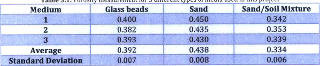
3.5 Measurement of porosity

Porosities of glass beads, sand and the soil/sand mixture were each measured. The values were obtained by filling 50 mL of the respective medium in a 100 mL graduated measuring cylinder (to the 50 mL marking) with the mass of the dry solids measured. Acetone was then added to the 60 mL mark and the combined mass of acetone and the medium was measured. The difference in mass (denoted by Md) would be the mass of acetone that occupied the top 10 mL (without the medium) and acetone that occupied the pore spaces in the 50 mL of medium. Finally, porosity of medium i (<p) was calculated using:

Md_-Pacetone-10 (3.1)

50

pacetone is the density of acetone (using the value at 25 'C which is readily available, assuming negligible difference with density at actual room temperature of 22 *C) in [g/cm 3]. This was

repeated three times for each medium (Table 3.1).

Table 3.1: Porosity measurement for 3 different types of media used in this project

Medium Glass beads Sand Sand/Soil Mixture

2 0.382 -- 0.435 0.353

Average 0.392 0.438 0.334

Standard Devlalgoit AO-7 u0 .006

This measurement neglected the possibility of any sediment settling effects where the medium may rearrange itself slightly upon the addition of acetone.

3.6 Generic passive sampling experimental methods

The experimental setup (Figure 2.1) was left to sit for 24 h for the toluene to reach the equilibrium concentration between all phases (in hexadecane, water and air) within the jar. Following which a PE is inserted into the medium in the jar and sealed for another 24 h for the PE to absorb the toluene from the soil gas. At the end of 24 h, the PE is removed for analysis via a water extraction (see below). A negative control is also used whereby the PE is inserted and taken out immediately for analysis.

3.6.1 Experiment with glass beads

The first experiment was carried out with glass beads. This removed the factor of the presence of organic carbon in the model as glass does not have affinity for toluene. With parameters of the experimental setup obtained (Table 2.1) together with values of constants for toluene (see Appendix), an estimation of the concentration of toluene in air, water and hexadecane was made. This was done by considering the fraction of toluene in the air:

f - (3.2)

fi,a ~~ Ai,b+Aic Ai,a Ai,a

where At; is the amount of chemical i in medium

j.

Table 3.2: Fraction of total toluene and concentration in each phase in experimental jar with glass beads. - lg

KHA was 3.33 for toluene and - ig Kaw was 0.6.15 Both values were taken at 25 C. Room temperature measured was 22 'C. Temperature effect was assumed not to be significant in the estimation of the toluene concentration

for the mathematical model

Phase Air Water Hexadecane

Volume of each phase 435 20 10

(mgL)I

3.6.2 Experiment with sand

Following the experiment with glass beads, the procedures were repeated with sand, a medium that is able to better represent soil than glass beads would. Using the same equation as above (Equation 3.2), the estimates for the various concentrations were found

(Table 3.3).

Table 3.3: Fraction of total toluene and concentration in each phase with sand

Phase Air Water

Hexadecane-Volume of each phase 474 20 10

JmL)

in each phase 3.6 84-40:

3.7 Water extraction of COC from PE

After the PE was removed from the experimental setup, it was placed in a 60 mL BOD bottle filled with water. The bottle was capped and then submerged into a container filled with water and left to sit on a reciprocating shaker table (VWR Advanced Orbital Shakers Model

10000, 60 rpm) for 72 h to allow desorption of toluene from the PE into the water. No air

spaces were present as the bottles were sealed to prevent partitioning of toluene into the air spaces, which may cause inaccuracies in the data acquisition. Upon equilibration, the

water was used in various analytical tests to determine the concentration of chemicals in the water.

Once the concentration of COC in water at equilibrium (Cw,eq) was obtained, it was used to back calculate the initial amount of COC in the PE (CPE,org). This was done by calculating the

concentration of COC in PE inside the BOD bottle (CPE,eq) at equilibrium:

CPE,eq = KPEWCW,eq (3.3)

The original concentration of COC in PE is then derived using the mass of the PE (MPE) and

volume of the BOD bottle that was used in the extraction (VBOD):

CPr = CPE,eqMPE+CW,eq VBOD

Er _MPE

With that, the concentration of toluene in the soil gas (Cair) is related by:

Cair = CPEorg (3.5)

KPEA

The Cair obtained could then be compared against the estimated concentration of toluene

from the mathematical model.

3.8 Preparation of standards

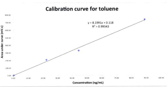
Standards were prepared in order to determine the concentration of the COC (BTEX -benzene, toluene, ethyl-benzene, xylenes) during the experiment. The COC was added in excess to water and shook for 2 min to allow the maximum amount of the COC to dissolve in water. It was left standing to allow phase separation between the aqueous and organic layer for 1 h. The aqueous layer was then removed and diluted accordingly to achieve the desired concentration. Solutions of different concentrations were prepared and were then used to generate a calibration curve for the GC and the purge and trap. The area under the curve at each retention time from the chromatogram obtained from sample analysis can then be

translated into a value that represents the concentration of COC in a water sample using the calibration curve (Figure 3.1).

Calibration curve for toluene

EU a' &W00 7000 O y 8.1991x + 0.118 R' = 0.99343 600 00 40000 4W00 X 200 00 00.00 O00 000 1000 20 00 30,00 40.00 50.00 6000 1000 WOO 9000 100 00 Concentration (ng/mL)

Figure 3.1: Example of a calibration curve for toluene when using the purge and trap. Method of measurement was the same as measuring a sample as described in section 3.4.2.

The calibration curve relating the area under the curve at each retention time on the chromatogram and concentration follow a linear relationship given byy = mx + c, wherey is

the area under the curve in [mV.s] and x is the concentration in [ng/mL]. The response factor, m, typically ranged between 5 to 10 with units of [mV.s.mL/ng].

3.9 Precision of results

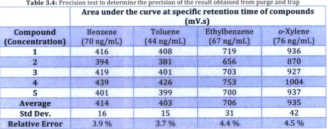
In order to verify that the results were reproducible, multiple replicates were done to evaluate the method's precision. The BTEX solution was prepared similarly to the preparation of a standard described previously (section 3.8) and analysed using the purge and trap (Table 3.4).

Table 3.4: Precision test to determine the precision of the result obtained from purge and trap

Area under the curve at specific retention time of compounds (m

~s)

Compound, Be ne T uene!.'ybnzn o- yleae

1

408

719

936

3 419 401 703 927

5 401 399 700 1 937

Std Dev. 16 15 31 42

Relative Error 3.9 %% 4A %/ _ _4.5,%

Using the result obtained here, the purge and trap data has a relative standard deviation of approximately of 4 % of the average.

Chapter 4: Results and Discussion

4.1 Experimental jar with glass beads

The experiments were carried out by placing the PE into the experimental setup for 24 h and removed thereafter for water extraction. The experiment was repeated twice on two independent setups. Using the toluene concentration from the water in the BOD bottle at equilibrium (Cw,eq), toluene concentration in the soil gas (Cair) was back calculated using

Equations 3.3 - 3.5.

The water-based measurement was also taken and compared against the measurements from the PE. This was done by measuring the concentration of toluene in the beaker of water (Cheaker) at the top of the experimental setup (Figure 2.1). Cair is calculated by using

Equation 2.1. Both Cair derived from the two methods of measurements were then tabulated (Table 4.1).

Table 4.1: Estimated and measured concentration of toluene in soil gas using the PE passive

samplin method and also usin the water-based measurement for the experiment with glass beads

Repeat

Estimated*

Measured soil gas

Measured soil gas

soil gas

concentration from

concentration from

water-concentration

PE passive sampler

based measurement

2 3.34 5.73 6.10

* see appendix for derivation of estimated concentration of toluene in soil gas

Measured soil gas concentration from both methods of measurement showed to be an overestimation of the value derived from the mathematical model of the experimental jar. This implied that more toluene were leaving the pure phase hydrocarbon into the other phases present. This could mean that the partitioning constant of toluene between the air and hexadecane layer (Kah) was not representative at this concentration. The value Kah assumed interaction between hexadecane and toluene in an infinite dilution condition. In the experiment, approximately 1 % of toluene was present in the hexadecane phase and

thus the concentration of toluene in hexadecane may result in non-ideal mixing due to the difference in the shape of the molecules despite similar van der Waals forces of attraction.

Despite the difference between the estimated and measured result, the results had shown that both methods of measurement were consistent with each other. Both forms of

measurement gave results that were approximately twice as much as the estimated value. While the partitioning constant between air and PE or PE and water were experimentally obtained from Liu, Henry's law that describes the partitioning constant between air and water have long been established. This showed that the use of PE is a reliable source of measurement of concentration of COC in the air.

4.2 Experimental jar with sand

With the confirmation of consistency between the two methods of measuring concentration of toluene in the air, the next step would be to use a medium that resembles soil more so than glass beads. Sand was used as a medium in this part of the experiment.

PE were also inserted into the experimental setup filled with sand and taken out for extraction 24 h later. This was done twice over two independent setups. The water-based measurement was also carried out. Concentration of toluene in the soil gas derived from the PE passive sampler was calculated using the same equations (Equation 3.3 - 3.5). Equation 2.1 was also used to calculate the concentration of toluene in the soil gas derived from the water-based measurement. The results were tabulated and summarised (Table 4.2).

Table 4.2: Estimated and measured concentration of toluene in soil gas using the PE passive

sampling method and also using the water-based measurement for the experiment with sand

Repeat Estimated* Measured soil gas Measured soil gas

soil gas

concentration from

concentration from

water-concentration

PE passive sampler

based measurement

(mg/L

(mg/m

2

3.34

2.93

2.97

* see appendix for derivation of estimated concentration of toluene in soil gas

In contrast to the experiment carried out with glass beads, the results of the experiment with sand showed toluene concentrations closer to the estimated value. However, it is more interesting to note that the measurements from the PE and the water-based approached were also consistent even when the medium was changed to sand. This gave further confidence that PE passive sampling was a reliable method of measurement as it had shown to be consistent across two media. An attempt to quantify concentrations in the soil gas can thus be made.

4.3 Investigation on actual soil

Following the tests in an environment of glass beads and then in sand, a quantitative measurements of the contaminants in the actual soil was made. In initial tests, soil samples were prepared by mixing the contaminated soil and sand in a 1:9 ratio. The physical model was modified by removing the reservoir of toluene in hexadecane (Figure 4.1).

Head space for ease of opening and closing Beaker of water for water-based measurement Sand/Soil mixture Water at the base to provide 100 % humidity

Figure 4.1: Modified setup for soil/sand mixture. No reservoir needed as the contaminants were present in the soil itself

4.3.1 Identification of compounds

The same procedures were carried out - PE was inserted into the soil/sand mixture and left for 24 h before removing it for water extraction. However, instead of analysing the water extract immediately, 50 mL was transferred and 1 mL of pentane was added and shook for 2 min to allow transfer of the organic compounds from the aqueous layer to the organic layer. The pentane extract was then analysed using the GC-MS. Following the results obtained, it is possible to conclude that these various compounds were present:

Table 4.3: Retention times and corresponding identity of compounds

Retention time (min:sec) Compound Structure

7:58 Toluene

11:30

H3C

_________CH ₃

12:10 o-Xylene

Given that the C2-benzenes have different boiling points, they can be identified by correlating the boiling point with retention times. As a result, it is also possible to identify the C3 to C5-benzenes. Their approximate retention times under this temperature programme were tabulated (Table 4.4).

Table 4.4: Approximate range of retention times for higher order aromatic hydrocarbon

Retention time range

Group of compounds

General Structure

(min - min)

13.;

444

0-benienem

Therefore with majority of the contaminants consisting of aromatic hydrocarbons, BTEX were chosen to be the group of COC. In this thesis, only o-xylene was used.

4.3.2 Quantitative analysis of contaminants in soil

With the focus on quantifying the amount of BTEX in the soil, the experiment was repeated with the same setup. PE was inserted into a new soil/sand mixture and removed after 24 h for water extraction. Both water extraction and water-based measurements were used and were analysed using the purge and trap. By comparing the area under the curve at each retention time against the calibration curve of the respective compounds for both methods, the Cair of each of the compounds were back-calculated using the same steps as previously described. After which the results were tabulated (Table 4.5).

Table 4.5: Estimated concentration of soil gas from PE and the water-based measurement in actual soil/sand mixture. Constants related to the compounds can be found in the appendix

rnmnnund Benzene I Toluene Ethvlbenzene o-Xvlene

Estimated

concentration in soil 31 gas from water-based

measurement

(pg/L)

In contrast to the controlled experiment where the PE water extract and the water-based measurement gave consistent results, the concentration of BTEX in an actual soil sample from the same two independent methods of measurement gave rise to very different results.

One possible reason for the large discrepancy in the result could be the possible presence of biodegradation. The water-based measurement was carried out almost a week after the PE passive sampling was done. This may have led to a decreased concentration of BTEX during that time frame.

In the experiment with glass beads and sand, it was assumed that there were no bacteria present in significant quantities that would cause any discrepancy between the results obtained from the two methods. This is evident in the results as shown in the previous

sections.

In contrast to glass beads and the sand, the actual soil sample was taken from the site at depth 2.3 to 2.8 m below surface level. This could indicate an environment that was lacking in oxygen required to facilitate aerobic degradation of the BTEX. It is possible that only anaerobic degradation was occurring, or no degradation was occurring. In the process of collecting these soil samples, they had been dug up to surface where oxygen is abundant and thus might have had reintroduced oxygen into the soil samples. Furthermore during the process of handling the soil sample, it has been constantly exposed to oxygen and therefore the rate of biodegradation might have increased rapidly after the initial measurement.

In order to verify that biodegradation is present, further studies would be required. A possible way would be to drive off the contaminants in the soil, and then a deliberate attempt to contaminate the soil sample. Presence of aerobic degradation can thus be

observed by monitoring the rate of disappearance of the contaminants. However this is beyond the scope of this project which will not be discussed further.

4.3.3 Estimation of concentration of other compounds

Currently the results obtained from the two different measurements are not consistent. However once proven successful, it is possible to obtain a rough estimation of the extent of pollution by the other compounds.

This can be achieved by using the linear relationship generated by Liu to obtain an estimate

of the KPEA/KPEW for C3, C4 and even C5-benzenes. It describes the linear relationship

between log K.w and log KPEW. Estimates of log K0w can be obtained using the method

developed by Meylan and Howard.19 The straight chain isomer of the C3, C4 and

C5-benzenes (ie. proylbenzene, butylbenzene and pentylbenzene) were used in the estimation of log Kow, which was then used as a representative value for its group of compounds. In the absence of a calibration curve for these compounds, a generaly = mx formula will be used to

estimate the concentration of COC in water based on the area under the curve at respective retention times on the chromatogram. The response factor, m was assumed to be 10 mV.s.mL/ng for all groups of compounds for this estimation. The concentration of these compounds in the soil gas in presence of the PE sampler were then estimated and tabulated

(Table 4.6).

Table 4.6: Estimates of concentration of these groups of compounds in the soil gas from the PE passive sampling. Constants used and concentration of the water extract at equilibrium can be found in the appendix.

Group of compounds C3-benzene C4-benzene CS-benzene

-C3H7 -C 4 9 -C111

Chapter 5: conclusion and future work

5.1 Conclusion

Quantitative analysis of COC in the air using PE passive sampling proved to be consistent with analysis from the water-based measurement when the level of contaminations was known. The water-based measurement relied on Henry's law, which is a well established concept and thus deemed to be a reliable method for cross-referencing. This showed that PE passive sampling has the potential to accurately quantify concentrations of COC in air.

Aromatic hydrocarbons from benzene to C5-benzenes were identified to be present in the actual soil sample via GC-MS. BTEX was then chosen to be analysed and quantified given their ubiquitous presence in fuel spills. However, concentrations of BTEX from both methods of measurements were not consistent, possibly due to the action of biodegradation. Biodegradation however, was not present in the controlled setup. Nonetheless, in the absence of established literature values of certain parameters, estimates from linear relationship can be used to calculate a rough concentration of COC in air based on just the molecular mass of the COC.

5.2 Future work

5.2.1 Pentane extraction instead of water extraction of chemicals

The current method relies on the partitioning of compounds between air and the PE during the data acquisition, and then between the PE and water for water analysis. Therefore this is dependent on the partitioning constants of the chemicals between air and the PE and then between PE and water. With PE being an organic material, it would favourably absorb the organic compounds given similar forces of attraction. However due to that reason, the

organic compounds may favourably decide to stay within the PE and not be desorbed into the water during the water analysis. This has implication on the MDL of different compounds, especially if a compound is present in low concentration and is also toxic in very low concentration in the environment.

Thus there were attempts throughout this project that looked into the possibility of doing a pentane extraction. PE removed from the experimental jar were submerged into pentane instead of water. However there were many issues with the inconsistency in the methodology and results obtained. One particular problem was preventing the evaporation of pentane in a capped glass vial. The difficulty in handling pentane due to its volatility makes it a challenge to carry out pentane extraction. However with further improvements

on the methodology, it might be a possible option.

5.2.2 Performance reference compounds (PRCs)

It was mentioned earlier in Chapter 1 that the use of PRCs would be a good way of measuring the extent of equilibrium reached. Jensen mentioned in his thesis (personal communication) that the model predicts a 90 % equilibrium when the PE (2 mil thickness) has been inserted in the soil for 12 h.2 In this project, the PRC (chlorobenzene) was pre-loaded into the PE. At the end of each experiment, GC analysis revealed that 95 to 100 % of the chlorobenzene had diffused out of the PE. Each PE was left inside the experimental setup for 24 h. Therefore it showed that near equilibrium conditions were achieved after 24 h. However, PRC measurements were not further explored in this project in the interest of

Further investigations can be carried out in the form of a timed course, where PE can be inserted into the setup but removed at regular intervals in order to draw the timed course showing the percentage of PRC remaining in the PE.

The measurements of the PRC out of the PE would be exceptionally useful information as it gives a clearer picture about the deployment time of the PE in the soil. With current literature showing that PRCs are good measurements of extent of equilibrium especially in the sediment, this will give end users (eg. consultants) confidence that they can get quick results, in contrast to existing technologies that may take several days or even weeks to acquire data. Thus there is a strong motivation to look into this.

5.2.3 Measurement of biodegradation and field testing

Currently although the PE passive sampling method and the water-based measurement have shown to be consistent in the controlled setup with glass beads or sand, it has failed to produce that consistency when measuring the actual soil. It was mentioned that biodegradation might be a reason for this inconsistency. Thus once possible way forward would be to verify this hypothesis.

Following which, modifications to the model can be made if necessary, and then together with the probe prototype designed by Jensen, which currently consist of a long rod with a retract-a-tip system at the end that can be driven into the soil by hand2, a field testing can be carried out.