Publisher’s version / Version de l'éditeur:
Proceedings of the International Workshop on Spoken Lanuage Translation
(IWSLT-2011), 2011-12
READ THESE TERMS AND CONDITIONS CAREFULLY BEFORE USING THIS WEBSITE. https://nrc-publications.canada.ca/eng/copyright
Vous avez des questions? Nous pouvons vous aider. Pour communiquer directement avec un auteur, consultez la
première page de la revue dans laquelle son article a été publié afin de trouver ses coordonnées. Si vous n’arrivez pas à les repérer, communiquez avec nous à PublicationsArchive-ArchivesPublications@nrc-cnrc.gc.ca.
Questions? Contact the NRC Publications Archive team at
PublicationsArchive-ArchivesPublications@nrc-cnrc.gc.ca. If you wish to email the authors directly, please see the first page of the publication for their contact information.
NRC Publications Archive
Archives des publications du CNRC
This publication could be one of several versions: author’s original, accepted manuscript or the publisher’s version. / La version de cette publication peut être l’une des suivantes : la version prépublication de l’auteur, la version acceptée du manuscrit ou la version de l’éditeur.
Access and use of this website and the material on it are subject to the Terms and Conditions set forth at
Semantic smoothing and fabrication of phrase pairs for SMT
Chen, Boxing; Kuhn, Roland; Foster, George
https://publications-cnrc.canada.ca/fra/droits
L’accès à ce site Web et l’utilisation de son contenu sont assujettis aux conditions présentées dans le site LISEZ CES CONDITIONS ATTENTIVEMENT AVANT D’UTILISER CE SITE WEB.
NRC Publications Record / Notice d'Archives des publications de CNRC:
https://nrc-publications.canada.ca/eng/view/object/?id=e86752cf-7b89-4f65-baa1-8a31a9d762b6
https://publications-cnrc.canada.ca/fra/voir/objet/?id=e86752cf-7b89-4f65-baa1-8a31a9d762b6
Semantic Smoothing and Fabrication of Phrase Pairs for SMT
Boxing Chen, Roland Kuhn and George Foster
National Research Council of Canada, Gatineau, Québec, Canada
First.Last@nrc.gc.ca
Abstract
In statistical machine translation systems, phrases with similar meanings often have similar but not identical distributions of translations. This paper proposes a new soft clustering method to smooth the conditional translation probabilities for a given phrase with those of semantically similar phrases. We call this semantic smoothing (SS). Moreover, we fabricate new phrase pairs that were not observed in training data, but which may be used for decoding. In learning curve experiments against a strong baseline, we obtain a consistent pattern of modest improvement from semantic smoothing, and further modest improvement from phrase pair fabrication.
1.
Introduction
The translation model component of phrase-based statistical machine translation (SMT) systems (the “phrase table”) consists of conditional probabilities for phrase pairs observed in the training data. However, estimation of these probabilities is hindered by data sparseness; thus, phrase table smoothing techniques are often applied [1].
The most popular phrase table smoothing approach is lexical weighting, where the conditional probabilities for the phrase pair made up of source-language phrase s and target-language phrase t are smoothed with probabilities for alignments between individual words inside s and t. Two different lexical weighting techniques are given in [2,3].
In this paper, we explore a different approach to phrase table smoothing which is based on paraphrases. Our work extends a new type of smoothing described in two recent papers [4, 5]. This type of paraphrase-based smoothing differs from earlier types described in the literature because it exploits “endogenous” [5] information – i.e., the original training data for the SMT system – rather than external data such as additional parallel corpora.
In [4], phrases in the same language that are close together, according to metrics based on distributional similarity of translations into the other language, are hard-clustered. For instance, the English phrases “kick the bucket”, “die” and “expire” might have similar but not identical distributions of French phrase translations; when these English phrases are clustered together, the pooled distribution is more informative than the individual ones. The “phrase clusters” in each language are used offline to generate estimates PPC(s|t) and PPC(t|s) for source and target phrases s
and t, providing two new features for the decoder.
Generation of these hard clusters relies on a computationally intensive, iterative process. A starting language (which could be the source or target language) is picked. A small amount of clustering is carried out in that language. That is, starting with a situation in which each phrase in the language is its own cluster, phrases that are
close together are merged into the same cluster. This affects the distances between phrases in the other language, since phrases in the first language that are now in the same cluster are treated as if they were identical. A small amount of clustering is carried out in the second language, then again in the first language using the altered distances for that language, and so on.
Max [5] describes an online technique that relies on context in the input text to weight information from paraphrases. This technique increases the estimated P(t|s) if paraphrases of s were translated as t in contexts in the training data that are similar to the context of the current instance of s in the input text.
Some other work on paraphrases for SMT based on external data include [6] which extracts paraphrases from external parallel corpora, and [7] which showed that this kind of paraphrase generation could improve SMT performance. [8] derived paraphrases from external monolingual data using distributional information.
In this work, we first extend [4] by replacing hard clusters with a softer version in which each phrase’s distribution is smoothed with the distributions of its nearest neighbours. We call this semantic smoothing (SS); it is more accurate, and requires less computation, than hard clustering.
A more dramatic advance over earlier work is that we “fabricate” phrase pairs that weren’t seen in training data. In [7], phrase pairs (s,t) may be fabricated because s occurs in the input text but cannot be found in the phrase table. REMOOV [9] does not use paraphrases, but fabricates phrase pairs with OOV source by modifying observed Arabic source phrases using rules that capture frequent misspellings, transliteration variations, etc. Self-training [10] also does not use paraphrases; it learns variations of existing phrase pairs from the N-best output of the system on new source-language input.
Our fabricated phrase pairs are different: we apply paraphrase information to generate new translations for some phrases that already have translations in the phrase table, using other information in the phrase table.
2.
Semantic Smoothing
In this section, we describe how, for a given phrase in the source or target language, we find the other phrases in the same language that are its closest neighbours in a kind of semantic space (2.1-2.3). Then, we explain how the conditional translation probabilities for the given phrase are smoothed with information from those neighbours (2.4). Finally, we explain “phrase pair fabrication”: generation of some phrase pairs that weren’t observed in the original data, but which are judged to be plausible according to the smoothed probabilities (2.5).
2.1. Metrics
We use a metric from [4] to compute the semantic distance between two phrases in the same language: the so-called Maximum Average Probability Loss (MAPL) metric.
Each phrase is represented by the vector of its counts of co-occurrence with phrases in the other language, transformed by a modified version of tf-idf [11]. Unlike the original tf-idf, this transformation is not based on word-document co-occurrences, but on phrase-phrase co-occurrences in the phrase table. For example, for source-language phrases, each co-occurrence count #(s,t) between a source phrase s and a target phrase t is multiplied by a factor reflecting the information content of t. Let #diffS be number of different source-language phrases in the phrase table, and let #[t>0] for a target phrase t be the number of different source phrases s that co-occur with t. Then let
])
0
t
[
/#
log(#
)
t
s,
(
#
)
t
s,
(
'
#
=
×
diffS
>
S . Similarly, priorto target-language phrase distance computation, let
])
0
s
[
/#
log(#
)
t
s,
(
#
)
t
s,
(
'
#
=
×
diffT
>
T where #diffT isthe number of different target-language phrases in the phrase table.
Let two phrases u and v in one language be shown as vectors with dimension D (= # of different phrases of any length in the other language):
u = {u1, u2, …, uD}
v = {v1, v2, …, vD}
where ui and viare the transformed phrase co-occurrence counts derived from the formulas above. For instance, to represent phrase u in the source language, ui is the transformed count of co-occurrences of u with the ith target phrase ti: ui = #S’(u,ti).
To define MAPL, first let:
)
log(
...
)
log(
)
(
1 1×
+
+
×
=
i i D D i iu
u
u
u
u
u
I u
, (1))
log(
...
)
log(
)
|
(
1 1×
+
+
×
=
i i D D i iv
v
u
v
v
u
I
u
v
. (2)I(u) measures how well the data in u are modeled by the normalized vector (u1/ iui, …, uD/ iui).
I
(
u
|
v
)
measures how well the counts in v predict the distribution of counts in u. Then Maximum Average Probability Loss (MAPL) is: ) ) | ( ) ( , ) | ( ) ( max( ) , ( = − + − + i i i i v I I u I I MAPL uv u u u v v v u v . (3)Like [4], we multiply the MAPL distance with the Dice coefficient. For u and v in the same language, this is
|
|
|
|
|
|
2
1
)
,
(
v
u
v
u
v
u
+
∩
×
−
=
Dice
(4)where |u| is the number of non-zero entries in u, and |
u ∩
v
| is the number of entries that are non-zero in u and v. This shrinks the u, v distance if they have similar patterns of non-zero counts.Again following [4], we used a “maximum common word sequence” (MCWS) edit distance. This is defined as
)
(
)
(
))
(
(
2
1
)
(
v
u
v
u,
v
u,
len
len
MCWS
len
Edit
+
×
−
=
. (5)where len() returns the number of words and MCWS(u,v) is the length of the longest continuous substring that is in both string u and string v.
Thus our distance function was MAPL×Dice×Edit. We experimented with some other distance functions on development data (e.g., with products involving cosine distance) but never found one that worked better than this one. The intuition is that the MAPL term measures how similar the information in the count vectors from the two phrases is, the Dice term gives a bonus if the pattern of non-zero counts for the two phrases is similar (even if the patterns of relative weights for the non-zero counts are very different) and the Edit term gives a bonus if the two phrases have common word sequences.
Important note: the transformations above (e.g., our version of tf-idf) are only applied to distance calculations; the probability calculations below use the original phrase co-occurrence counts.
2.2. Defining nearest neighbours (NNs)
SS differs from [4] in smoothing the distribution for a phrase with the distributions of its at most M nearest neighbours (NNs), rather than with the distributions of its fellow-members in a fixed phrase cluster (disjoint from other clusters). NNs must satisfy a maximum distance criterion, parameterized by a user-defined threshold F. Thus, the NNs are those of its neighbours which are a distance F or less away from it; if there are more than M such neighbours, the M closest to the phrase are chosen.
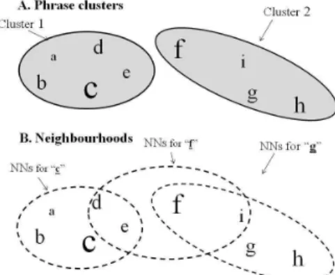
Figure 1: phrase clustering vs. nearest-neighbour semantic
smoothing (SS)
Figure 1 gives an example. Clustering gives two
distributions: one calculated from phrases “a”, “b”, “c”, “d”, and “e”, and yielding cluster probabilities for those phrases, and another calculated from “f”, “g”, “h” and “i” and yielding probabilities for those phrases. By contrast, SS yields a different distribution for each phrase. Figure 1B shows NNs for 3 of the phrases, “c”, “f” and “g” (each of the 9 phrases has its own NN set). Unlike 1A, in 1B a phrase can be involved in calculating more than one distribution: e.g., “e” is involved in the distributions for “c” and “f”. Phrases with many observations have a strong impact on distributions they participate in. E.g., “f” has more observations than other
phrases (hence the large font) and thus strongly influences SS estimates for “g” and itself.
2.3. Rank discounting of counts
The most effective version of SS we tried used distance-dependent discounting of information: it assigns less importance to information from NNs that are far away from the given phrase, on the grounds that their meaning is less similar to that of the given phrase than that of closer phrases. In practice, we used nearness rank rather than exact distance: the phrase itself gets rank 1, the closest other phrase to it gets rank 2, and so on. E.g., to smooth the “g” distribution in
Figure 1B, counts from “g” are unchanged, those from “i”
(the nearest phrase to “g”) are divided by 2, those from “h” (second nearest to “g”) are divided by 3, and those from “f” (third nearest) are divided by 4. The sum of the modified counts yields an estimated distribution for “g”. Discounting reduces the influence of the highly frequent phrase “f” on the smoothed “g” distribution. It would be interesting to experiment with a form of discounting that uses absolute distance instead of rank – we did not have time to explore this possibility.
The details are as follows. Let’s list source phrases in some order s1, …, s|S| and similarly for target phrases t1, ..., t|T|.
Let si = |T|-dimensional row vector of co-occurrence counts
for si = [c(si,t1), … c(si,t|T|)], and let tj = |S|-dimensional
column vector of co-occurrence counts for tj. Let #si = total
count of si, let #tj = total count of tj, and let NNr(si) and
NNr(tj) (with no underscore) denote the rth NN of si and tj
respectively. Let N(si) denote the ordered set of the count
vectors for the NNs of si, N(si) = [si; NN1(si); …; NNk(si)],
0≤k≤M (if k=0 that means there were no acceptable neighbours for si and N(si) = [si]). Similarly, N(tj) = [tj;
NN1(tj); …; NNm(tj)], 0≤m≤M.
Let the “discount-by-rank” scheme above be denoted r(). Let’s construct rank-discounted total count vectors from N(si)
and N(tj): r(N(si)) = si + =
+
k r rr
1)
(
1
1
is
NN
(6) and r(N(tj)) = tj + =+
m r rr
1)
(
1
1
jt
NN
. (7) The count for phrase t inside the r(N(si)) vector isdenoted r(N(si))[t], and the count for phrase s inside the r(N(tj)) vector is denoted r(N(tj))[s]. We denote the totals for
these two vectors as #r(N(si))= tr(N(si))[t] and
#r(N(tj))= sr(N(tj))[s].
Inside the r(N(si)) vector, for a target phrase tj, we can
sum the rank-discounted contributions from its NNs; this is also what we get as the rank-discounted sum of contributions of the NNs of si inside r(N(tj). We denote this quantity
#(r(N(si))∩r(N(tj))) =r(N(si))[tj]+ =
+
k r rr
1)]
(
))[NN
(
(
1
1
j it
s
N
r
=r(N(tj))[si]+ =+
m r rr
1)]
(
))[NN
(
(
1
1
i js
t
N
r
. (8)2.4. Conditional Probability Estimation
We apply formulas in which both estimates benefit from smoothing in both languages. The intuition is that, for instance, the probability of translating the French word “louche” as “seedy” is estimated as the probability of translating “louche” or any of its French synonyms as “seedy” or any of the English synonyms of “seedy”, times the probability of choosing “seedy” from among its synonyms.
Thus, we have ( | ) ( | ( )) ( ( )| ( )) j i i i j i t Ps Ns PNs Nt s P = × and )) ( | ) ( ( )) ( | ( ) | (tj si Ptj Ntj PNtj Nsi P = × . Here, N(si) (for
example) is a fuzzy set of observations that “resemble” si. Let
)) ( r( # ))) ( ( )) ( ( ( # )) ( r( # # ) | ( j j i i i j i t N t N r s N r s N s t s P ∩ × ≈ , (9) )) ( r( # ))) ( ( )) ( ( ( # )) ( r( # # ) | ( i j i j j i j s N t N r s N r t N t s t P ∩ × ≈ . (10)
2.5. Phrase Pair Fabrication
We fabricate phrase pairs that were not seen in the training data but which are assigned high probability by the SS model, and allow the decoder to use them. For each phrase pair (s,t) that is observed in the training data, where s has a set of nearest neighbours (s1’, s2’, …, sk’), and t has a set of nearest
neighbours (t1’, t2’, …, tm’), we add to the phrase table every
pair (si’,tj’) that is not already in it. A fabricated phrase pair
(FP) will be assigned a very small probability ε=10-18 by the relative frequency component of our SMT system, but may receive fairly high scores from SS and from the lexical weighting (LW) features; if an FP does have high SS and LW scores, it is quite possible it may be used for decoding.
3.
Experiments
3.1. System detailsWe carried out experiments on a phrase-based SMT system with a phrase table derived from merged counts of symmetrized IBM model 2 [12] and HMM [13] word alignments. The system has lexicalized and distance-based distortion components. For FPs, the lexicalized distortion components are set to default, averaged values.
The baseline is a loglinear combination with language models, the distortion components, relative frequency estimators PRF(s|t) = #(s,t)/#t and PRF(t|s) = #(s,t)/s and lexical
weights PLW(s|t) and PLW(t|s). The PLW() are based on [3] and
can be computed without alignments inside phrases; Foster et al. [1] found this to be the most effective lexical smoothing technique. In our experiments, SS components PSS(s|t) and
PSS(t|s) are added to the baseline. We set PRF(s|t) and PRF(t|s)
to a small value ε=10-18 for FPs. Weights on feature functions are found by lattice MERT [14], with aggregation of lattices over iterations.
Before doing the experiments described below, we carried out some preliminary CE experiments with FBIS as training data (9.0M target words) and NIST04 and NIST06 as development data to narrow down the exact way in which nearest neighbours are chosen and their statistics used for smoothing (we did not optimize separately for the FE language pair). These preliminary experiments showed that each of the three terms in the distance function
MAPL×Dice×Edit yields a performance improvement, as
does use of the rank discounting described in Section 2.3. The experiments also helped us find a good value for the maximum number M (=10) of neighbours used for smoothing and for the F parameter that determines the maximum distance from the current phrase that a phrase can have, while still being used for smoothing.
3.2. Data
We evaluated our method on Chinese-to-English (CE) and French-to-English (FE) tasks. CE training data are from the NIST 2009 evaluation; all allowed bilingual corpora except the UN corpus, Hong Kong Hansard and Hong Kong Law corpus are used for the translation model (66.5M target words in total). For CE, we train two 5-gram language models: the first on the English side of the parallel data, and the second on the English Gigaword v4 corpus. Our CE development set is made up mainly of data from the NIST 2005 test set; it also includes some balanced-genre web-text from the NIST training material. NIST 2008 is used as the blind evaluation set.
For the FE task, we used WMT 2010 FE track data. Parallel Europarl data are used for training (46.6M target words in total); WMT Newstest 2008 is used as the dev set and WMT Newstest 2010 is used as blind evaluation set. Two language models are used in this task: one is the English side of the parallel data, and the second is the English side of the GigaFrEn corpus.
3.3. Results
Our evaluation metric for all experiments was case-insensitive BLEU [15], with matching of n-grams up to n = 4.
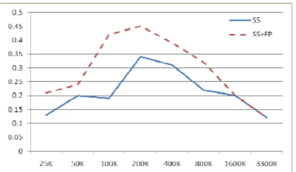
Figure 2: CE BLEU improvement vs. #training sent.
Figure 3: FE BLEU improvement vs. #training sent.
Table 1 : CE BLEU scores on NIST08
Training (#sent.) #phrase pairs Baseline +SS +SS+FP 25K 278K 15.87 16.00 16.08 50K 518K 17.88 18.08 18.12 100K 992K 19.64 19.83 20.06 200K 1.93M 21.27 21.61 21.72 400K 3.78M 22.66 22.97 23.05 800K 7.18M 23.91 24.13 24.23 1.6M 14.06M 25.10 25.30 25.30 3.3M 27.17M 26.47 26.59 26.59
Table 2: FE BLEU scores on Newstest 2010
Training (#sent.) #phrase pairs Baseline +SS +SS+FP 25K 1.12M 20.67 20.79 20.81 50K 2.27M 22.13 22.37 22.41 100K 4.56M 23.36 23.60 23.67 200K 9.12M 24.23 24.54 24.59 400K 18.22M 25.15 25.34 25.39 800K 36.02M 25.8 25.92 25.94 1.6M 70.71M 26.58 26.71 26.71
We evaluated SS and phrase pair fabrication given various amounts of training data. Figures 2 and 3 give BLEU gains on test sets over the baseline; Tables 1 and 2 give more information about the same experiments. As with phrase clustering in [4], the gain is largest for medium amounts of data. “SS+FP” gives a small gain over “SS” alone for small and medium amounts of training. The biggest gain is 0.45 BLEU for “SS+FP” in the CE NIST08 test with 200K training sentences. “SS” helps in all 15 experiments, and “SS+FP” helps further in 12 of 15 experiments.
Are these results statistically significant? Most results in
Tables 1 & 2 are not statistically significant, taken
individually. However, note that (e.g.) each one of the 8 SS results in Table 1, and each one of the 7 SS results in Table 2, shows an improvement over the baseline. Under the null hypothesis that SS has no effect, the probabilities of an improvement or of a deterioration are equal: 0.5. Under the null hypothesis, the probability of seeing these SS results is thus like that of obtaining 15 “heads” in a row in a coin toss.
Table 3: PC vs. SS vs. SS+FP (BLEU scores)
FBIS, CE NIST08 400K, CE NIST08 200K, FE Newstest 2010 Baseline 23.11 22.66 24.23 +PC 23.59 22.90 24.40 +SS 23.70 22.97 24.54 +SS+FP 23.85 23.05 24.59
We also compared SS with phrase clustering (PC). In [4], the largest gains for PC over the baseline are for CE and FE systems trained on 400K and 200K sentence pairs respectively. We compared PC and SS systems trained on the same size data, and on the CE task when trained on FBIS data. As Table 3 shows, SS and SS+FP perform slightly better than PC. Since PC (which involves several iterations of clustering) requires much more computation than SS or SS+FP, the latter appear to be preferable.
3.4. Analysis
Figures 4-7 all pertain to phrase pairs used by the decoder to
build the 1-best output on blind eval (for the parameter settings given above).
Figure 4 and Figure 5 are for systems trained on 200K
sentence pairs (where improvement due to SS and SS+FP was highest). For these figures, “ch” means Chinese, “en” means English, and "fr" means French. Only around 15% of source and target decoding phrases for the CE and FE systems have any neighbours close enough to smooth their distribution – i.e., only a minority of phrase pairs benefit from SS. Only 15.4% of CE and 17.2% of FE decoding phrase pairs in these systems have SS estimates that are different from RF (relative frequency) ones. (The proportion of phrases and phrase pairs with at least one NN was even lower in the original phrase tables for these systems: less than 10% of all phrases in CE and FE phrase tables, with 12.7% of CE and 15.8% of FE pairs in the tables having SS estimates different from RF).
To summarize: for both CE and FE, less than 10% of source or target phrases in the phrase table, and around 15% of source or target phrases used to produce 1-best output are smoothed by SS. Thus, SS has a modest effect because it only smoothes a few phrases - most phrases don’t have NNs because their neighbours are too distant.
Figure 4: CE - number of NNs per decoding phrase
Figure 5: FE - number of NNs per decoding phrase
Figure 6 shows the number and percentage of phrase
pairs chosen for decoding that are fabricated. The numbers are tiny: the maximum is 185 decoding FPs in 25K CE (0.64% of the 28,837 phrases used for decoding by this system). The chosen FPs come from a large candidate pool: FPs were 0.31%-0.13% of pairs in the CE phrase table (the proportion shrinks as training data grows from 25K to 3.3M) and 0.44%-0.16% of pairs in the FE system (the proportion shrinks as training data grows from 25K to 1.6M). For both CE and FE, the number and proportion of FPs used for decoding goes down as the training data grows, even though Figures 2 & 3 show the FPs help most around 100-200K. FPs are used more by CE than FE, perhaps because of noisier CE training data.
Figure 7 shows the distribution of fabricated phrase pairs
(s,t) by number of observations of s. The most common case for both CE and FE is fabrication of a new translation t for an
s that has been observed twice in the training data.
Figure 6: % of decoding pairs that are fabricated vs. #training
sentences.
Figure 7: proportion of decoding FPs by # true observations
of s (CE & FE both trained on 200K sent.)
3.5. Examples
Though we have not performed quantitative comparisons of the outputs of our baseline systems with those incorporating semantic smoothing (SS) and fabricated phrase pairs (FPs), we have carried out qualitative comparisons, and drawn some tentative conclusions.
Table 4 shows some examples of the impact of SS on our
French-English system. The first example is the ideal case: the baseline system (BL) outputs an incorrect, literal translation of the French term “systèmes d’exploitation” (“systems of exploitation”) while the system with SS outputs the correct translation, “operating systems”. Both the translation quality (combined fluency and adequacy as assessed by French-English bilingual colleagues of the authors) and the BLEU score go up. The second example contains perhaps the
commonest type of change introduced by SS: a word substitution which neither improves nor degrades the quality of the translation as assessed by humans. Here, the word “restricted” output by the baseline is replaced by “limited” in the SS version. In this example, BLEU goes down because the reference happens to agree with the baseline in using “restricted”, but we observed just as many cases where neutral substitutions increased BLEU. In the third example, a rather complicated French idiom is translated incorrectly by the baseline, correctly by the system with SS. BLEU happens to go up, even though the SS system’s translation is somewhat different from the reference one.
The last example is perhaps the most interesting. Here, the SS system generates a translation that is worse than the baseline’s according to both human assessment and BLEU. The system has fabulated a “we” subject for the second half of the sentence that isn’t in the source sentence (both the baseline and the SS system fabulate a “he” subject for the first half).
Note that the incorrect second half of the SS output in the last example is more fluent than the corresponding part of the baseline output. This is what we’ve observed for most changes made by SS. Whether the differences introduced by SS are right, neutral, or wrong compared to the baseline (they are usually either right or neutral), they are typically in the direction of greater fluency. This is true for CE as well as for FE (though we don’t have room to present CE examples here). This makes sense: SS has its largest effect (see Fig. 7) on rarely observed phrases in the source language, causing them to be translated similarly to their common synonyms – i.e., less idiosyncratically and more fluently.
We also looked at examples where an SS system that allows FPs had different output than that of an SS system without FPs. In one case (involving a very long sentence), the baseline and the SS system both had trouble with the French past participle “apparu”, meaning “appeared” or “emerged”. Where the reference has “when it emerged”, the baseline and the SS system both had the bizarre “after it is tripoli” (presumably originating from bad phrase alignment). The system with FPs corrected this to “after it is apparent”, correctly hypothesizing that “apparent” is an acceptable translation for “apparu”. In another French-to-English
example we saw, neither the baseline nor the SS system could translate “joueront” (“they will play”), yielding the awkward “they will an important role” where the reference has “they will play an important role”. The system with FPs generates “they will have an important role” – not perfect, but much more fluent.
4.
Conclusion and Future Work
We have shown that semantic smoothing (SS) of SMT phrase pairs improves performance for two language pairs. It may perform slightly better, and is certainly much less computationally expensive, than a previous hard clustering approach [4]. Improvement occurs when SS is only applied to “seen” phrase pairs; there seems to be a slight further improvement when the decoder can also use “fabricated” phrase pairs (SS+FP). Just as with phrase clustering in [4], the improvement is largest for medium amounts of training data. The explanation given in that paper was that smoothing of this type has the most impact on phrases that have enough observations that their neighbours can be located accurately, but not so many that smoothing is unnecessary. That explanation would make sense here too.
“Fabrication” did not have a major impact in our experiments, but it is a logical extension of any kind of smoothing (not just SS): if probability mass can be moved from one seen phrase pair to another, it can also be moved from seen pairs to “holes” in the source-target co-occurrence matrix. The more phrase pair probability estimators there are in a system, the less important the RF estimators are and the safer it is to decode with FPs. In this paper, lexical models “vouched for” some FPs. Adding syntactic or other models might make FPs more important, because it would make it easier for the system to distinguish between bad, dangerous FPs and those that are plausible according to other evidence.
As was mentioned in the discussion of Figures 4 & 5, less than 15% of the phrases used for decoding are affected by SS. This suggests that the modest improvements seen in Figures 2 & 3 may be the result of fairly substantial gains on this small subset of the phrases (and, of course, no gain at all on the
Table 4: SS - sample output for FE system. BL in first column means “baseline”; QUAL in the column Impact means
human assessment; + means positive improved, = means neutral, - means negative impact.
English translation Impact
1. Ref BL SS
… a smartphone with two operating systems .
… a smartphone equipped with two systems of exploitation . … a smartphone equipped with two operating systems .
QUAL+, BLEU+
2. Ref BL SS
access to many web sites is restricted . access to many websites is restricted . access to many websites is limited .
QUAL=, BLEU-
3. Ref BL SS
it is not for want of trying . this is no fault to try . this is not without trying .
QUAL+, BLEU+
4. Ref BL SS
a nice evening , but tomorrow the work would continue .
he had spent a pleasant evening but tomorrow should resume work . he had spent a pleasant evening but tomorrow we should go back to work .
QUAL-, BLEU-
others). Thus, our priority must be to find ways of applying SS to a much larger proportion of phrases.
We now believe that the main reason most phrases don’t have neighbours that are sufficiently close for SS to be profitably applied is polysemy. An invented example: suppose the two English phrases that are closest to “red” are “scarlet” and “Marxist”. If “red” is smoothed with both of these, translations of “red” that should convey the colour sense may inappropriately convey the ideological sense, and vice versa. With our current approach, we end up choosing ultra-cautious parameter settings in which only phrases that have exactly the same sets of meanings are smoothed together, to avoid this sort of semantic pollution. It would be better to distinguish different senses of a phrase, so that (e.g.) the colour sense of “red” could be smoothed with statistics from “scarlet”, and the ideological sense smoothed with statistics from “Marxist”. The approach in [5] achieves this; thus, a hybridization of the two approaches seems like a promising direction. Note that our approach has advantages that the one in [5] lacks – for instance, we smooth both P(s|t) and P(t|s), while the other approach only smoothes P(t|s) – so a hybrid approach would probably be an improvement over both parent approaches.
SS could be improved in several other ways, including significance pruning [16] prior to SS, or a better edit distance (e.g., weighted Levenshtein). One could apply principal component analysis (PCA) or related techniques to infer hidden structure in the bilingual semantic space, thus exploiting information from the neighbours of the neighbours of a phrase. External linguistic resources could be used to find more, better NNs for phrases. Finally, SS could be reformulated as a feature-based model, so the space of alternatives (metrics, number of NNs, discounting, etc.) could be explored more systematically.
5.
References
[1] G. Foster, R. Kuhn, and H. Johnson. “Phrasetable smoothing for statistical machine translation”. Proc. EMNLP, pp. 53-61, Sydney, Australia, July 2006. [2] P. Koehn, F. J. Och, D. Marcu. “Statistical Phrase-Based
Translation”. Proc. HLT-NAACL, pp. 127-133, Edmonton, Alberta, Canada, May 2003.
[3] R. Zens and H. Ney. “Improvements in phrase-based statistical machine translation”. Proc. NAACL/HLT, pp. 257-264, Boston, USA, May 2004.
[4] R. Kuhn, B. Chen, G. Foster and E. Stratford. “Phrase Clustering for Smoothing TM Probabilities – or, How to Extract Paraphrases from Phrase Tables”. Proc. COLING, pp. 608-616, Beijing, China, August 2010.
[5] A. Max. “Example-Based Paraphrasing for Improved Phrase-Based Statistical Machine Translation”. Proc. EMNLP, pp. 656-666, MIT, Massachusetts, USA, October 2010.
[6] C. Bannard and C. Callison-Burch. “Paraphrasing with Bilingual Parallel Corpora”. Proc. ACL, pp. 597-604, Ann Arbor, USA, June 2005.
[7] C. Callison-Burch, P. Koehn, and M. Osborne. “Im-proved Statistical Machine Translation Using Pa-raphrases”. Proc. HLT/NAACL, pp. 17-24, New York City, USA, June 2006.
[8] Y. Marton, C. Callison-Burch, and Philip Resnik. “Improved Statistical Machine Translation Using
Monolingually-Derived Paraphrases”. Proc. EMNLP, pp. 381-390, Singapore, August 2009.
[9] N. Habash. “REMOOV: A Tool for Online Handling of Out-of-Vocabulary Words in Machine Translation”. Proc. 2nd Int. Conf. on Arabic Language Resources and Tools (MEDAR), Cairo, Egypt, 2009.
[10] N. Ueffing, G. Haffari, A. Sarkar. “Transductive learning for statistical machine translation”. Proceedings of ACL, Prague, 2007.
[11] G. Salton and M. McGill. 1986. Introduction to Modern Information Retrieval. McGraw-Hill Inc., New York, USA.
[12] P. F. Brown, V. J. Della Pietra, S. A. Della Pietra & R. L. Mercer. “The Mathematics of Statistical Machine Translation: Parameter Estimation”. Computational Linguistics, 19(2) 263-312.
[13] S. Vogel, H. Ney, and C. Tillmann. “HMM based word alignment in statistical translation”. Proc. COLING. Copenhagen, Denmark. Aug. 1996.
[14] W. Macherey, F. Och, I. Thayer, and J. Uszkoreit. “Lattice-based Minimum Error Rate Training for Statistical Machine Translation”. Proc. EMNLP, pp. 725-734, Honolulu, Hawaii, USA, October 2008.
[15] K. Papineni, S. Roukos, T. Ward, and W. Zhu. “Bleu: a method for automatic evaluation of machine translation”. Proc. ACL, pp. 311–318, Philadelphia, PA, USA, July 2002.
[16] H. Johnson, J. Martin, G. Foster, and R. Kuhn. “Im-proving Translation Quality by Discarding Most of the Phrasetable”. Proc. EMNLP, Prague, Czech Republic, June 28-30, 2007.