https://doi.org/10.4224/8913140
READ THESE TERMS AND CONDITIONS CAREFULLY BEFORE USING THIS WEBSITE. https://nrc-publications.canada.ca/eng/copyright
Vous avez des questions? Nous pouvons vous aider. Pour communiquer directement avec un auteur, consultez la première page de la revue dans laquelle son article a été publié afin de trouver ses coordonnées. Si vous n’arrivez pas à les repérer, communiquez avec nous à [email protected].
Questions? Contact the NRC Publications Archive team at
[email protected]. If you wish to email the authors directly, please see the first page of the publication for their contact information.
NRC Publications Archive
Archives des publications du CNRC
For the publisher’s version, please access the DOI link below./ Pour consulter la version de l’éditeur, utilisez le lien DOI ci-dessous.
Access and use of this website and the material on it are subject to the Terms and Conditions set forth at
Spatial Data Analysis in Cancer Epidemiological Study
Wang, Qian; Robichaud, S.; Savoie, Rodrique; Belacel, Nabil
https://publications-cnrc.canada.ca/fra/droits
L’accès à ce site Web et l’utilisation de son contenu sont assujettis aux conditions présentées dans le site LISEZ CES CONDITIONS ATTENTIVEMENT AVANT D’UTILISER CE SITE WEB.
NRC Publications Record / Notice d'Archives des publications de CNRC:
https://nrc-publications.canada.ca/eng/view/object/?id=a00decf1-9cad-4483-aa84-f9a60542f7e4 https://publications-cnrc.canada.ca/fra/voir/objet/?id=a00decf1-9cad-4483-aa84-f9a60542f7e4National Research Council Canada Institute for Information Technology Conseil national de recherches Canada Institut de technologie de l'information
Spatial Data Analysis in Cancer
Epidemiological Study *
Wang, C., Robichaud, S., Savoie, R., Belacel, N.
August 2006
* published as NRC/ERB-1140. 27 pages. August 2006. NRC 48769.
Copyright 2006 by
National Research Council of Canada
Permission is granted to quote short excerpts and to reproduce figures and tables from this report, provided that the source of such material is fully acknowledged.
National Research Council Canada Institute for Information Technology Conseil national de recherches Canada Institut de technologie de l’information
Spa t ia l Da t a Ana lysis in
Ca nc e r Epide m iologic a l St udy
Wang, C., Robichaud, S., Savoie, R., Belacel, N.
August 2006
Copyright 2006 by
National Research Council of Canada
Permission is granted to quote short excerpts and to reproduce figures and tables from this report, provided that the source of such material is fully acknowledged.
Technical Report
Spatial Data Analysis in Cancer Epidemiological Study
for Project:
Geographic Information System Based Research in Cervical Cancer Incidence with
Prognostic Factors in New Brunswick
Christa Wang, M.D.
Application Specialist
NRC Institute for Information Technology
Suzanne Robichaud
Director, Telemedicine/Telehealth
Dr-Georges-L-Dumont Regional Hospital, Moncton
Rejean Savoie, M.D.
Head of the Department of Gynecology and Obstetrics
Dr-Georges-L-Dumont Regional Hospital, Moncton
Nabil Belacel, PhD.
Research Officer
NRC Institute for Information Technology
#55 Crowley Farm Road, Suite 212, Scientific Park Moncton, NB E1A 7R1
Telephone: +1 (506) 861-0963 Fax: +1 (506) 851-3630
Spatial Data Analysis in Cancer Epidemiological Study
Abstract:
Recently we planned to conduct a project which applies GIS technologies with region-level statistics to map the incidence and mortality of cervical cancer, as well as Pap smear test results in certain regions of New Brunswick, Canada. By integrating GIS with other analytical technologies such as data mining, spatial analysis and case-control study, we will demonstrate the disease spatial clusters and discover the etiologic hypotheses and significant disease risk factors. Based on our project objectives, the purpose of this literature review is to provide an extensive review and comparison study on existing methodologies used in detecting disease clusters under cancer epidemiological domain and to conclude feasible methodologies for our project. This paper is organized following a study path: (1) data acquisition – issues in cancer data collection; (2) methodologies in data mapping; (3) methodologies in data analysis. It should be noted that this literature review is mainly based on review papers in recent past on following domains: cancer data, disease mapping, statistical methods in spatial analysis, space-time clustering, spatial data mining, and cluster analysis software. The conclusion we made after this extensive review is that spatial data mining is a new, promising way to detect clusters.
1.0
Introduction
The essence of epidemiology is to study the distribution and determinants of diseases in populations, and the frequency and type of illnesses in groups of people and factors that influence their distribution [35]. In epidemiologic study – including cancer epidemiologic study, there are two distinguished studies generally; one is descriptive studies, and the other is analytic studies. Ecologic studies occupy an intermediate position between descriptive and analytic investigation. “In descriptive studies, the frequency of occurrence (incidence) or death from a disease (mortality) in a population – stratified by time, place and/or group characteristics - is documented, and socio-demographic risk indicators are estimated. In contrast, the objective of analytic studies is to document causation from the pattern of association between interrelated exposures and conditions, on the one hand, and a particular disease, on the other. [1]” As a consequence, descriptive studies explore and generate hypothesis, whereas analytic studies ascertain the relationship between exposure and disease outcomes in individuals. “The concepts of person-time and study base are fundamental to the design and analysis of epidemiologic studies. [1]” Namely, there are two key components which are the number of people and the time to follow. “The study base is simply the disease experience over time of a population of individuals at risk of developing a disease under study. Defining the study base is the crucial step in designing and conducting an epidemiologic study. [1]”
“Geographic Information Systems (GIS) are automated systems for the capture, storage, retrieval, analysis, and display of spatial data [9].” In GIS-based disease epidemiologic studies, the above epidemiologic principles and methods are applied in formulating study questions, testing hypotheses about the relationship between disease outcomes and exposure, and critically evaluating how data quality, confounding factors, and bias may influence the interpretation of results [42]. A number of studies have used GIS to study disease patterns and identify possible causes of mapped patterns. Openshaw et al. in 1987 introduced a new spatial analysis device called a Geographical Analysis Machine (GAM) to detect childhood leukemia clusters [40]. In the study of geographical patterns of cancer mortality in China, it highlights the etiologic findings of certain cancer sites produced by mapping and spatial autocorrelation analysis and factor analysis [32]. Gatrell and Senior indicated GIS is perceived to have a significant role on mapping/visualization, exploratory spatial data analysis (ESDA) and model building [10]. With its
data capture, storage, retrieval and display capabilities, GIS offers much more than simple mapping. GIS visualization and mapping functions enable users to display spatial database and to report the results of statistical analysis in cartographic and other graphic displays. ESDA allows analysts to identify unusual spatial patterns, to search high disease prevalence areas and formulate hypotheses to guide future research [9]. “Model building includes procedures for testing hypotheses about the causes of disease and the nature and processes for disease transmission. It involves the integration of GIS with standard statistical and epidemiologic methods [5].” In general, GIS are useful for exploratory spatial analysis but not meaningful for confirmatory analysis [25]. In this context, confirmative statistical tools and a number of epidemiological analytical techniques (e.g. classification, clustering, correlation, Bayesian estimation, case-control study and regression models, etc.) have been integrated into GIS in the disease clustering study. Recently we planned to conduct a project which applies GIS technologies with region-level statistics to map the incidence and mortality of cervical cancer, as well as Pap smear test results in certain regions of New Brunswick, Canada. By integrating GIS with other analytical technologies such as data mining, spatial analysis and case-control study, we will demonstrate the disease spatial clusters and discover the etiologic hypotheses and significant disease risk factors.
Based on the project objectives, the purpose of this paper is to provide an extensive review and comparison study on existing methodologies used in detecting disease clusters under cancer epidemiological domain. In this context, we restudied our research domain and concluded a study path (See Figure 1). Along the path, we know the destination of this study is to detect disease clusters. In order to get there, there are three preparation steps. This paper is organized based on this study path.
Figure 1: Study path
In the first section, we will discuss the characteristics of cancer data. From it, we are able to decide what kind of corresponding spatial data type we need in consistence with cancer data. After data acquisition step, we want to transform data on the map – Making Map. In the second section, we will talk about the methods of disease mapping and their roles for future analytic investigation. In the third section - data analysis, we will discuss visualization, exploratory spatial analysis and model building, and explanatory data analysis respectively. We will provide an overview of each field with respect to disease clustering. The focus of this review paper is on methodologies in data analysis, especially the role of Spatial Data Mining in Epidemiological study. At the end, we conclude by identifying future directions in the GIS-based cancer epidemiology. It should be noted that this literature review is mainly based on review papers in recent past on following domains: cancer data, disease mapping, statistical methods in spatial analysis, space-time clustering, spatial data mining, and cluster analysis software.
2.0 Cancer Data Data Acquisiti on Data Mapping Data Analysi
Explanatory Data Analysis Detect
Clusters
Usually cancer data in a given population are based on either new cancer cases (incidence) or cancer deaths (mortality). Those cancer data is collected by population-based cancer registries. Cancer registries can be either country-wide or region-wide. Most cancer data include identification data for the patients (date of birth, identification number, address or place of residence), information about the tumour (date of diagnosis, primary site, method of verification of the diagnosis, histological type, stage, and treatment), and follow-up data (date and cause of death, date of emigration). [39]
From the GIS point of view, mapping disease aims to reveal cancer causation, to detect cancer patterns, and to measure carcinogenic environmental effects. In this GIS analytical process, cancer data would be used to integrate with spatial data and presented on simple maps. Therefore, cancer data on patient residence are crucial since they are the only connection to the spatial location. No doubt, if data on individual cancer patient are accurate and detailed enough, their use for epidemiological research and for various geographical analyses can results in interesting and useful findings in terms of cancer etiology.
But as mentioned in [39], several problems should be taken into account and merited the attention by those who use the cancer data. During the diagnostic phase, the less-symptoms and different diagnostic standards result in uncertainty diagnosis. There always are a lot of individuals in the population with undiagnosed cancers. Cancer incidence collected by cancer registries refer only to diagnosed cancers. In data collection, cancer data on patient residence are collected at the time of the diagnosis of cancer without considering a long latency period of carcinogenic process. This means that the residence of the patient at the time of diagnosis is not very relevant in term of cancer causation. Population migration might involve exposure to different environmental factors. Small numbers of cases for many of the cancer sites present a statistical problem [49].
Despite above shortcomings, “the diagnostic criteria of cancer are much more well-defined and reproducible than those of other diseases [39].” The existence of those cancer data provides researchers an opportunity to use those registry information collected during decades. With the enhancement of geographical approaches and statistical methodologies, researchers can take those shortcomings into account and overcome them.
3.0 Disease Mapping
Mapping is the basic approach of medical geography, disease ecology, and spatial epidemiology. By illustrating disease distributions over time-period or non-random space, disease mapping – including cancer mapping – can reveal the formation of causal hypotheses. Therefore, disease mapping is a starting point for further spatial analysis of areal patterns of mortality and/or disease incidence.
In order to cartographically representing both illness and death, one has to know the exact location as well as the amount of disease cases [49]. Two approaches have been developed [20]: the first category is a dot or spot map. Here cases are treated as points. For instance, Clemmesen (1986) used a dot map to indicate lung cancer cases in the town of Fredericia in Denmark (Figure2) [8]. However, because of the characteristics of cancer data such as individual case data restriction and privacy protection, some cancer information may not contain actual address information, but instead have information at larger, or aggregate, geographical areas, such as block groups, census tracts, districts, or counties. The direct consequence is that dot or spot maps are rarely produced. This problem is commonly tackled by the second approach. In this category, case counts are produced for areas. Here absolute numbers are usually converted into rates or ratios, which are then represented on choropleth maps by means of colors or black and white shading [49]. The cartogram is introduced to equalize density of the population at risk. As stated in [49], the cartogram technique has two advantages in comparison with traditional methods. First, complete geographic detail is preserved in the analysis; with no need to arbitrarily combine areas having small numbers of cases; second, the cartogram transformation preserves
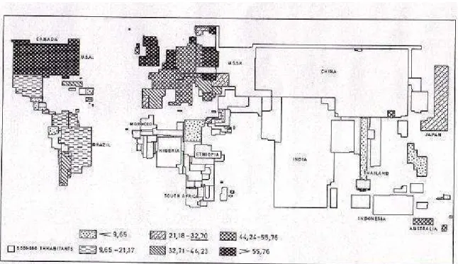
adjacency relationship, so that information from adjacent areas can be visually or mathematically integrated in an interpretive model. Therefore, a demographic cartogram is popularly used as a base map for a choropleth map. It not only symbolizes absolute numbers, but also provides more demographic information such as the size of the population at risk. Figure 3 illustrates a demographic cartogram has been used by Verhasselt and Timmermans (1987) in male cancer (due to trachea, bronchus, and lung) distribution [49]. As we noticed in Figure 3, ranked rates are subdivided into 7 classes. A question may be arisen: how to define the number of classes with the purpose of mapping a maximum amount of information. An equal class range is one of the options, but it has the risk to produce non-case class interval. An equal number of case data in each class is another option, but it has the risk to bias the areal pattern [49]. The best way is to define natural breaks as class limits. If the classification scheme is inappropriate, the distribution on the map may give a false impression [49].
Figure 2: A sample dot map (Global geocancerology 1986: lung cancer cases in Fredericia 1968-1972)
Figure 3: A sample choropleth map: Distribution of mortality in males due to cancer of the trachea, bronchus, and lung
Statistically, rates for small areas, such as census blocks, are unstable in comparison with large areas. A solution to this is to aggregate data into larger geographic areas. It is called Spatial Aggregation [37]. For rare disease such as cancer, when actual number at certain level of spatial area is small, it makes more sense to calculate and map disease rates at higher-level large scale areas. However, High-level aggregation has its trade-off, which is the loss of local-level information. Statistical tests for randomness are meaningful to evaluate the possibility of random rate difference across areas.
As stated in [37], one limitation of cholopleth maps is that they assume uniformity of features within each observed polygon even though there may be extreme variation. Also high-level aggregation will result in the loss of local-level information. For instance, suppose we have a disease cluster that includes four adjacent census-block groups. And each census block belongs to a different census tract. As we know, census tract is a high level aggregation of census block. In this case, if census tract is the baseline level of aggregation, then we will miss census-block information and lose the underlying cluster. The only solution for this is to create a smoothed rate. Creating smoothed rates starts with collecting information at lower-level of aggregation, follows with calculating rates for overlapping areas rather than non-overlapping areas. The result is a map with smoothed rates.
In disease epidemiological study, sometimes we are interested in tracing whether there is a significantly increased incidence rates in specific areas. The solution for this is probability maps. The probability map is generally applied on choropleth maps, with each polygon representing a p value. It tests whether the observed number of cases in each area is significantly greater than the expected number of cases [11].
All in all, disease mapping involves a series of options with respect to the choice of scale and base map, the number of classes, and the cancer data to be represented. The comparability of projection, scale, class intervals, colors and / or shading, size of spatial units and of population at
risk, total population and/or sex, age groups, method of standardization, and period should be taken into account.
4.0 Spatial Analysis in disease clusters
“A cluster is an excess of cases in space (a geographic cluster), in time (a temporal cluster), or in both space and time. [28]” There are two different types of clusters: one is “true cluster”; the other is “perceived cluster”. True clusters occupy less than 5% of all reported clusters. True clusters can be distinguished from perceived clusters based on following domains (refer to table 1). Table 1: True Cluster vs. Perceived Cluster [28]
Cluster type Common etiology or cause
Health outcome Potential exposure
Exposure-health link
Statistically significant True Cluster Yes Cases with
specific diagnosis or a set of symptoms related to a common exposure or etiology Common exposure Identified Yes Perceive cluster No (some due to chance) Cases of unrelated illness Common exposure is absent Unknown No
Obviously, chance can play a role in the way disease occurs in a population. However, the objective of analysis of disease clusters is to find the true clusters. According Gatrell and Bailey (1995), there are three general types of spatial analysis: visualization, exploratory data analysis and model building [17]. During most analysis, a combination of techniques will be used with the data first being displayed visually, followed by exploration of possible patterns and possible modeling.
4.0.1 Data Visualization
The first step in any data analysis is to inspect data. Visual displays of information using dot/spot maps or cholopleth maps will provide the epidemiologist with the basis for generating hypotheses. Map overlay operations allow analyst to display more than one attribute on a map at a time. Since it can visually display locations that meet specific criteria, map overlay operations are applied to look for potential carcinogenic risk factors. Besides the visual presentations, GIS can facilitate a multilayer geographic analysis [37]. For instance, suppose that we want to identify individual newborns with the greatest risk of nuclear exposure, which might be a risk factor for childhood leukemia. The birth certificates include residential address of the mother. Through overlay operations, we could link the data layer with residential address location of newborn with another layer containing the block group information. After multilayer geographic analysis, we could generate a list of names and addresses of newborns living in the census block groups with elevated risk of nuclear exposure.
Measurement allows the analysts to calculate straight-line distances between points and areas. Distance as a measure of separation in space is a key variable used in many kinds of spatial analysis. For instance, in the environmental exposure study, the distance measurement from a household to the nearest toxic dump site is critical.
Buffering is another powerful spatial analysis tool. GIS can create polygons and analyze the spatial relationships among units of observation. Buffers are particularly useful in identifying people at risk of exposure to environmental hazards.
4.0.2 Exploratory Data Analysis and Modeling
Spatial analytical methods can be divided into two categories: one is exploratory analytical techniques, which are used to describe the locational characteristics; the other is explanatory analytical techniques, which are used to analyze spatial inter-relations [38]. Exploratory data analysis aims to identify space-time clusters and to develop hypotheses. Openshaw’s geographic analysis machine (GAM: see detail below.) is an example of exploratory data analysis. Exploratory data methods are also valuable in searching areas with high prevalence rates. The probability maps, as we discussed in disease mapping section, have long used to identify statistical significance of prevalence rates. But the trade-off of this method is that it doesn’t show actual rates and population statistics. An alternative method is Empirical Bayes Smoothing, in which the smoothed rates are adjusted according to the size of the population [9, 33]. As a result, it represents a compromise between probability mapping and choropleth mapping of rates [11]. Because the rates of small areas are smoothed more than those for large areas, it conquered the small numbers problem [11].
In Modeling, specific hypotheses are formally tested or predictions are made. “In general, modeling involves the integration of GIS with standard statistical and epidemiologic methods [8]”. Spatial interaction and spatial diffusion models are of particular relevance to the infectious diseases. Spatial interaction models analyze and predict the movement of people from place to place. By accurately modeling these movement flows, it is possible to identify areas at risk for disease transmission and thus target intervention efforts [9]. Spatial diffusion models analyze and predict the spread of phenomena over space and time and have been widely used in understanding spatial diffusion of disease [9]. Modeling is more suitable to diseases with short latencies [9].
In general, GIS are useful for exploratory spatial analysis but not meaningful for confirmatory analysis [25]. In order to analyze spatial inter-relations, confirmative statistical tools and a number of epidemiological analytical techniques have been integrated into GIS in the disease clustering study. In the following sections, we will talk about statistical methods in spatial analysis, methods in space-time clustering and Data Mining in spatial analysis.
4.0.3 Explanatory Data Analysis
Statistical Methods in disease clusters
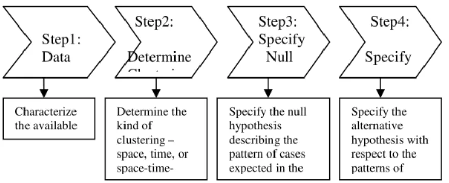
From statistical point of view, “clustering is usually considered in terms of local high rates, the occurrence of foci of particularly low local rates – negative clusters – also has aetiological significance [35].” Statistical analysis is meaningful since it has usually consisted of a significance test to identify those high rates that were likely to have occurred from influences other than random fluctuations. Based on this principle, Warterberg and Greenberg indicated four steps to define a cluster in [50] (refer to figure 3). This analytical procedure aims to evaluate how unusual the observed pattern of cases is relative to the patterns that would be expected in the hypothesis model. The objective of testing for clustering is to tackle two issues.
§ Is there a general tendency for clustering to occur and where?
Figure 3: Define a cluster
There are a number of statistical methods on the tendency analysis of clusters detection. Cuzick and Edwards categorized them into three general methodological groups: methods based on cell counts, methods on autocorrelative adjacencies of cells with high counts, and methods on distance between events [11]. Based on [35], we concluded those methods into table 2. Here we want to emphasize three commonly-used methodologies. They are nearest neighbor analysis, quadrat analysis (cell count analysis), adjacency clustering analysis and spatial autocorrelative analysis. Step2: Determine Clustering Step3: Specify Null Step1: Data Step4: Specify Characterize the available data. Determine the kind of clustering – space, time, or
space-time-Specify the null hypothesis describing the pattern of cases expected in the Specify the alternative hypothesis with respect to the patterns of
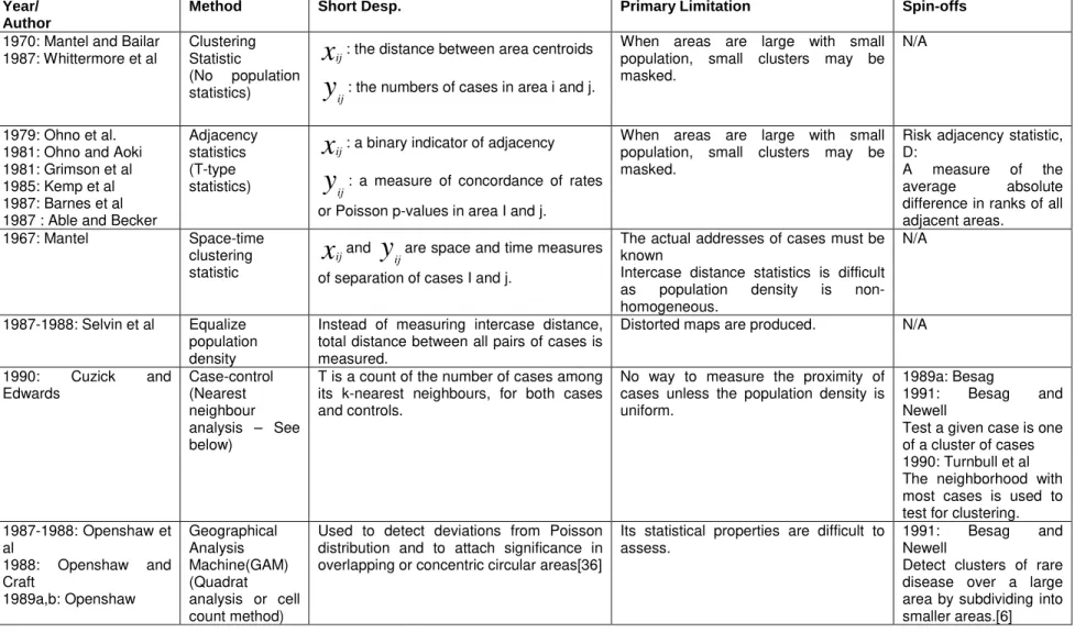
Table 2. Testing methods for a tendency to cluster Year/
Author
Method Short Desp. Primary Limitation Spin-offs
1970: Mantel and Bailar 1987: Whittermore et al
Clustering Statistic
(No population statistics)
x
ij: the distance between area centroidsy
ij: the numbers of cases in area i and j.When areas are large with small population, small clusters may be masked.
N/A
1979: Ohno et al. 1981: Ohno and Aoki 1981: Grimson et al 1985: Kemp et al 1987: Barnes et al 1987 : Able and Becker
Adjacency statistics (T-type statistics)
x
ij: a binary indicator of adjacencyy
ij: a measure of concordance of rates or Poisson p-values in area I and j.When areas are large with small population, small clusters may be masked.
Risk adjacency statistic, D:
A measure of the average absolute difference in ranks of all adjacent areas.
1967: Mantel Space-time clustering statistic
x
ijandy
ijare space and time measuresof separation of cases I and j.
The actual addresses of cases must be known
Intercase distance statistics is difficult as population density is non-homogeneous.
N/A
1987-1988: Selvin et al Equalize population density
Instead of measuring intercase distance, total distance between all pairs of cases is measured.
Distorted maps are produced. N/A
1990: Cuzick and Edwards Case-control (Nearest neighbour analysis – See below)
T is a count of the number of cases among its k-nearest neighbours, for both cases and controls.
No way to measure the proximity of cases unless the population density is uniform.
1989a: Besag
1991: Besag and Newell
Test a given case is one of a cluster of cases 1990: Turnbull et al The neighborhood with most cases is used to test for clustering. 1987-1988: Openshaw et al 1988: Openshaw and Craft 1989a,b: Openshaw Geographical Analysis Machine(GAM) (Quadrat analysis or cell count method)
Used to detect deviations from Poisson distribution and to attach significance in overlapping or concentric circular areas[36]
Its statistical properties are difficult to assess.
1991: Besag and Newell
Detect clusters of rare disease over a large area by subdividing into smaller areas.[6]
Nearest neighbor analysis is one of commonly-used methodologies in detecting point patterns. It uses inter-case distance to represent the strength of point patterns [38]. Significance tests are used to evaluate the overall tendency toward clustering. However, nearest neighbor analysis has its own problem. For instance, it fails to distinguish between homogenous and random patterns. Also different results will obtained if different size areas are analyzed with the same data [38]. In order to overwhelm its shortcomings, several alternatives to the nearest neighbor analysis have been invented and used in cancer epidemiological studies. Bithell (1990) estimated a relative-risk function for childhood leukemia in Cumbia, England [6]. Gatrell and Bailey (1996) estimated k functions for randomly selected cases and controls of childhood leukemia in Lancashire, England [17]. A common approach based on nearest neighbor analysis is developed by Cuzick and Edwards. It is called the kth nearest neighbor approach [12]. Instead of actual intercase distances, it used relative distances. The procedure of the kth nearest neighbor approach derives from a case-control paradigm - sampling non-cases from the population at risk. The statistic tests are developed based on the number of cases among the kth nearest neighbors of each case and the number of cases nearer than the k nearest control [12]. The attractive feature of this approach is that it accounts for the problem of geographic variation in population density.
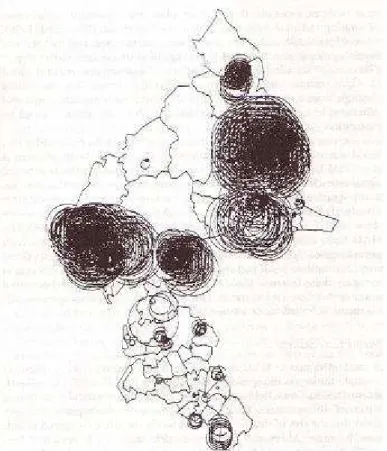
Another commonly-used methodology in detecting point patterns is quadrat analysis or cell count method. It is used to “test for complete spatial randomness” [38]. Quadrat count methods that compare observed and expected distributions of cases over a number of small areas. It tests for the presence of clustering in general. Openshaw et al. developed GAM (see figure 4 [40]), which is based on quadrat analysis, to test the significance of childhood leukemia cancer clusters. An alternative method which is based on quadrat analysis and similar to GAM is called the spatial scan statistic. Kulldorff, Feuer, Miller, et al. used the spatial scan statistic with multiple testing on the clustering study of breast cancer mortality in the northeast United States [33, 27].
Figure 4: The results of an analysis of clustering of childhood acute lymphoblastic leukemia in a study region in England using GAM.
Adjacency clustering analysis is used to evaluate the similarity of adjacent areas. The general form of adjacency clustering is:
y
x
ij i j ijT
=
wherex
ij andy
ij are measures of similarity, or separation, of observational units i and j [35].
Within this category, the Ohno method was developed to evaluate clustering of areal data on a large scale. Areas are compared with respect to concordance; adjacent areas are concordant if they have the same category and are discordant otherwise [38]. The Ohno method has its potential shortcoming: all dissimilar joins are treated alike [38]. The alternative to Ohno method is rank adjacency statistic D. Since it measures the average absolute difference in ranks of all adjacent areas, D test can be used when population density is heterogeneous. The limitation of D test is that it only applied to non-parametric data [36]. Both Ohno and D test are used to evaluate areal clustering of cancer mortality. Geary’s c and Moran’s I are two commonly used methods for areal patterns. By comparing adjacent area values, they would assess the level of large scale clustering. They have been frequently applied to examine areal clusters, including cancers [38]. Monte Carlo simulation model and hierarchical clustering structure can be used to assist adjacency analysis. Monte Carlo techniques can be used as a tool to simulate some random process whereas hierarchical clusters of high risk areas can be constructed by ranking disease rates for high-ranking units from high to low [38].
Spatial autocorrelation analysis includes a class of methods which measure spatial dependence, the association between a value at a particular location and values for nearby or adjacent areas. It is useful for finding disease clusters based on area data [11]. Glick used spatial autocorrelation analysis to analyze sex-specific cancer mortality rates among 67 counties of Pennsylvania [22] and skin cancer mortality in United States [23].
The methods we discussed so far are used to detect spatial disease clusters in one dimension. As we know, carcinogenic process is a long latency period. Hence, in cancer epidemiological study, we have to synthesize person, place, and time and consider them as three basic elements.
Space-time clustering
The detection of clusters of disease in space, time, or in both space and time is important to epidemiologist. An aggregation of cases over time and over space may provide a clue to generate causative hypotheses. “Space clustering is a non-uniform distribution of the cases over the area relative to the underlying population. Time clustering is a non-uniform distribution of the cases over the duration of the study. Space-time clustering is an interaction between the places of onset and the times of onset of the disease. [52]” In [52], Williams reviews various methods for detecting clustering in both space and time. Here we discuss some commonly-used methods used in cancer epidemiological study (See Table 3). Within above methods, Ederer’s method has been the most popular one [52]. Many these methods have been conducted on case-clustering studies of leukemia, Hodgkin’s disease or Burkitt’s lymphoma. Studies of space-time clustering on leukemia and Hodgkin’s disease have not yielded convincingly positive findings. Although there is a strong evidence for clustering of Burkitti’s lymphoma in Africa, further investigations are necessary to determine whether case-to-case transmission may take place [52]. In addition, most of common cancers show some degree of familial clustering. In cancer epidemiological study, a variety of associations with potential environmental factors and personal attributes of individuals have been demonstrated. Various statistical methods have been used to test for familial aggregation.
Table 3: Methods in Space-Time Clustering [52]
Year Author Methods/ Extension
Short Description & Primary Strength
Primary Limitation Use in Cancer Epidemiological Study 1963, 1964a 1968 Knox Pike and Smith Knox’s method
Pike and Smith’s Extension
Knox takes all possible disease cases and evaluates whether there is some positive relationship between temporal and spatial distance, between the members of a pair. Pike and Smith’s extension can handle the cases with long latent period, while Knox cannot.
1. Sensitive to space-time clustering, insensitive to purely space or time clustering. 2. Difficult to specify critical times and distance for an unidentified disease process.
1. Used in epidemiological study in Burkitt’s lymphoma study. (Doll, 1978) [14]
2. Used in detect time-space clustering in Hodgkin’s disease (Chen et al, 1984) [8] 1967 1971 Mantel Klauber Mantel’s Generalized regression method Two Sample Problem / Several Samples (Extension of Mantel’s method)
y
x
ij j i ijz
<=
wherex
ijis a spatialmeasure between points I and j and
y
ijis a temporal measure.It emphasizes the effects of large space and time difference.
Two Sample Problem method deals with the situation when two sets A and B of distinguishable cases with space coordinates and time coordinates.
Still cannot avoid the need for identifying critical times and distances.
For two sample problem, randomization experiment is recommended to perform.
1. Test for space-time clustering for childhood leukemia in San Francisco during the 20 year period.(Klauber and Mustacchi, 1970) [26]
2. Used in detect time-space clustering in Hodgkin’s disease (Chen et al, 1984) [8]
1974 Pike and Smith
Pike and Smith Case Control method
Using case-control approach to ascertain relevant contact from person to person.
Need to define critical times and distances, as well as critical control group.
Detect clustering of leukemia, Hodgkin’s disease, and other lymphoma’s in Bahrain (Hamadeh et al, 1980) [19]
1964 Ederer, Myers, and Mantel
Ederer’s Method Instead of using paired distance technique, it examines the distribution of cases within a time-space unit.
Data have to be examined to see which is occurring.
1.Test time-space clustering of leukemia cases (Ederer, Myers and Mantel, 1966) [15]
2. Used in detect time-space clustering in Hodgkin’s disease (Chen et al, 1984) [8]
1966 David and Barton
David and Barton’s Method
It applies a test for studying the randomness of points on a plane. It gave the exact mean and variance of the statistic.
A statistical weekness: multi-degree of freedom character.
It has been used in the cancer literature.
Spatial Data Mining
Statistical spatial analysis is widely used technique for analyzing spatial data [35]. Statistical analysis handles well with numerical data, and enables optimization and building models [32]. Nevertheless, it has some shortcoming such as poor dealing with symbolic data, high computational complexity and others [32]. Especially statistical analysis usually requires the assumptions regarding to statistical independence of spatial data. Such assumptions are often unrealistic since they ignored the influence of neighborhood relationship. In addition, with advancement in computerization and data collection, large and continuously growing amount of data makes it impossible to interpret all data manually. To overcome these weaknesses of statistical analysis, spatial data mining has been proposed to analyze data from large spatial database.
“Spatial data mining is the process of discovering interesting and previously unknown, but potentially useful patterns from large spatial datasets [45]”. The complexity of spatial data and intrinsic spatial relationships limits the use of conventional data mining techniques. The data inputs of spatial data mining consist of two distinct types of attributes: non-spatial attribute and spatial attribute. Spatial attributes have the following features: (1) rich data types (including extended spatial objects such as points, lines, and polygons); (2) implicit spatial relationships among the variables (including overlap, intersect, and behind); (3) observations are not independent; and (4) spatial autocorrelation among the features [44]. Quinlan (1993), Barnett & Lewis (1994), Agrawal & Srikant (1994), Jain & Dubes (1988) propose one possible way to deal with implicit spatial relationship. That is materializing the relationships into traditional data input columns first and then applying classical data mining techniques. However, it is criticized for losing information [45]. Another way, as stated in [45], is to develop models or techniques to integrate spatial information into the spatial data mining process. Here we want to cover several models in spatial data mining.
Spatial Classification Models
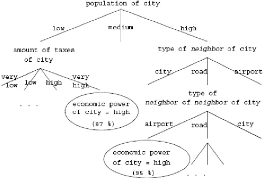
“Given a set of data (a training set) with one attribute as the dependent attribute, the classification task is to build a model to predict the unknown dependent attributes of future data based on other attributes as accurately as possible [44]”. Decision Tree Approaches is proposed in [17]. It employs neighborhood relationship and considers not only attributes of the classified object, but also the attribute values of neighboring objects. Objects are considered neighbors if they satisfy some neighborhood relations such as overlap close-to, etc. Figure 5 depicts a sample decision tree. The limitation of this approach is that it doesn’t take into account spatial autocorrelation [44]. Logistic Regression Modeling is a classical classification approach. The fundamental limitation of this approach is that it assumes that the sample observations are independently generated. It ignores spatial data property: observations are not independent. Spatial Autoregression model (SAR) introduces a parameter
ρ
which reflects the strength of spatial dependencies between the elements of the dependent variables. Whenρ
= 0, it collapses to the logistic regression model [43, 45]. The benefits of SAR in comparison with logistic regression model are: (1) the residual error will have much lower spatial autocorrelation, i.e., systematic variation. (2) If the spatial autocorrelation coefficient is statistically significant, then SAR will quantify the presence of spatial autocorrelation. (3) SAR will have a better fit, i.e., a higher R-squared statistic [43, 44]. Another model used for spatial autocorrelation is called Markov Random Fields (MRFs). It generalizes Markov chains to multi-dimensional structures. It has been applied in image processing and spatial statistics, where they have been used to estimate spatially varying quantities [44].Figure 5: A sample decision tree
Detecting Spatial Outliers
Spatial outliers are observations that are inconsistent with those in their neighborhood. The identification of spatial outliers can lead to the discovery of unexpected knowledge. It has a number of practical applications in the fields of transportation, epidemiology, precision agriculture, weather prediction, etc [44]. Spatial outlier detection approaches can be classified into three categories: set-based outliers, multi-dimensional space-based outliers, and graph-based outliers. A set-based outlier is a data object whose attributes are inconsistent with attribute values of other objects in a given data set regardless of spatial relationships while both multi-dimensional space-based outliers and graph-space-based outliers are space-based on spatial relationships. However, spatial outlier detection is challenging to perform since (1) the choice of a neighborhood is critical. (2) statistical tests for spatial outliers have to consider not only the distribution of the attribute values at various locations but also the distribution of aggregation function of attribute values over the neighborhoods. (3) the computational cost of determining parameters for a neighborhood-based test can be high [44].
Spatial Co-location Rules
Spatial co-location rules are a generalization of association rules to spatial datasets. Conventional association rules are widely used in finding items frequently bought together in market basket study. On a map, there are a number of variables collected to define a specific location. A set of events, i.e. Boolean spatial features define and identify different variables.
Co-location patterns represent frequent co-occurrences of a subset of Boolean spatial features [43]. (Refer to Figure 5 [45])
Figure 5: (a) Illustration of Point Spatial Co-location Patterns. Shapes represent different spatial feature types. Spatial features in sets {‘+’, ‘x’} and {‘o’, ‘*’} tend to be located together. (b) Illustrate of Line String Co-location Patterns. Highways, e.g.: Hwy100, and frontage roads, e.g., Normandale Road, are co-located.
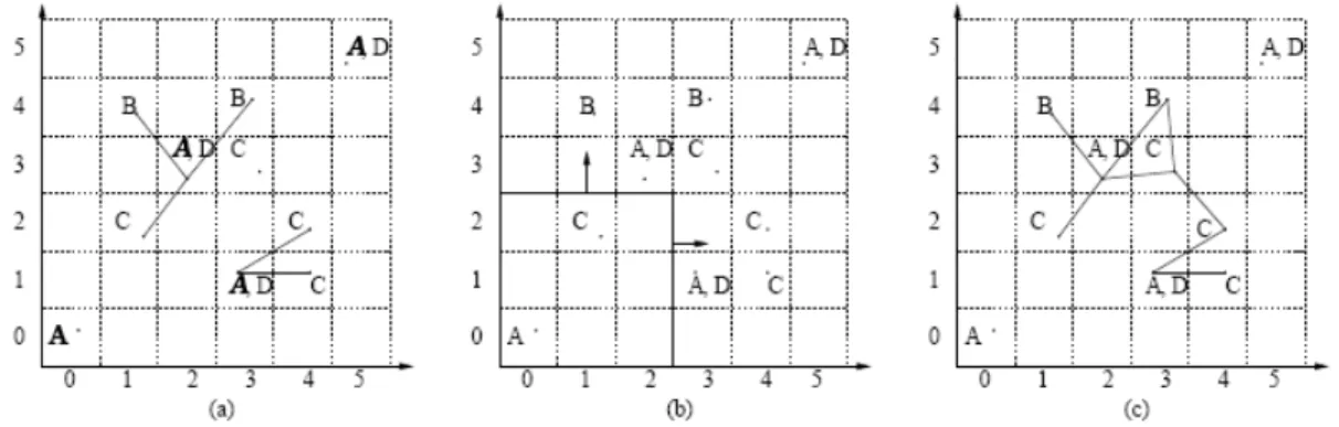
There are three different models to detect spatial co-location patterns. The reference feature centric model is focusing on a specific Boolean spatial feature. The interest of this model is to find the co-locations of other relevant features to the reference feature [44]. The window centric model focuses on land-parcels. The interest of this model is to discover some other features in a given land parcel [44]. The event centric model, its interest is to find subsets of spatial features to occur in a neighborhood [44]. Refer to Figure 6 [44] to tell the differences of these three models.
Figure 6: (a) Reference feature centric model. The instances of A are connected with their neighboring instances of B and C by edges. (b) Window centric model. Each 3X3 window corresponding to a transaction. (c) Event centric model. Neighboring instances are joined by edges.
Spatial Clustering
Spatial clustering is a process of grouping a set of spatial objects into clusters so that objects within a cluster have high similarity, but are dissimilar to objects in other clusters [44]. Spatial
clustering focuses on discovering hot spots, where there are unusual dense event clusters across time and space.
There are three distinguished types of clusters [45]. Complete spatial randomness cluster, its distribution patterns are random. Spatial objects within this cluster are independent with each other. Spatial clusters and declusters are two different non-random patterns. Spatial clusters are aggregated patterns whereas declusters are uniformly spaced patterns.
Statistical methods are applied to test significance of spatial clusters and to quantify deviation of patterns. One type of statistics is based on quadrats i.e. well defined areas; the other type of statistics is based on distances (Ripley’s K-function) [45].
Knowledge Discovery in Database
Knowledge discovery in database (KDD) is a non-trivial exaction process of discovering implicit, unknown, and potentially useful patterns from database [16]. The process of KDD involves data selection, data reduction, data mining and the evaluation of the data mining results. The core of the process is data mining, which consists of data analysis and discovery algorithm [16]. There are a wide variety of algorithms used in KDD. The objectives of these algorithms are to fulfill the following generic tasks [17]:
§ Class identification: grouping the objects of the database into meaningful subclasses
§ Classification: finding rules that describe the partition of the database into a given set of classes
§ Dependency analysis: finding rules to predict the value of some attribute based on the value of another attribute
§ Deviation detection: discovering deviations from the expectations such as outliers in a class of object.
According to the features of spatial data, spatial database system is defined as relational database plus a concept of spatial location and spatial extension. The explicit location and spatial extension form implicit relation of spatial neighborhood [17]. And most KDD algorithms for spatial databases will make use of neighborhood relationships, in which the attributes of neighbor objects may have an influence on the observed object [17]. Thus, the basic framework for spatial data mining is based on the concepts of neighborhood graphs and neighborhood paths which are defined with respect to neighborhood relations between objects [16]. Spatial data mining serves as an analysis process in KDD for four main tasks: spatial clustering, spatial characterization, spatial trend detection and spatial classification.
In [32], Koperski and Han (1996) investigated and implemented a number of algorithms which are based on knowledge discovery techniques for large databases. The study is focused on mining strong spatial association rules in geographic information databases. In the first stage-attribute-oriented induction, knowledge is summarized in a form of relationships between spatial and non-spatial attributes at generalized high concept level. Combination of attribute-oriented induction with clustering analysis provides a possibility of describing spatial behavior of similar objects or to determine characteristics of distinct clusters. At the end, spatial association rule is applied to indicate certain strong association between a set of spatial and non-spatial predicates. As a closing statement, Koperski and Han points out that discovery of spatial association rules is a new and promising direction in spatial data mining.
Forgionne, et al (2000), in [18], introduces a prototype of Cancer Surveillance System (CSS). CSS consists of a geographical information system (GIS), an executive information system (EIS), and a decision support system (DSS). The prototype GIS is used to extract data, create thematic maps and provide inputs for the EIS. EIS will provide a database management system (DBMS) and an intelligent decision support system processor (IHP). DBMS will store all the spatial and non-spatial data into data warehouse. The IHP captures the DBMS’s data, updates the DSS’s
spatial and temporal statistical models, performs DSS analyses and evaluations, and generates detailed reports of the results. Data mining techniques will be employed to extract cancer patterns from the data. Descriptive modeling or predictive modeling will be involved in the process of spatial data mining analysis. Descriptive modeling serves as an exploratory tool in discover previously unknown patterns, trends, and associations in the data. Predictive modeling allows testing specific hypotheses. Certain artificial intelligence technologies, such as neural networks and genetic algorithms, and statistical methodologies will assist spatial data mining analysis. As a whole, this DSS will be available to deliver the methods, techniques, and developed models to the interested domains (cancer care, cancer surveillance, and cancer prevention).
4.1 Cluster Analysis Software
In [5], Anselin (2004) reviews four free software packages that can be used in a spatial analysis of cancer clusters: CrimeStat, GeoDa, SaTScan, and packages developed in the open source R programming environment. The software are evaluated with respect to their abilities to answer the following questions:
§ Given a data set, where are the potential cancer clusters?
§ Given that there may be a cluster, what is its statistical significance?
§ Given a suspect location, is there a cluster found around it?
These four software have been developed to implement methods for spatial data analysis. Hence, these cluster analysis software should have an efficient interface to the GIS which can provide a connection. With two-way connection, GIS can input the extracted data to cluster analysis software whereas the software can feed back results for map display. In addition, a software tool for cancer clusters analysis should take into consideration these essential requirements:
1. Effective data input: spatial data features (stated in spatial data mining section), cancer data features (stated in using cancer data in GIS section);
2. Spatial information: distance measurements
3. Descriptive statistics: identification of extreme high or low disease incidence, outlier detection, smoothing rates.
4. Point pattern analysis: distance or quadrat based statistics to identify the clusters and test the null hypotheses.
5. Spatial autocorrelation analysis: measures of global and local spatial autocorrelation and to identify areas with elevated risk with similar area surrounded, or to identify spatial outliers
6. Visualization of the results: maps and / or graphs indicating outliers and significant clusters.
7. Program output: an effective interface to the GIS to present output on maps.
In general, none of above free software satisfies all these criteria. And also there is no single commercial alternative that meets all these criteria. For details, please refer to Appendix for features of four free software [5].
4.2 Discussion
Up till now, we did an extensive methodological review on spatial analysis. We followed this backbone: start with simple data collection (using cancer data in GIS), follow by complex disease mapping and then more complicated spatial analysis for detecting disease clusters. In spatial analysis, we cover commonly-used methodologies in both exploratory data analysis and explanatory data analysis. Now it is useful to outline some of the main issues in the analysis of cancer clusters in order to put all above methodologies into right position in the procedure of analysis.
The first issue to consider in the analysis of cancer clusters is the type of spatial data to be analyzed. There is an important difference between point data and areal data. Data on individual events such as the exact addresses of patients represents as points. Aggregated data such as a count of events or a rate are treated as areal data. As we mentioned before, because of individual case data restriction and privacy protection, some cancer information may not contain actual address information, but instead have information at larger, or aggregate, geographical areas, such as block groups, census tracts, districts, or counties. In this case, areal data are commonly-used in analysis of cancer clusters.
The second issue to consider in the analysis of cancer clusters is the type of analysis. For areal data, a cluster refers that an areal unit is surrounded by other similar areas. In other words, the analysis focuses on finding an area with high risk which is surrounded by other similar areas with high risk, rather than by chance. There is another situation where an area with higher risk than other neighboring areas. We call it as spatial outlier. Both cluster and outlier are non-random. Spatial randomness means uniform distribution or points could be anywhere with equal probability. Usually spatial randomness needs to be specified in null hypothesis. The observed values will be tested for compatibility against this null hypothesis.
The third issue to consider in the analysis of cancer clusters is heterogeneity of area size and population. For instance, when the risk is estimated for areal data for small area or with different population, the precision of the estimate is affected. Case-control approach could overcome this shortcoming by comparing the observed pattern to control group. Another alternative is to smooth the observed rates.
The fourth issue to consider in the analysis of cancer clusters is to distinguish global tests and local tests. Global tests are designed to test against the null hypothesis of spatial randomness for the data set as a whole. The objective is to find significant patterns. In contrast, local tests are designed to identify the locations of clusters or spatial outliers. Among local tests, focused tests aim to find the causative clusters. For instance, clusters of cancer around a source of carcinogens. Inter-case distances and quadrat cell counts are two basic methods for point data. The distances or the density of points in a quadrat area are compared to the null hypothesis of spatial randomness. Significant tests are performed to indicate the true clusters. We indicated some major statistical methods which belong to this category, such as nearest neighbor analysis, GAM, etc. For areal data, cluster tests can be classified into two broad types. First, the centroid of an area can be represented by a point and all events within this area unit are associated with this point. Quadrat analysis can be applied to collect individual points. Spatial scan statistics is one of them. Alternatively, areal clusters can be detected from spatial autocorrelation analysis and adjacency analysis. They consist of evaluation of adjacency similarity and attribute similarity. However, the difficulty of these two methods is how to properly define neighbor areas.
The fifth issue to consider in the analysis of cancer clusters is long latency of carcinogenic process. It is not enough to detect cancer clusters in one dimension. Spatial-time clustering analysis is proposed to detect clusters of disease in space, time, or in both space and time. An aggregation of cases over time and over space may provide a clue to generate causative hypotheses.
All statistical analysis handles well with numerical data, and enables optimization and building models. Nevertheless, it has some shortcoming such as poor dealing with symbolic data, high computational complexity and others. Especially statistical analysis usually requires the assumptions regarding to statistical independence of spatial data. Such assumptions are often unrealistic since they ignored the influence of neighborhood relationship. The sixth issue to consider in the analysis of cancer clusters is to overcome those weaknesses of statistical analysis. The solution is spatial data mining. It provides a flexible way to integrate all spatial data and non-spatial data into data mining process. It can develop models or techniques to perform non-spatial autocorrelation analysis, spatial randomness tests, and spatial co-location (spatial association) tests in order to discover spatial clusters or spatial outliers. Several knowledge discovery systems
have been designed using spatial data mining as a core component. The results show that spatial data mining is a new, promising way to detect clusters. There are not much studies of using spatial data mining on detecting disease clusters. In addition, there is no software has been developed using spatial data mining to detect disease clusters. We believe using spatial data mining in detecting disease clusters would be a ‘’hot” research spot in the near future.
Bibliography
1. Adami, H., Trichopoulos, D., (2002) “Concepts in Cancer Epidemiology and Etiology”. Adami, H., Hunter, D., Trichopoulos, D., (ed) 2002. Textbook of Cancer Epidemiology, Oxford University Press, New York, pp. 87-112.
2. Albert, D.P., Gesler, W.M., Wittie, P.S., 1995. “Geographic Information System and Health: An Educational Resource”. In Journal of Geography, 94(2), pp. 350-356.
3. Alexander, F.E., Ricketts, T.J., Williams, J., and Cartwright, R.A., 1991. “Methods of mapping and identifying small clusters of rare diseases with applications to geographical epidemiology”. In Geographical Analysis, 23(2), pp.158-173.
4. Akhtar. R., 1982. The Geography of Health: an Essay and a Bibliography, Marwah Publications, New Delhi.
5. Anselin, L, 2004. “Review of Cluster Analysis Software”. Report in Fulfillment of Consultant Agreement #2003-04-01with The North American Association of Central Cancer Registries, Inc. http://www.schs.state.nc.us/NAACCR-GIS/pdfs/clustersoftwareFinal.pdf
6. Besag, J., Newell, J., 1991. “The detection of clusters in rare diseases”. In J.R. Stat. Soc. 154: pp. 143-55.
7. Bithell J.F., 1990. “An application of density estimate in geographical epidemiology”. In Stat. Med 1990; 9: pp. 691-701.
8. Chen, R., Mantel, N., Klingberg, MA., 1984. “A study of three techniques for time-space clusterings in Hodgkin’s Disease”. In Stat. Med, 3: pp. 173-184.
9. Clarke, K.C., McLafferty, S.L., Tempalski, B.J., 1996. “On Epidemiology and Geographic Information Systems: A Review and Discussion of Future Directions” in Emerging Infectious Diseases, 2(2), pp. 85-92.
10. Clemmesen J., 1986. In: Howe GM(ed) Global geocancerology. A world geography of human cancers.Churchill Livingstone, Edinburgh, pp 191-198.
11. Cromley, EK, McLafferty, SL, 2002. GIS and Public Health. The Guilford Press, New York, London: pp.130-157.
12. Cuzick, J., Edwards, R., 1990. “Spatial Clustering for inhomogeneous populations”. In J R Stat Soc 1990; 52: pp. 73-104.
13. Doll, R., 1978. “An epidemiological perspective of the biology of cancer”. In Cancer Research, 38: pp. 3573-3583.
14. Dunn, C.E., 1992. ”GIS and Epidemiology (Education, Training, and Research Publication 5)”. The association for Geographic Information, London.
15. Ederer, F., Myers, M.H., and Mantel, N., “A statistical problem in space and time: do leukemia cases come in clusters?” in Biometrics, 20: pp.626-638.
16. Ester M., Kriegel, HP, Sander, J., 2001. “Algorithms and applications for spatial data mining”. In Geographic Data Mining and Knowledge Discovery, Research Monographs in GIS, Taylor and Francis: pp. 1-32.
17. Ester M., Kriegel, HP, Sander, J., 1997. “Spatial Data Mining: A Database Approach”. In Proc. Of theFifth Int. Symposium on Large Spatial Databases, Berlin, Germany.
18. Forgionne, G, Gangopadhyay, A, Adya, M., 2000. “Cancer Surveillance Using Data Warehouse, Data Mining, and Decision Support Systems”. In Top Health Inf Manage Aug. 21, 2000. 21(1): pp.21-34.
19. Gasler SL, Bailey, TC, 1996. “Interactive spatial data analysis in medical geography”. In Soc. Sci. Med. 1996; 42: pp. 843-55.
20. Gatrell, A., Senior, M., 1999. “Health and health care applications.” In Longley, P.A., Maguire, D.J., Goodchild, M.F., et al. (eds), Geographical Information Systems: Principle and Applications, 2nd Edition. Longman, London.
21. Gesler, Wil, 1986. “The uses of spatial analysis in medical geography: a review”. In Sco. Sci. Med. 23(10), 963-73.
22. Glick, B., 1979. “The spatial autocorrelation of cancer mortality”. In Soc. Sci. Med. 13D: pp. 123-130.
23. Glick, B., 1982. “The spatial organization of cancer mortality”. In Ann. Ass. Am. Geogr. 72: pp. 471-481.
24. Hamadeh, R.R., Armenian, H.K., Zurayk, H.C., 1980. “A study of clustering of cases of leukemia, Hodgkin’s disease and other lymphoma’s in Bahrain”. In Tropical and Geographic Medicine, 33: pp. 42-48.
25. Higgs, G., Gould, M., 2001. “Is there a role for GIS in the ‘new NHS’?” In Health & Place 7, 247-259.
26. Howe, G.M., 1989. “Historical Evolution of Disease Mapping in General and Specifically of Cancer Mapping”, Boyle, P., Muir, C.S., and Grundmann (Eds), Recent Results in Cancer Research: Cancer Mapping, Springer-Verlag, pp. 1-21.
27. Hjalmars, U., Kulldorff, M., Gustafsson, G, et al. 1996. “Childhood leukemia in Sweden: using GIS and a spatial scan statistic for cluster detection”. In Stat Med 1996; 15: pp 707-15. 28. Jacquez, G.M., Waller, L.A., et al. 1996. “The Analysis of Disease Clusters Part I : State of
Art”. Infect Control Hosp Epidemiol, 17: pp. 319-27.
29. Jones, K., Moon, G., 1991A. “Progress report: Medical geography”, in Progress in Human Geography, Vol. 15, pp. 437-443.
30. Kennedy, S., 1990. “The small number of problem and the accuracy of spatial databases”, Goodchild, M., Gopal, S. (Eds), Accuracy of Spatial Databases, Taylor and Francis: London, pp. 187-196.
31. Klauber, MR., Mustacch, P., 1970. “Space-time clustering of childhood leukemia in San Francisco”. In Cancer Research, 30: pp. 1969-1973.
32. Koperski, K., Han, J., 1996. “Data mining methods for the analysis of large geographic databases.” Proc. 10th Annual Conf. on GIS. Vancouver, Canada, March 1996.
http://citeseer.ist.psu.edu/koperski96data.html
33. Kulldorff, M., Feuer, EJ, Miller BA, et al, 1997. “Breast cancer clusters in the northeast United States: a geographic analysis”. In Am J. Epidemiol. 1997; 146: pp. 161-70.
34. Lam, Nina Siu-Ngan, 1986. “Geographical patterns of cancer mortality in China”. In Soc. Sci. Med. 23(3), 241-247.
35. Marshall R.J., 1991. “A review of methods for the statistical analysis of spatial patterns of disease”. In J.R. Statist. Soc. A (1991); 154, part 3: pp. 421-441.
36. Mayer, J.D., 1983. “The role of spatial analysis and geographic data in the detection of causation” in Soc. Sci. Med. 17(16), pp. 1213-1221.
37. Melnick, AL, 2002. “GIS Data Transformation: Making Maps”. In Introduction to Geographic Information Systems In Public Health. Aspen Public Inc. Gaitherburge, Maryland: pp. 45-63. 38. Moore, D.A., Carpenter, T.E., “Spatial Analysis methods and Geographic Information
Systems: Use in Health Research and Epidemiology”, 1999. in Epidemiologic Reviews. 21(2), pp. 143-161.
39. Murray, M.A., 1974. “The geography of chronic diseases”. In J.M. Hunter (ed.), The Geography of Health and Disease, University of North Carolina, Chapel Hill, 1974. pp. 101-127
40. Openshaw, S., Craft, A.W., Charlton, M., Birth, J.M., 1996. Investigation of Leukemia clusters by use of a geographical analysis machine. The Lancet, February 6, 272-273.
41. Pfeiffer, DU, 1996. “Issues related to handeling of spatial data”. In J.McKenzie (ed) Proceedings of the epidemiology and state veterinary programmes, New Zealand Veterinary Association/Australian Veterinary Association Second Pan Pacific Veterinary Conference, Christchurch, 23-28 June 1996: pp.83-105.
42. Richards, T.B., Croner, C.M., Rushton, G., 1999 “Geographic Information Systems and Public Health: Mapping the Future”. In Public Health Report. 114 (1999C). pp. 359-373. 43. Selvin, S., Merrill, D., et al. 1988. “Transformations of Maps to Investigate Clusters of
44. Shekhar, S., Huang, Y., Wu, W., Lu, CT, and et al. 2003 “What’s spatial about spatial data mining: three case studies”. In Kargupta, H., Joshi, A., (ed) Data Mining: Next Generation Challenges and Future Directions, AAAI/MIT Press: Chapter 1.
45. Shekhar, S., Zhang, P., Huang, Y., et al. 2003 “Trends in Spatial Data Mining”. In Kargupta, H., Joshi, A., (ed) Data Mining: Next Generation Challenges and Future Directions, AAAI/MIT Press: Chapter 3.
46. Teppo, Lyly, “Problems and Possibilities in the Use of Cancer Data by GIS – Experience in Finland”, Ian Masser and Francois Salge (ed), GIS and Health (GISDATA 6), Chapter 12 47. Todd, P., Bundred, P., Brown, P., 1994. “The demography of demand for oncology services:
a health care planning GIS application”. AGI ’94 Birmingham, association for Geographic Information, London, 17. 1-8
48. Verhasselt, Yola, 1993. “Geography of health: some trends and perspectives”. In Soc. Sci. Med. 30(2) 119-123.
49. Verhasselt, Y., 1989. “Problems of Cancer Mapping”, Boyle, P., Muir, C.S., and Grundmann (Eds), Recent Results in Cancer Research: Cancer Mapping, Springer-Verlag, pp. 22-27. 50. Verhasselt, Y., Timmermans A., 1987. World maps of cancer mortality. Geografisch Instuut
VUB, Brussles.
51. Wartenberg D, Greenberg M., 1993. “Solving the cluster puzzle: clues to follow and pitfalls to avoid.”in Stat Med 1993; 12: pp. 1763-1770.
52. Williams, G., 1984. “Time-Space Clustering of Disease”. In Cornell, R. (ed) Statistical Methods for Cancer Studie, Marcell Dekker, New York: pp. 167-227.

![Table 1: True Cluster vs. Perceived Cluster [28]](https://thumb-eu.123doks.com/thumbv2/123doknet/14181224.476302/11.918.126.796.312.543/table-true-cluster-vs-perceived-cluster.webp)
![Table 3: Methods in Space-Time Clustering [52]](https://thumb-eu.123doks.com/thumbv2/123doknet/14181224.476302/17.1188.196.1067.159.777/table-methods-in-space-time-clustering.webp)