Publisher’s version / Version de l'éditeur:
Proceedings of the IEEE 2012 World Congress on Computational Intelligence,
IEEE 2012 International Joint Conference on Neural Networks, pp. 1-8,
2012-06-15
READ THESE TERMS AND CONDITIONS CAREFULLY BEFORE USING THIS WEBSITE. https://nrc-publications.canada.ca/eng/copyright
Vous avez des questions? Nous pouvons vous aider. Pour communiquer directement avec un auteur, consultez la première page de la revue dans laquelle son article a été publié afin de trouver ses coordonnées. Si vous n’arrivez pas à les repérer, communiquez avec nous à [email protected].
Questions? Contact the NRC Publications Archive team at
[email protected]. If you wish to email the authors directly, please see the first page of the publication for their contact information.
NRC Publications Archive
Archives des publications du CNRC
This publication could be one of several versions: author’s original, accepted manuscript or the publisher’s version. / La version de cette publication peut être l’une des suivantes : la version prépublication de l’auteur, la version acceptée du manuscrit ou la version de l’éditeur.
For the publisher’s version, please access the DOI link below./ Pour consulter la version de l’éditeur, utilisez le lien DOI ci-dessous.
https://doi.org/10.1109/IJCNN.2012.6252624
Access and use of this website and the material on it are subject to the Terms and Conditions set forth at
Towards conservative helicopter loads prediction using computational
intelligence techniques
Valdes, Julio J.; Cheung, Catherine; Li, Matthew
https://publications-cnrc.canada.ca/fra/droits
L’accès à ce site Web et l’utilisation de son contenu sont assujettis aux conditions présentées dans le site LISEZ CES CONDITIONS ATTENTIVEMENT AVANT D’UTILISER CE SITE WEB.
NRC Publications Record / Notice d'Archives des publications de CNRC:
https://nrc-publications.canada.ca/eng/view/object/?id=10db696b-8a8c-4547-b93c-48837b7cb311 https://publications-cnrc.canada.ca/fra/voir/objet/?id=10db696b-8a8c-4547-b93c-48837b7cb311Towards conservative helicopter loads prediction
using computational intelligence techniques
Julio J. Valdes
National Research Council Canada Institute for Information Technology
Ottawa, Canada
Email: [email protected]
Catherine Cheung
National Research Council Canada Institute for Aerospace Research
Ottawa, Canada
Email: [email protected]
Matthew Li
National Research Council Canada Institute for Aerospace Research
Ottawa, Canada
Email: [email protected]
Abstract—Airframe structural integrity assessment is a major activity for all helicopter operators. The accurate estimation of component loads is an important element in life cycle manage-ment and life extension efforts. This paper explores continued efforts to utilize a wide variety of computational intelligence techniques to estimate some of these helicopter dynamic loads. Estimates for two main rotor sensors (main rotor normal bending and pushrod axial load) on the Australian Black Hawk helicopter were generated from an input set that consisted of thirty standard flight state and control system parameters. These estimates were produced for two flight conditions: full speed forward level flight and left rolling pullout at 1.5g. Two sampling schemes were attempted, specifically k-leaders sampling and a biased sampling scheme. Ensembles were constructed from the top performing models that used conjugate gradient, Levenberg-Marquardt (LM), extreme learning machines, and particle swarm optimization (PSO) as the learning method. Hybrid and memetic approaches combining the deterministic optimization and evolu-tionary computation techniques were also explored. The results of this work show that using a biased sampling scheme significantly improved the predictions, particularly at the peak values of the target signal. Hybrid models using PSO and LM learning provided accurate and correlated predictions for the main rotor loads in both flight conditions.
I. INTRODUCTION
The accurate estimation of component loads in a helicopter is an important goal for life cycle management and life extension efforts. Helicopter operational loads are complex due to the dynamic rotating components operating at high frequen-cies. Many of the problems faced by helicopter operators in terms of structural integrity are similar to those of fixed-wing aircraft: they require fatigue and damage tolerance analyses, they need to set inspection intervals consistent with the in-spection techniques available, they need to assess the effects of corrosion and other environmental degradation effects, and they also need to assess the effects of usage changes. All of these tests and analyses rely on accurate load spectra.
The development of reliable load spectra for helicopters, however, is still not mature. While direct measurement of these loads is possible, these measurement methods are costly and difficult to maintain. An accurate and robust process to estimate these loads indirectly would be a practical alternative
This work was supported in part by Defence Research and Development Canada (13pt). Access to the data was granted by Australia’s Defence Science and Technology Organisation.
to determine and track the condition of helicopter fleets. Load estimation methods can make use of existing aircraft sensors, such as standard flight state and control system param-eters, to minimize the requirement for additional sensors and consequently the high costs associated with instrumentation installation, maintenance and monitoring.
There have been a number of attempts at estimating these loads on the helicopter indirectly with varying degrees of suc-cess. Preliminary work exploring the use of various computa-tional intelligence techniques to assist in estimating helicopter loads showed that reasonably accurate and correlated predic-tions for the main rotor normal bending could be obtained for the flight condition forward level flight at full speed using only a reduced set of flight state and control system parameters [1], [2]. However, the main weakness of these previous efforts has been the tendency to underpredict the target signal. Since these predictions could be used for calculating component retirement times, an underpredicted value would indicate a less severe loading and pose a potentially large safety risk. While an overpredicted signal would provide a conservative estimate for the component’s remaining life, an overly conservative estimate is also undesirable; however, for load prediction to be useful and accepted, demonstrating slight overprediction is preferable to ensure that the impact of the actual load cycles is captured by the prediction.
Fig. 1. Australian Army Black Hawk
This paper describes continued efforts to expand the scope and improve the predictions by using different sampling meth-ods to create the training and testing sets (k-leaders and bias-ing) as well as ensemble models created from a larger suite of computational intelligence methods such as conjugate gradient
neural networks, Levenberg-Marquardt neural networks, ex-treme learning machines, and evolutionary algorithms (particle swarm optimization). The specific problem was to estimate two main rotor loads on the Australian Army Black Hawk helicopter (shown in Figure 1) using only flight state and control system (FSCS) variables during two different flight conditions. The objectives of this work were as follows: i) to extend the scope and complexity of the predictions to include more target parameters and flight conditions, ii) to compare the results obtained by the reduced subset with the full suite of input parameters, iii) to compare different sampling techniques for creating the training and testing sets, and iv) to examine the behavior of various computational intelligence techniques in building models used on their own or as hybrids.
This paper is organized as follows: Section II describes the test data, Section III explains the methodology that was followed, Section IV details the computational intelligence techniques used for search and modeling, Section V provides the experimental settings, Section VI highlights the key results and Section VII presents the conclusions.
II. BLACKHAWK FLIGHT LOADS SURVEY DATA
The data used for this work were obtained from a S-70A-9 Australian Army Black Hawk flight loads survey conducted in 2000 [3]. During these flight trials, 65 hours of flight test data were collected from a single helicopter for a number of different steady state and transient flight conditions for several altitudes and aircraft configurations. Instrumentation on the aircraft included 321 strain gauges, with 249 gauges on the airframe and 72 gauges on dynamic components. Accelerometers were installed at several locations on the aircraft and other sensors captured FSCS parameters.
One of the goals of this research was to determine if the dynamic loads on the helicopter could be accurately predicted solely from the FSCS parameters, as these parameters are already recorded by the flight data recorder found on most helicopters. The Black Hawk helicopter had thirty such FSCS parameters recorded during the flight loads survey. Two main rotor (MR) measurements were selected as targets: the main rotor normal bending (MRNBX) and the axial load on the main rotor pushrod (MRPR1). From over 50 flight conditions, two were selected for inclusion in this study: forward level flight at full speed and rolling left pullout at1.5g. While forward level flight is a steady state manoeuvre that should be relatively straightforward to predict since the parameter values remain steady through the manoeuvre, the rolling pullout manoeuvre is a more severe and dynamic flight condition that should present a greater challenge since there is much more variation in the parameter values through each recording.
III. METHODOLOGY
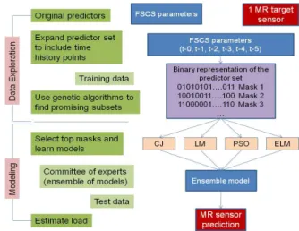
The overall goal of this work was to develop models to gen-erate accurate predictions for helicopter loads using FSCS pa-rameters. The methodology adopted for this work is illustrated in Figure 2. The application of computational intelligence and machine learning techniques to develop these models
Fig. 2. Experimental methodology
occurred in two phases: i) data exploration: characterization of the internal structure of the data and assessment of the information content of the predictor variables and their relation to the predicted (dependent) variables; and ii) modeling: build models relating the dependent and the predictor variables.
For the data exploration stage, phase space methods and residual variance analysis (or Gamma test as described in Section III-A) were used to explore the time dependencies within the FSCS parameters and the target sensor variables, identifying how far into the past the events within the system influenced present and future values. This analysis found that 5 time lags were necessary and therefore the predictor set consisted of the 30 FSCS parameters and their 5 time lags for a total of 180 predictors [1], [2]. The Gamma test then steered the evolutionary process used for data exploration. Multi-objective genetic algorithms (MOGA) were used for searching the input space to discover irrelevant and/or noisy information and identify much simpler well-behaved subsets to use as input for modeling. These subsets were found through simultaneous optimization of residual variance, gradient, and the number of predictor variables. The most promising subsets were then selected and used as a base for model search in the modeling stage. The data exploration stage that was followed in this work is described in detail in [1], [2].
During the modeling stage, a number of computational techniques were used to build models relating the target variable to the subset of predictor variables (as identified in the data exploration stage). These techniques included determin-istic optimization methods using conjugate gradient (CJ) and Levenberg-Marquardt (LM) neural networks, extreme learning machines (ELM), and particle swarm optimization (PSO) from the family of evolutionary computation techniques.
A. Gamma test (residual variance analysis)
The Gamma test is an algorithm developed by [4], [5], [6] as a tool to aid in the construction of data-driven models of smooth systems. It is a technique aimed at estimating the level of noise (its variance) present in a dataset. Noise is
understood as any source of variation in the output (target) variable that cannot be explained by a smooth transformation (model) relating the output with the input (predictor) variables. The fundamental information provided by this estimate is whether it is hopeful or hopeless to find (fit) a smooth model to the data. Since model search is a costly time-consuming data-mining operation, knowing beforehand that the information provided by the input variables is not enough to build a smooth model would be very helpful. If for a given dataset, the gamma estimates are small, it means that a smooth deterministic dependency can be expected.
Let us assume that a target variable y is related to the predictor variables x by an expression of the form y = f(x) + r where f is a smooth function and r is a random variable representing noise or unexplained variation. Under some assumptions, the Gamma test produces an estimate of the variance of the residual term using only the available (training) data. A normalized version of the variance, called the vRatio (or Vr), allows the comparison of noise levels associated with
different physical variables expressed in different units across different datasets. Another important magnitude associated with the Gamma test is the so-called gradient, G, which provides a measure of the complexity of the system.
The Gamma test is used in many ways when exploring the data. In the present case, it was used for determining how many time lags were relevant for predicting the future target sensor values, for finding the appropriate number of neighbours for the computation of Vrand G, and most importantly, for
deter-mining the subset of lagged FSCS variables with the largest prediction potential (therefore the best candidates for building predictive models). In this sense, a comprehensive exploration of the datasets for different target sensors under different flight conditions was made using Gamma test techniques in order to find subsets of the lagged FSCS variables simultaneously with minimal Vr (large prediction power), minimal G (low
complexity) and small in size (cardinality, denoted by #), thus involving a small number of predictor variables. In order to accomplish this task, a multi-objective framework using genetic algorithms was used with <Vr, G, #>as objectives.
B. Construction of the Training and Testing sets
The training/testing sets used for learning the neural net-work parameters and for independent evaluation of their performance should come from the same statistical population in order to properly assess the generalization capability of the network models learnt. Typically the entire data collection is partitioned into training/testing proportions such as 50%/50%, 75%/25%, 80%/20% or 90%/10%.
In this case, in order to work with relatively smaller training sets while keeping the representativity of its elements, clus-tering algorithms were used. The elements of the training sets were constructed by aggregating the vectors representing the different classes constructed by the clustering procedures. It is important to observe that the use of clustering here differs from the traditional in which the goal is to build a relatively small number of classes out of the original data collection
(maybe large). In the present case, the goal was to build a relatively large number of classes so that a broad coverage of the dataset would be achieved in terms of capturing enough of its properties, however not so large that the computing times would be impractical. The idea is to have a number of classes (clusters) equal to the intended size of the training set, then partition the data into that many clusters and choose one sample/class as the representative. For a k-means clustering based sampling scheme, the representative corresponds to the cluster element closest to the cluster centroid (called the k-leader). The resulting training set will be the union of the k-leaders corresponding to the k-clusters formed.
Clustering with classical partition methods constructs crisp (non-overlapping) subpopulations of objects or attributes. In this work, the k-means algorithm [7] was used. The k-means algorithm is actually a family of techniques, where a dissimi-larity or simidissimi-larity measure is supplied, together with an initial partition of the data (e.g. initial partition strategies include: random, the first k objects, k-seed elements, etc). The goal is to alter cluster membership so as to obtain a better partition with respect to the measure. Different variants very often give different partition results. The classical Forgy’s k-means algorithm consists of the following steps: i) begin with any desired initial configuration. Go to ii) if beginning with a set of seed objects, or go to iii) if beginning with a partition of the dataset. ii) allocate each object to the cluster with the nearest (most similar) seed object (centroid). The seed objects remain fixed for a full cycle through the entire dataset. iii) Compute new centroids of the clusters. iv) alternate ii) and iii) until the process converges (that is, until no objects change their cluster membership). Once the clustering process is completed, find the k-leader within each cluster as the cluster member closest to the centroid and assemble the training set as the union of all of the k-leaders from the different clusters.
A second sampling technique to form the training and testing sets was explored. For the current problem of esti-mating loads in helicopter components, it is important for the models to predict the upper and lower peak values well since these are the values that exert more influence on the lifetime of the helicopter components. While it is possible to define dedicated error functions differentially weighting the influence of the magnitude of the estimated values, it makes the application of the neural network training procedures more difficult, as most of them use mean squared error as the measure for guiding the learning process. In any dataset, if the vectors are partitioned into classes determined by the value of the target variable, these classes will have a given empirical probability distribution. In an unbiased sampling scheme, the training and testing distributions should not differ in a statistically significant way. However, in a biased scheme the probability distribution of the represented classes of values in the training/testing sets can be altered in order to force the learning process to work more with classes of special interest. For example, the abundance of vectors with extreme target values in the training set can be made larger than in the whole dataset, so that the networks approximate these values
better than lower ones. In this paper, a biased strategy for constructing training/testing sets were used in addition to the k-means clustering procedure (see Section V for settings).
IV. NEURALNETWORKTRAININGMETHODS
Training neural networks involves an optimization process, typically focused on minimizing an error measure. This oper-ation can be done using a variety of approaches ranging from deterministic methods to stochastic, evolutionary computation (EC) and hybrid techniques. In this paper deterministic and EC methods, as well as hybrids between them, were used. A. Deterministic Optimization
Deterministic optimization (DO) of the root mean squared error (RMSE) (or other error measures) is the standard practice when training neural networks. The Fletcher-Reeves method is a well known technique used in deterministic optimization [8]. It assumes that the function f is roughly approximated as a quadratic form in the neighborhood of a N dimensional point P. Starting with an arbitrary initial vector, the conjugate gradient (CJ) method constructs two sequences of vectors that satisfy the orthogonality and conjugacy conditions and it can be proven [8] that if one vector is the direction from point Pi to the minimum of f located at Pi+1, then the conjugate
is in the direction of the gradient, therefore, not requiring the Hessian matrix of second partial derivatives.
Another popular and powerful DO technique is the Levenberg-Marquardt (LM) algorithm [8]. It works with an approximation of the Hessian matrix (of second derivatives of the error function, in this case, mean-squared). The advantage of this method is that it smoothly blends the Newton and the steepest descent approaches into a single way of computing the optimization parameters (the neural network weights), ranging a continuum between the two. As the process continues, an adaptation parameter shifts the process towards favoring a Newton-like or steepest descent-like approach to updating the optimization parameters. In this paper, the Conjugate Gradient and the Levenberg-Marquardt techniques were used for training neural networks as single training techniques, as well as combined with EC algorithms into hybrid approaches. B. Extreme Learning Machines
In recent years an approach for training single-hidden layer feed forward neural networks called Extreme Learning Machines (ELM) have been proposed [9], [10]. In this kind of network, the ˆN neurons in the hidden layer are required to work with an activation function that is infinitely differentiable (for example, the sigmoid function), whereas that of the output layer is linear. The weights of the hidden layer are randomly assigned (including the bias weights), whereas those of the hidden-to-output layer are computed according to
β = H†T (1)
H is the hidden-to-output layer matrix, H† is the Moore-Penrose pseudoinverse of H and T = [←t−1, · · · ,
←− tN]′ is a
transposed matrix containing the N target vectors from the
training set that the network should approximate. The topic of ELMs is subject to discussion as they are considered similar to, or special cases of, radial basis function (RBF) networks, random vector functional-link (RVFL), least squares support vector machines (LS-SVM), or reduced SVM [11] [12] [13]. In this paper, networks constructed as indicated above, were trained using different approaches for the computation of the Moore-Penrose pseudoinverse (using Singular Value Decomposition and the algorithms described in [14], [15]). C. Evolutionary Computation Optimization
Particle swarm optimization (PSO) is a population-based stochastic search process, modeled after the social behavior of bird flocks and similar animal collectives [16], [17], [18]. The algorithm maintains a population of particles, where each particle represents a potential solution to an optimization problem. In the context of PSO, a swarm refers to a number of potential solutions to the optimization problem, where each potential solution is referred to as a particle. Each particle i maintains information concerning its current position and velocity, as well as its best location overall. These elements are modified as the process evolves, and different strategies have been proposed for updating them, which consider a variety of elements like the intrinsic information (history) of the particle, cognitive and social factors, the effect of the neighborhood, etc, formalized in different ways. The swarm model used has the form proposed in [19]
νidk+1= ω · νk id+ φ1·(pkid−x k id) + φ2·(pkgd−x k id) xk+1id = xk id+ ν k+1 id φi= bi·ri+ di, i= 1, 2 (2)
where νidk+1 is the velocity component along dimension d for particle i at iteration k+ 1, and xk+1id is its location; b1 and
b2 are positive constants equal to1.5; r1 and r2 are random
numbers uniformly distributed in the range (0, 1); d1 and d2
are positive constants equal to 0.5 to cooperate with b1 and
b2 in order to confine φ1 and φ2 within the interval (0.5, 2);
ω is an inertia weight. The initial range of particle values was [−3, 3] and the initial velocities were in [1, 5]. These values were chosen based on either recommended values from literature or previous settings that obtained good results. D. Hybrid and Memetic Approaches
A common issue of deterministic (gradient-based) tech-niques is the local entrapment problem which can be mitigated by combining local and global search techniques. In this case, deterministic optimization techniques were combined with evolutionary computation methods, both presented above. Several hybridization approaches are possible: i) coarse and refinement stages: Use a global search technique and upon completion, go to a next step of using a subset of the solutions (proper or not) as initial approximations for local search procedures (e.g. deterministic optimization methods). The final solutions will be those found after this second step, ii) memetic: Embed the local search within the global
search procedure. In this case the evaluation of the individual constructed by the global search procedure is made by a local search algorithm. For example, within an evolutionary computation procedure, the evaluation of the fitness of an in-dividual is the result of a deterministic optimization procedure using as initial approximation the individual provided by the evolutionary algorithm. Then, the EC-individual is redefined accordingly and returned to the evolutionary procedure for the application of the evolutionary operators and the continuation of the evolutionary procedure. In this paper both hybridization procedures were used. The results of their application to the helicopter load estimation problem are discussed in Section VI.
V. EXPERIMENTALSETTINGS
The network configurations and settings were selected based on either recommended values from literature, previous settings that obtained good results, or simply to cover the allowable parameter range.
A. Neural Network Configurations
Networks with combinations of 1 to 12 neurons in the first hidden layer and 0 to 11 neurons in the second hidden layer were trained and tested for each sensor/flight condition. A linear transfer function was used for the output layer, while the remaining network layers used the hyperbolic tangent transfer function. All of these networks were trained using 7 different methods: CJ, LM, pure PSO, PSO with CJ, PSO with LM, memetic CJ-PSO, and memetic LM-PSO. Each trial was repeated3 times, each instance initialized with a random seed. Thus there were 1512 runs for each case (sensor/flight condition/sampling scheme) with an imposed time limit (3 hours) and maximum number of iterations (10000).
B. Extreme Learning Network Configurations
ELMs with 100, 500, and 1000 hidden layer neurons were studied in this experiment. The upper threshold was set at1000 neurons since this was roughly half the number of data tuples available in each training set. For each network, two activation functions were tested in the hidden layer (sigmoid and sine), while the output layer function remained as linear. Every trial was repeated3 times to allow for 3 potentially different seeds; thus there were 18 runs for each case.
C. Biased Training and Testing Set Construction
In each flight recording, the FSCS and target data tuples were partitioned into a training and a testing set. The training set was constructed such that it contained a higher proportion of the upper and lower values in the target signal than in the original recording. The threshold defining these regions, or classes, was set as a function of the mean and standard deviation of the target signal: the data points exceeding the mean plus 1 standard deviation belonged to the ‘high’ class, those whose values were below the mean minus 1 standard deviation fell in the ‘low’ class, and the remaining data was assigned to the ‘medium’ class. The distribution between the high, medium, and low classes was arbitrarily set as 0.4, 0.2 and0.4 respectively.
VI. RESULTS
The original predictor set of 30 FSCS parameters was expanded to 180 to include their time history data (as discussed in Section III). Two different sampling schemes (k-leaders and biased) were used to form the training and testing sets. Using MOGA and the Gamma test, reduced subsets of predictor variables were found during the data exploration phase and the most promising subsets were used to build models estimating the target outputs, main rotor normal bending (MRBNX) and main rotor pushrod (MRPR1) for two different flight condi-tions. Overall there were 8 different cases to examine. The models were all feed-forward neural networks that used the various computational intelligence techniques for building the models: extreme learning machines, deterministic optimization neural networks, particle swarm optimization, and hybrid and memetic combinations of DO and PSO. Ensembles of the top models were then formed for each case.
A. Full mask vs. Subset of Predictors
It was important to first examine the estimates for the target outputs using the full mask (all 180 predictor variables) and compare with those from the most promising masks found by the MOGA and Gamma test combination in the data exploration phase. This comparison was done to validate the effectiveness of MOGA and the Gamma test to sort through the irrelevant and noisy information in the FSCS parameters. Table I shows the results (root mean squared error (RMSE) and correlation (corr)) for MRNBX during level flight obtained from three ELM ensemble models, each comprised of networks with 1000 neurons in the hidden layer, using the k-leader sampling scheme. The three ensembles differ in the following regard: the ‘full mask’ was constructed using the complete FSCS predictor set, the ‘best mask’ with only the subset selected by the MOGA during data exploration, while the ‘complementary mask’ consisted of the remaining predictor variables from the full mask left out of the best mask.
TABLE I
MRNBX LEVELFLIGHTELM ENSEMBLERESULTS
# FSCS Training Testing Param RMSE corr RMSE corr Full Mask 180 0.418 0.904 0.907 0.473 Best Mask 26 0.362 0.922 0.852 0.580 Complementary Mask 154 0.442 0.889 0.967 0.400
It can be seen from Table I that the full mask and the best mask models both had relatively low RMSEs and high corre-lations in training, despite an85% reduction in dimensionality of the predictor set in the best mask (26 vs 180 variables). In fact, the best mask had a lower RMSE and higher correlation than the full mask in both training and testing scenarios. This difference was relatively small in training but became more significant when evaluated in testing. Even though the full mask contained the same variables as the best mask, it is evident that having to accommodate all of the variables, including those the GA deemed superfluous, detracted from its performance. This result is encouraging, as it indicates that
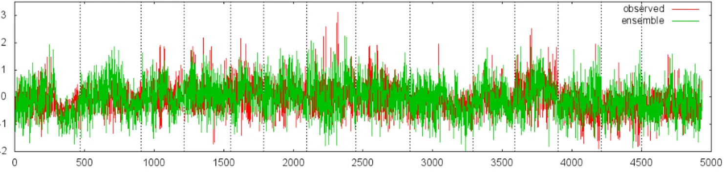
Fig. 3. LM ensemble for MRNBX rolling pullout using biased sampling.
simpler models could be constructed using the MOGA masks without sacrificing performance.
For a thorough comparison, the results from the complemen-tary mask models are also included in Table I. These models were all trained using only the predictor variables that the MOGA discarded. However, the results show that a model for this sensor and flight condition was still feasible, albeit at a much lower level of performance than the full mask. In both training and testing, the ensemble from the complementary mask models yielded a much higher RMSE and lower correla-tion than the best mask models. This difference in performance gives further credence that the variables chosen by the GA had higher predictive power than others.
B. Comparison of Sampling Techniques
The use of the two sampling schemes (k-leaders and biased) to create the training and testing sets led to some interesting differences in the results. The MOGA experiments run in the data exploration stage yielded masks that significantly reduced the number of predictor variables required for the case of k-leaders sampling. This large reduction was observed for both sensors and both flight conditions. Remarkably, some variables appeared consistently between masks, perhaps indicating the possibility of a generalized model. In the case of the biased sampling regime however, there was no evidence of either this reduction in mask size, nor consistency within the predictor variables. Generally, the masks chosen using biased training data had more parameters than their k-leader counterparts: for example, 68 vs. 26 variables in MRNBX rolling pullout, and 84 vs. 26 for MRPR1 rolling pullout.
Despite the increased model complexity from using larger masks, this biased sampling approach still posed as an attrac-tive option for the purposes of helicopter lifetime estimation. As the damage induced by helicopter loads is largely dictated by the peak values in the load signal, training the network to more accurately capture peaks would in theory lead to a better resulting damage prediction. It was thought that this advantage might also lead to overpredicting the less extreme signals present in the testing dataset, so that one would expect a larger testing RMSE. However as mentioned previously, overprediction of the target signal is preferable to
underprediction for the purposes of helicopter load estimation to ensure a conservative estimate.
Surprisingly, the models created using biased training sets did not result in an increased RMSE from overprediction as expected. Quite the opposite, the time series signal as a whole seemed to be better represented using this training set than with the k-leaders training set. Table II shows the results from the deterministic optimization (DO) ensembles for the MRNBX and MRPR1 signals during the rolling pullout ma-noeuvre. In all cases, the ensemble candidates used Levenberg-Marquardt as the learning method. In the instance of the MRNBX signal, the RMSE of the biased set was approxi-mately 30% lower than the k-leader set in training, and about 35% lower in testing. Meanwhile, the correlation was much better in training for the biased set but became comparable in testing. While any difference in correlation would affect the RMSE, the fact that they had similar correlation values but different RMSEs could be loosely interpreted as the k-leaders based prediction was much more ‘squashed’ than the biased prediction. A similar pattern could be seen for the MRPR1 sensor, where the training RMSE was 50% better in training, and 25% better in testing. It is worth noting that although CJ was among the learning methods tested, all of their models paled in comparison to those trained with LM.
TABLE II
LM TRAINEDNNENSEMBLES: BIASEDSETS VSK-LEADERSSETS FOR
MRNBX & MRPR1IN ROLLING PULL-OUT(ROLL-PO) Training Testing MRNBX # param RMSE corr RMSE corr roll-po-k-leaders 26 0.702 0.700 0.938 0.434 roll-po-biased 68 0.479 0.887 0.608 0.461 MRPR1 # param RMSE corr RMSE corr roll-po-k-leaders 26 0.652 0.763 0.822 0.571 roll-po-biased 84 0.323 0.947 0.617 0.566
As seen in Figure 3, the prediction from the biased sampling for MRNBX rolling pullout had significant coverage over the observed target signal. The dashed vertical lines indicate the boundary between different flight recordings, which were taken over several days. As suggested by the variation in the shape of the time signal from one recording to the next, the rolling pullout maneouvre appeared to vary considerably
de-pending on the pilot, aircraft configuration, and environmental conditions. In addition, each individual record did not appear to be homogenous, that is, each record did not solely consist of data from this flight condition. This observation is likely due to the nature of recording such dynamic manoeuvres, as the recording likely would have included the helicopter’s steady state condition just before and after the manoeuvre, the transitions into and out of the manoeuvre, and the manoeuvre itself. Even with this perceived variation though, the LM ensembles proved to be very robust, capturing the phase of the overall time signal quite accurately. Although the biased training appeared to overcome some of the underprediction seen with the k-leaders, there were still some peak signals not captured by the predicted output (affecting the RMSE). C. Behavior of computational intelligence techniques
Several kinds of model building techniques were used in this study, including extreme learning machines, deterministic optimization, evolutionary computation methods, as well as hybrids of these methods. In this section, the performance of these different approaches are compared. The performance results of all the models for all the cases are listed in Table III. Ensembles were created from the top performing models for each method: deterministic optimization (DO) using only LM or CJ neural networks, PSO including the hybrid and memetic versions with LM or CJ, ELMs, and a general ensemble constructed from the top performing DO and PSO models.
While the neural networks using biased training data did not capture the high and low values of the target signal as well as intended, the ELM networks trained with the same data were somewhat more successful in this regard and in fact overpredicted in some instances. Unfortunately, this overprediction by the ELMs only occurred within certain flight recordings and was not consistent. In the regions that were not overpredicted, the prediction was still quite accurate (based on visual comparison of the predicted and target signal). This disparity between the overpredicted and non-overpredicted regions made interpreting the RMSE and correlation difficult. For example, the ELM ensemble in the case of MRPR1 in rolling pullout had both significant coverage, and overpredic-tion, but had a poor RMSE (0.818) and low correlation (0.389) in testing. Although the DO ensemble had better performance results (RMSE = 0.617, corr = 0.566), upon inspection of the predicted signal it had much poorer coverage. This slight overprediction by the ELM networks came at the expense of network complexity: the ELMs each had 1000 neurons in their hidden layers, as opposed to neural networks with just 7 to 12 neurons in their first (and only) hidden layer.
In general, the ensemble candidates from either LM or PSO-LM coarse and refinement were single layer networks ranging from 7-12 hidden layer neurons. There were some two layer networks with 1 to 4 neurons in the second layer that performed well, but most of the top performing models had a single layer. Interestingly, the memetic versions of the PSO algorithm (with either CJ or LM) did not perform as well as the coarse and refined LM-PSO models. Furthermore,
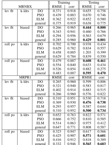
TABLE III
ENSEMBLE RESULTS FORMRNBXANDMRPR1FOR LEVEL FLIGHT AND ROLLING PULL OUT USING K-LEADERS OR BIASED SAMPLING.
Training Testing MRNBX RMSE corr RMSE corr lev flt k-ldrs DO 0.371 0.918 0.655 0.758 PSO 0.439 0.883 0.670 0.746 ELM 0.362 0.922 0.852 0.580 general 0.375 0.919 0.638 0.775 lev flt biased DO 0.266 0.965 0.444 0.800 PSO 0.343 0.941 0.460 0.766 ELM 0.294 0.956 0.563 0.679 general 0.285 0.960 0.429 0.801 roll po k-ldrs DO 0.702 0.700 0.938 0.434 PSO 0.629 0.782 0.834 0.557 ELM 0.458 0.885 1.203 0.399 general 0.629 0.784 0.839 0.550 roll po biased DO 0.479 0.887 0.608 0.461 PSO 0.554 0.840 0.633 0.434 ELM 0.526 0.854 0.882 0.275 general 0.483 0.887 0.595 0.470 MRPR1 RMSE corr RMSE corr lev flt k-ldrs DO 0.265 0.960 0.599 0.806 PSO 0.321 0.940 0.583 0.817 ELM 0.402 0.914 0.883 0.515 general 0.266 0.960 0.576 0.822 lev flt biased DO 0.310 0.951 0.530 0.718 PSO 0.369 0.930 0.476 0.738 ELM 0.293 0.957 0.587 0.644 general 0.310 0.952 0.500 0.734 roll po k-ldrs DO 0.652 0.763 0.822 0.571 PSO 0.666 0.752 0.810 0.585 ELM 0.514 0.863 0.975 0.412 general 0.647 0.771 0.808 0.587 roll po biased DO 0.323 0.947 0.617 0.566 PSO 0.425 0.907 0.571 0.601 ELM 0.416 0.912 0.818 0.389 general 0.332 0.946 0.565 0.603
as was seen with the deterministic optimization models, none of the hybrids with CJ were suitable for the ensemble.
For future studies it may be worth evaluating the damage fraction from the predicted signal generated by each network and comparing it to that of the observed signal, which would give a better indication than RMSE/correlation of which network was better suited for this problem. In addition the introduction of alternative asymmetric error functions in the learning process could be an effective way to encourage overprediction of the signal (and discourage underprediction). D. General Model Ensemble
An ensemble with both PSO and DO models was created for each case, with the hope that combining the two different training methods would overcome any deficiencies seen in the results from each single method alone. The ELM results were purposely omitted, since, as mentioned in Section VI-C, including those results would make any gains or losses in performance difficult to interpret. The results from the general ensemble model for each case are included in Table III.
As expected, some small improvements over the PSO/DO ensembles were seen using the general ensemble model. In spite of this improvement seen by combining methods, the improvement in the k-leader results was still insufficient to outperform the original PSO/DO biased training ensembles,
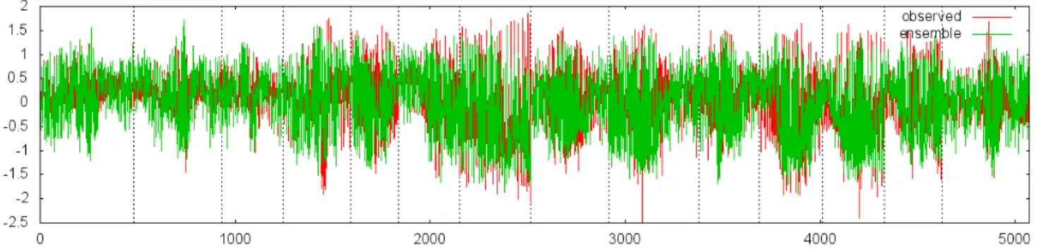
Fig. 4. Generalized model for MRPR1 rolling pullout using biased sampling.
never mind the generalized ensembles using biased sampling. Much like the k-leader results, the performance of most generalized ensembles for the biased set was augmented by combining the PSO and DO models.
Overall, the predictions for level flight were quite good for both main rotor normal bending and the pushrod axial load. As compared to previous results [1] for MRNBX level flight that used an ensemble of M5 model trees and Broydon-Fletcher-Goldfarb-Shanno (BFGS) neural networks (RMSE = 0.593, corr = 0.801), the biased sampling general ensemble model in this work substantially improved the prediction (RMSE = 0.429, corr = 0.801). Prediction of the rolling pullout manoeuvre was a more challenging task and not surprisingly the performance (RMSE/correlation) was not as strong. This manoeuvre was chosen because it is a complex and dynamic flight condition and it is a fatigue damaging manoeuvre for some components. However, as seen in Figure 4 showing the prediction for rolling pullout for MRPR1, the general ensemble model yielded an excellent prediction for the time signal, capturing the peak values quite well in many cases particularly at the extreme values which are the areas most critical for helicopter structural integrity. The fact that reasonable results could be found for this difficult manoeuvre is very encouraging.
VII. CONCLUSIONS
This work expanded the use of computational intelligence techniques and sampling methods to predict several main rotor loads on the Black Hawk helicopter through a broader range of flight conditions. The results found that using a smaller subset of FSCS parameters generated models that performed similar if not better than models that used all the available FSCS parameters. Using a biased sampling scheme to form the training dataset led to larger masks but overall better predictions of the main rotor loads, particularly at the peak values (most critical for helicopter structural integrity). From the wide range of computational intelligence techniques used for building models, the Levenberg-Marquardt neural networks and those paired with particle swarm optimization provided the best performance. The results achieved in this study are quite encouraging as reasonably accurate and correlated models were found for the two flight conditions in spite of
the complexity of the manoeuvres. In addition, the overall quality of the predictions improved through the use of the explored techniques as underprediction of the signal was less frequent. Future work will aim to further improve the predictions by incorporating fatigue damage calculations based on the predicted loads, constructing general models applicable to any flight condition, and using alternative error measures for guiding the learning process.
REFERENCES
[1] J. J. Valdes, C. Cheung, and W. Wang, “Evolutionary computation methods for helicopter loads estimation,” in Proc. IEEE Congr. on Evol. Computation, New Orleans, LA, USA, June 2011.
[2] ——, “Computational intelligence methods for helicopter loads estima-tion,” in Proc. Int. J. Conf. on Neural Networks, San Jose, CA, USA, Aug 2011, pp. 1864–1871.
[3] Georgia Tech Research Institute, “Joint USAF-ADF S-70A-9 flight test program, summary report,” Georgia Tech Research Institute, Tech. Rep. A-6186, 2001.
[4] A. Jones, D. Evans, S. Margetts, and P. Durrant, “The gamma test,” Heuristic and Optimization for Knowledge Discovery, 2002.
[5] A. Stef´ansson, N. Kon˘car, and A. Jones, “A note on the gamma test,” Neural Computing and Applications, vol. 5, pp. 131–133, 1997. [6] D. Evans and A. Jones, “A proof of the gamma test.” Proc. Roy. Soc.
Lond. A, vol. 458, pp. 1–41, 2002.
[7] M. Anderberg, Cluster Analysis for Applications. London UK: John Wiley & Sons, 1973.
[8] W. Pres, B. Flannery, S. Teukolsky, and W. Vetterling, Numeric Recipes in C. Cambridge University Press, 1992.
[9] G. Huang, Q. Zhu, and C. Siew, “Extreme Learning Machine: Theory and Applications,” Neurocomputing, vol. 70, pp. 489–501, 2006. [10] G. Huang, L. Chen, and C. Siew, “Universal approximation using
incremental constructive feedforward networks with random hidden nodes,” IEEE Trans. Neural Netw., vol. 17, pp. 879–892, 2006. [11] L. P. Wang and C. R. Wan, “Comments on ¨the extreme learning
machine¨,” IEEE Trans. Neural Netw., vol. 19, pp. 1494–1495, 2008. [12] Y. H. Pao, Adaptive Pattern Recognition and Neural Networks. Reading,
MA: Addison-Wesley, 1989.
[13] G. Huang, “Reply to Comments on The Extreme Learning Machine,” IEEE Trans. Neural Netw., vol. 19, pp. 1495–1496, 2008.
[14] P. Courrieu, “Fast computation of moore-penrose inverse matrices,” Neural Inform. Process. - Lett. and Reviews, vol. 8, pp. 25–29, 2005. [15] V. Katsikis and D. Pappas, “Fast computing of the moore-penrose inverse
matrix,” Electron. J. Linear Algebra, vol. 17, pp. 637–650, 2008. [16] J. Kennedy and R. C. Eberhart, “Particle swarm optimization,” in Proc.
IEEE Int Joint Conf on Neural Networks, vol. 4, 1995, pp. 1942–1948. [17] J. Kennedy, R. C. Eberhart, and Y. Shi, Swarm Intelligence. Morgan
Kaufmann, 2002.
[18] M. Clerc, Particle Swarm Optimization. ISTE Ltd, 2006.
[19] Y. Zheng, L. Ma, L. Zhang, and J. Qian, “Study of particle swarm optimizer with an increasing inertia weight,” in Proc. World Congr. on Evol. Computation, Canberra, Australia, Dec 2003, pp. 221–226.