Biologically-plausible six-legged running : control and simulation

Biologically-Plausible Six-Legged Running:

Control and Simulation

by

Matthew David Malchano

Submitted to the Department of Electrical Engineering and Computer

Science

in partial fulfillment of the requirements for the degree of

Master of Engineering in Electrical Engineering and Computer Science

at the

MASSACHUSETTS INSTITUTE OF TECHNOLOGY

February 2003

@

Matthew David Malchano, MMIII. All rights reserved.

The author hereby grants to MIT permission to reproduce and

distribute publicly paper and electronic copies of this thesis document

in whole or in part.

A uthor ...

Department of Electrical Engineering and Computer Science

February 4, 2003

Hugh M. Herr

Instructor, MIT/Harvard Division of Health, Science, and Technology

Thesis Supervisor

Accepted by...

Arthur C. Smith

Chairman, Department Committee on Graduate Students

MASSACHUSETTS INSTITUTE OF TECHNOLOGY

Biologically-Plausible Six-Legged Running: Control and

Simulation

by

Matthew David Malchano

Submitted to the Department of Electrical Engineering and Computer Science on February 4, 2003, in partial fulfillment of the

requirements for the degree of

Master of Engineering in Electrical Engineering and Computer Science

Abstract

This thesis presents a controller which produces a stable, dynamic 1.4 meter per sec-ond run in a simulated twelve degree of freedom six-legged robot. The algorithm is relatively simple; it consists of only a few hand-tuned feedback loops and is defined by a total of 13 parameters. The control utilizes no vestibular-type inputs to actively control orientation. Evidence from perturbation, robustness, motion analysis, and parameter sensitivity tests indicate a high degree of stability in the simulated gait. The control approach generates a run with an aerial phase, utilizes force information to signal aerial phase leg retraction, has a forward running velocity determined by a single parameter, and couples stance and swing legs using angular momentum infor-mation. Both the hypotheses behind the control and the resulting gait are argued to be plausible models of biological locomotion.

Thesis Supervisor: Hugh M. Herr

Acknowledgments

Hugh Herr, Gill Pratt, and Max Berniker, Joaquin Blaya, Bruce Deffenbaugh, Pete Dilworth, Jon Gonda, Andreas Hofmann, Frank Kirchner, Marko Popovic, and Rebecca Schulman:

Thanks much, y'all.

Mom, Dad, and Zach Malchano: My love.

Contents

1 Introduction 13

2 Background Material 15

2.1 A Short Introduction to Running . . . . 15

2.2 Biological Inspiration . . . . 15

2.3 Hexapedal Robots . . . . 16

3 Hexapedal Running Control Algorithm 19 3.1 Introduction . . . . 19

3.2 Morphology . . . . 20

3.3 Running Control Algorithm . . . . 22

3.3.1 Aerial Phase Control . . . . 22

3.3.2 Stance Phase Control. . . . . 25

3.4 Details of Methodology . . . . 28 4 Results 29 4.1 Motion Analysis . . . . 30 4.2 Perturbation Testing . . . . 34 4.3 Robustness . . . . 38 4.4 Parameter Sensitivity . . . . 40 4.5 Biological Plausibility. . . . . 42

5 Conclusions and Future Work 45 A Mechanical Designs 47 B Control Source Code 51 B .1 6legs.h . . . . 54

B.2 create-hexahop.c . . . . 55

B .3 bug lhop.h . . . . 58

B .4 bug lhop.c . . . . 58

List of Figures

3-1 The hexapod model. . . . . 19 3-2 Diagram of hexapod model joint configuration, view from sagittal plane 21

3-3 Block diagram of aerial phase control . . . . 24

3-4 Block diagram of stance control . . . . 27

4-1 Mean kinematic motions of the center of mass, system potential and kinetic energies, and pitch-axis angular momentum. . . . . 31 4-2 Mean ground reaction forces: horizontal and vertical components for

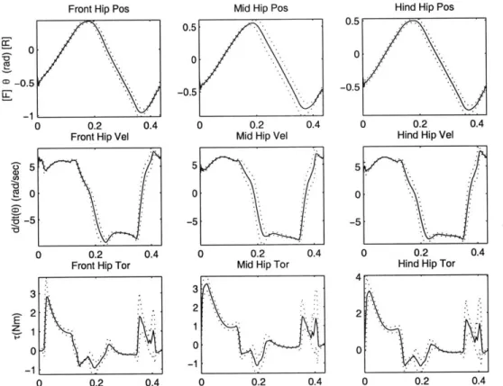
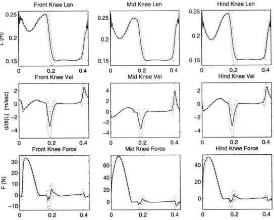
front, middle, and rear legs of a tripod. . . . . 31 4-3 Mean hip joint kinematics: angle, angular rate, and torque. . . . . . 32 4-4 Mean knee joint kinematics: leg length, velocity, and applied force. 33

4-5 Mean mechanical joint power output. . . . . 33

4-6 Impulse torque perturbations: resulting momenta vs. time . . . . 35 4-7 Horizontal impulse force perturbation: resulting linear and angular

m om enta. . . . . 36 4-8 Vertical impulse force perturbation: resulting horizontal and vertical

linear m om enta. . . . . 37 4-9 Robustness to initial height and forward velocity . . . . 38 4-10 Robustness to initial pitch and pitch rate of change . . . . 39

A-1 Assembly drawings and section view of first distal segment design. . . 47

A-2 Assembly drawing and section view of revised distal segment . . . . . 49

List of Tables

3.1 Morphological parameters defining the simulated model. . . . . 21

3.2 Aerial phase control parameters . . . . 22

3.3 Stance controller parameters . . . . 25

4.1 Summary of gait measurements. . . . . 30

4.2 Maximum magnitude of step perturbations resulting in stable gait. . 35 4.3 Independent sensitivity of parameter values: minimum, nominal, and maximum values for which a stable gait of more than 10.0 sec results. 40 4.4 Comparison of simulation measurements with biological model predic-tion s. . . . . 42

B.1 Variable names used in simulation source code and coresponding sym-bols from text. . . . . 52

Chapter 1

Introduction

The difficulties of control in legged locomotion are well documented [28]: (1) the high dimensionality and nonlinearity of the dynamics; (2) the relatively short duration of and limited control provided by the ground reaction forces; (3) the complexity of environmental conditions; (4) mechanical limitations in power, bandwidth, and energy efficiency; and (5) operation in a gravitational field. Yet the promise of legged locomotion is obvious in nature's ability to efficiently walk, run, trot, gallop, leap, and bound over most of the Earth's terrain. The lack of machines capable of reproducing this range of biological behaviors is evidence of the numerous challenges still faced by researchers.

Many of the controllers for six-legged (or hexapod) robots exhibit a high level of computational and conceptual complexity. Inverse kinematics, inverse dynamics, and complex models are common features. The systems are defined by large sets of high-precision parameters. The use of computational search methods, nonlinear optimizations, and machine learning techniques is often necessary. The usual focus is the production of a robust walking gait. Almost all of the resulting "hexapod literature has [up until 2001] concerned static or quasi-static walking machines." [2]

Recent successes in legged locomotion have been reported using control techniques labeled "feedforward", "open-loop", or "preflex" [34, 8, 33]. In these techniques, mo-tions are coordinated by a central oscillator or clock. The oscillator triggers the play-back of trajectories at each joint. Often the control targets a highly simplified morphology with only one actuated degree of freedom (dof) per leg. The oscilla-tor frequency, trajecoscilla-tory, and physical parameters are searched computationally or empirically until a satisfactory form of locomotion emerges.

The algorithm presented in this thesis diverges from both the static walkers and the "feedforward" approaches. In contrast to complicated control techniques used in the walkers, the controller studied consists of only a few hand-tuned position and velocity control loops and a two-state finite state machine. These loops servo joints to simple positions or velocities. The hexapod model runs dynamically.

The controller resembles the "feedforward" methodology in its relative simplic-ity and its stabilization without the use of vestibular-type information, such as a gyroscope signal. A number of important distinctions separate this work from the "feedforward" class. The morphology, with two actuated degrees of freedom per leg,

lies between both the 3-dof insect leg design common in statically-stable walkers and the 1-dof legs found in the "feedfoward" morphologies. The control is not a purely clock-driven system, but rather it predicts approximate ground contact time using force information in order to signal leg retraction. A single parameter value selects from a range of forward velocities. Angular momentum information is used to couple stance and swing legs motions. The controller uses the feedback of a few high-level state variables and on-line calculation of dynamic quantities in generating leg trajec-tories. Finally, where "functional biomimesis" of cockroach locomotion inspires many "feedforward" algorithms, the basis for this controller is instead a model of horse trotting [15].

The organization of presentation here is as follows:

1. A short introduction of running locomotion, description of the horse trotting model, and survey of hexapedal control is made in Chapter 2.

2. The main goal of this work is the design of a novel hexapedal running control algorithm. It is described in depth in Chapter 3

3. The resulting motions of the gait produced in simulation, the evaluation of stability through perturbation, sensitivity, and robustness testing, and an argu-ment for biological plausibility may be found in Chapter 4

4. Finally, a summary of the main conclusions and future directions of this thesis occurs in Chapter 5

5. I designed three mechanical leg segments to further physical testing, and they are documented in Appendix A. The controller source code is listed in Ap-pendix B.

Chapter 2

Background Material

2.1

A Short Introduction to Running

A run is a fast locomotory mode characterized by specific motions of the center of mass. In particular, these motions feature significantly in-phase sinusoidal kinetic and potential energies. The simplest model of running which exhibits these energy profiles is the monopod. It consists of a single massless linear stiffness leg and a point-mass body. It has been shown that many animals' legs approximate such linear stiffnesses during running gaits [5]. Additionally, many runs feature an aerial phase: a period during which no feet contact the ground [24]. These characteristics hold true for morphologies running with any number of legs [4, 10].

A common gait used by hexapods, both natural and artificial, is the alternating tripod gait [17]. This symmetric and alternating gait moves legs together in groups of three. The front and hind ipsilateral and middle contralateral legs combine to form a tripod. The legs of a given tripod alternate between stance phase (during which they contact the ground) and swing phase (during which they move forward through the air).

Gaits, including running gaits, may be divided into those that are statically stable and those that are dynamically stable. This terminology was introduced by [23]. The points of ground contact of the stance legs define a support polygon. In a statically stable gait, the center of mass always lies directly above this polygon. In a dynamically stable gait, on the other hand, center of mass projects outside of this polygon for some significant portion of the gait cycle. The gait then relies on its momentum to carry it through these periods of instability. Cockroaches, even though six-legged, move dynamically [12].

Given these above definitions, the hexapod presented in this thesis may be said to move in a dynamically-stable, alternating-tripod running gait.

2.2

Biological Inspiration

A biological model of horse trotting [15] provides the initial basis for the running controller presented in this work. This quadrupedal model has been shown to

suc-cessfully predict biologically observed metrics across a range of masses [14], and has been further adapted to model horse galloping gaits [16].

Trotting is a gait where diagonal limb pairs alternately strike the ground. This pairing resembles the motions of a hexapedal alternating tripod gait, where limbs are also grouped diagonally. Trotting occurs as a middle speed gait between walking and galloping in a variety of quadrupedal animals. The central ideas posed in the trotting model are:

1. Both diagonal limbs in a pair begin retraction simultaneously.

2. A trotting animal estimates when its feet will first strike the ground and begins limb retraction at this time. Hence, retraction may occur before foot contact. This estimation is performed on-line using the previous stance phase pitch and force information. It is believed that beginning retraction before ground contact may help stabilize those gaits which may be modeled as monopods [35], such as trotting and hexapedal running.

3. Stance leg retraction attempts to match a tangential target speed.

4. Vertebrate limbs behave like linear stiffness springs during ground contact.

5. Hind hip joints provide motive force. Forward hip joints provide braking force. 6. No active control of body orientation is used.

The trotting study was conducted using sagittal planar models. These models possessed 4 radially compliant legs with rotary hip joints; back and neck joints with passive stiffnesses were included to replicate the horse morphology accurately. Sta-bility was evaluated based on the number of gait cycles the simulation locomoted without significant change to pitch, aerial apex height, or forward velocity. Addition-ally, simulations were subjected to a ground impedance change while trotting to test disturbance rejection.

The above ideas provide both the inspiration and starting framework for this work. Specific documentation of divergences and modifications may be found in Chapter 3.

2.3

Hexapedal Robots

This section seeks to place this thesis' contribution in the context of other work in hexapedal control. The histories of the study of legged locomotion are long and broad, and more detailed accounts of the robotics [31], biomechanics [24], and recent

advances [32] may be found elsewhere.

The literature documents numerous approaches specific to hexapedal control. These approaches have focused mainly on producing robust walking gaits in 3-dof per leg morphologies. The advanced concepts and computational methods are ap-plied. Parameter search techniques have been used to reduce the complexity of the resulting controllers. For example, neural nets [3], genetic algorithms [22], and vari-eties of reinforcement learning [18] have been used to define parameters. The problem

has been decomposed into a variety of subproblems, with restricted goals such as gait generation [39], fault tolerance [41], rough terrain navigation [40], and leg coordina-tion [1]. Biological organisms have served as physical [38, 26] as well as behavioral models [11]. Many of these controllers are successful in their chosen objectives or introduce innovative approaches. Yet all of these hexapods, along with many oth-ers, locomote in only static or quasi-static regimes. Their focus includes neither fast

running gaits nor simplicity.

The MIT Leg Lab has previously developed two six-legged walking simulations similar to the aforementioned systems. The first controller targets a cockroach-sized morphology and uses a technique called "virtual model control" [37]. In virtual model control, desired forces are prescribed to the body link. For example, a "virtual" linear spring, attached between the center of mass and a "virtual" fixed frame, might counteract gravity's force on the body. The leg inverse kinematics and the Jacobian are used to map these "virtual" forces to leg joint torques, which exert real forces against the ground to produce the desired motion. The second hexapod, a simulated automobile-sized walking vehicle, also relies on this technique [27]. Neither controller claims biological plausibility.

More recently, impressive successes have been had in a series of highly simplified approaches. These approaches are unified in their use of a clock to coordinate the playback trajectories on 1-dof actuated legs and their emergent passive stability. They are also unified by their "functional biomimesis" of cockroach locomotion. Below I discuss RHex [2, 34], Sprawlita [8, 6], and Wheg [30], three examples of this approach to control.

The autonomous robot RHex possesses six actively controlled degrees of freedom, one per leg. The actuation is provided by rotary hip joints whose axes lie perpen-dicular to the sagittal plane. Legs move in complete rotations and group together in alternating tripods. A central oscillator coordinates the hips, which use local feed-back loops to follow one of two velocities: a "retraction" velocity for stance phase and a faster "protraction" velocity for swing phase. Buhler et al. report a forward gait, with a speed of one body length per second, emerges after physical tuning of the system mass, leg spring stiffness, target velocities, and loop gains.

Sprawlita is a pneumatically actuated, tethered robot. It's 1-dof legs are pneu-matic cylinders attached to the body with passive stiffnesses. In Sprawlita, a central pattern generator again sends a periodic feedforward trajectory to the mechanical system. Cham et al. argue passive stiffnesses and pneumatic cylinders act as purely mechanical feedback (termed "preflexes") which stabilize the gait. Otherwise, no feedback occurs. The controller may also servo the angle of all hips, but does not do so during intra-stride operation. The feedforward trajectory is a simple "bang-bang", extend-or-retract command sent to all legs in a tripod. The frequency and duty cycle of this trajectory were determined empirically. Sprawlita has been shown to move at speeds of 2.5 body lengths per second.

Wheg uses a morphology similar to RHex but with three radial-stiffness spokes per leg instead of one. Additionally, it reduces leg drive to a single motor. Its controller appears similar to RHex, but targets only a single angular rate per leg and switches its legs to an in-phase gait when climbing obstacles. It's forward velocity is

undocumented.

Since the initial work on both Sprawlita and RHex, additional research has begun adding high-level adaptive feedback to these systems. In RHex, body orientation and foot contact information has been used to adjust for ground slope conditions [20]. This information is also being used to research adding an aerial phase to RHex's gait. In the above, Komsuoglu et al. state that, "experimental observations suggest higher forward speeds can be achieved provided an aerial phase is introduced....". In Sprawlita, a foot contact signal was used to modify the frequency and duty cycle of the feedforward trajectory to aid slop ascent

[7].

Both of these recent incremental successes, I believe, validate the direction of the work pursued in this thesis, which utilizes a different set of high-level feedback terms in a simple control system.

Chapter 3

Hexapedal Running Control

Algorithm

3.1

Introduction

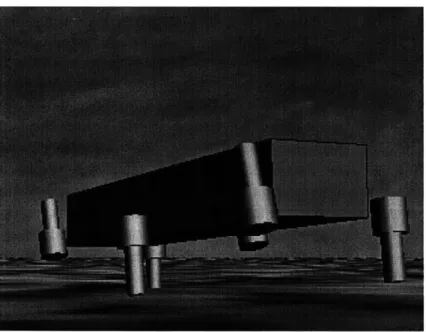
Figure 3-1: The hexapod model.

The control algorithm presented in this chapter generates leg motions in the above 12-dof model (Figure 3-1). These leg motions in turn produce a fast tripod running gait in simulation.

What are the salient features of this control? It is coordinated by a finite state machine. Foot contact switches signal FSM state changes. Proportional gain or proportional-derivative feedback loops mostly servo joints to constant positions or velocities. No active mechanism maintains body orientation; instead, level posture

emerges passively. Leg retraction matches the distal leg end velocity to the target forward velocity. Angular momentum information about the stance leg is used to coordinate opposing swing leg motion. Leg retraction occurs based on an on-line prediction of ground contact time. The resulting gait possesses an aerial phase. The rest of this chapter gives precise description of these features.

Simulations of sagittal-planar and fully three-dimensional models were developed for a variety of masses. The results contained in this thesis focus only on the sagittal-planar model. The hexapedal sprawled posture causes most of the interesting dy-namics to occur in the sagittal-plane. Reduction of orientation state to only pitch angle and derivatives allows a clear examination of the degree of passive orientation stability. For the three-dimensional simulations, only small changes to leg sprawl and increases in hip gains were necessary to achieve stable locomotion.

Section 3.2 describes the model used in simulation. The control algorithm is dis-cussed in detail in Section 3.3. As previously mentioned, this work draws inspiration from a model of quadrupedal trotting. Documentation of the specific differences be-tween these systems, along with various notes on simulation development, may be found in Section 3.4.

Results analyzing the gait produced by this control follow in Chapter 4. The complete source code for the controller, along with some supporting simulation code, may be found in Appendix B.

3.2

Morphology

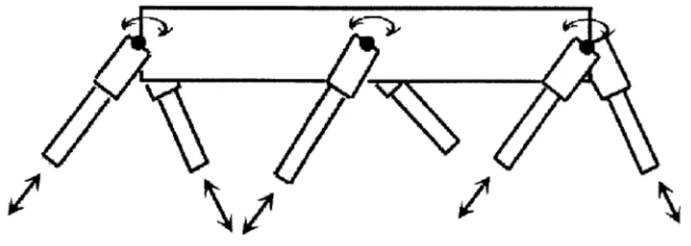
The hexapod model possesses 12 actuated degrees of freedom. Each leg has a rotary hip whose axis lies perpendicular to the sagittal plane and a prismatic knee oriented radially from that hip. The hip joints attach the thigh link to the body, with fore and hind hips located at the body's corners and at the vertical level of the body center of mass. Each hip joint acts to protract (swing forward) and retract (swing hindward) a given leg in the sagittal plane. The knee joints attach the thigh to the shin and act to lengthen or shorten the leg. Additionally, during stance phase, these knee joints behave as linear, high stiffness leg springs. Figure 3-2 diagrams these actuated joint motions in the sagittal plane.

An un-actuated joint, co-located with the hip, splays the thighs outward within the frontal plane. A passive 40 N/in stiffness and 20 N-s/in viscosity hold these legs at an angle of 0.1 radians from vertical. The splay and stiffness maintain the necessarily sprawled posture in the 3D simulations.

The hexapod inherits this general form from the quadrupedal trotting model. Similar morphologies also appear in other robots and biomechanical models, such as [31, 25, 36], in part due to common recognition of a tested hypothesis suggesting that the legs of many animals behave like linear-stiffness springs [5].

The physical parameters defining the hexapod are summarized in Table 3.1. The total mass, its distribution, body dimensions, and leg lengths roughly approximate the latest iteration of the Scorpion robot [19]. I chose to model these values on the Scorpion because of prospective plans to conduct physical tests using some of its

6A

Figure 3-2: Diagram of hexapod model joint configuration, view from sagittal plane

hardware. mass and

One consequence of this choice, the legs total nearly hence contribute significantly to the system dynamics.

Parameter Symbol Value Unit

Body mass - 3.104 kg

Thigh mass Mthigh 0.464 kg

Shin mass Mshin 0.029 kg

Total mass 6.062 kg Body length - 0.64 m Body height - 0.10 m Body width - 0.145 m Thigh length Lthg9h 0.076 m Thigh radius - 0.15 m Shin length Lshin 0.176 m

Shin radius - 0.024 m

Max Leg Length - 0.252 m

Min Leg Length - 0.052 m Max Hip Angle - 7r/2 rad

Min Hip Angle - -7r/2 rad

50% of the system

3.3

Running Control Algorithm

This section discusses the control algorithm which generates the hexapod's running gait. A centralized controller coordinates the motions of the legs. This controller is in one of two states during steady state locomotion: aerial phase (Section 3.3.1) or

stance phase (Section 3.3.2). Each state performs a separate function. In the aerial

phase, the hexapod moves in a ballistic trajectory through the air. The controller positions the legs to prepare for ground contact. During the stance state, the hexapod contacts the ground, and the controller moves the legs in order to propel the body forward and upward into the air.

In both states, the legs are grouped into two tripods of three legs each. Each leg in a tripod is commanded similarly. At any time, one of the tripods is designated the stance tripod and the other the swing tripod. During stance phase, the legs of the stance tripod are in contact with the ground, while the legs of the swing tripod do not touch the ground. When control switches from the stance phase to the aerial phase, the designations for the tripods are swapped. The swing tripod becomes the stance tripod and vice versa. Hence, in aerial phase, the tripod designated as the stance tripod will contact the ground in the subsequent stance phase.

3.3.1

Aerial Phase Control

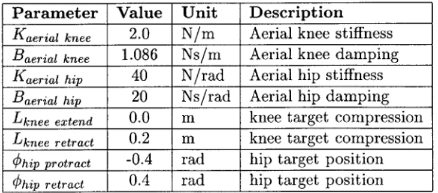
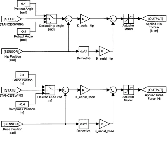
Aerial phase control positions the legs to prepare the hexapod to enter into stance phase control. Aerial phase control begins when the hexapod's leg leave the ground and ends when ground contact is predicted to occur again. During aerial phase con-trol, the legs are positioned to a ready position for the next stance phase's initiation. Figure 3-3 shows the aerial phase controller for both knee and hip joints in block diagram notation. Table 3.2 lists the numerical values of the controller gains and target positions.

Parameter Value Unit Description

Kaerial knee 2.0 N/m Aerial knee stiffness

Baerial knee 1.086 Ns/m Aerial knee damping

Kaerial hip 40 N/rad Aerial hip stiffness

Baerial hip 20 Ns/rad Aerial hip damping

Lknee extend 0.0 m knee target compression

Lknee retract 0.2 m knee target compression

Ohip protract -0.4 rad hip target position

khip retract 0.4 rad hip target position

Table 3.2: Aerial phase control parameters

At the beginning of the aerial phase, the swing tripod starts in a retracted position and with its knees fully extended. The stance tripod starts protracted and with its knees fully compressed. Proportional-derivative position control loops at the hips

apply torques to both tripods to brake the inertia from the previous stance phase's motions and to roughly position the tripods for entry into the next stance phase. The target angle for the stance tripod protraction was estimated by considering the return path of a spring-mass monopod dropped from the predicted average height of the hexapod center of mass apex and with the predicted velocity of the hexapod robot. The angle of attack of this monopod was used as the target protraction angle. This value was then hand-tuned until a steady state run in the hexapod model was achieved. The same angle from vertical is used for the swing tripod target retracted position.

Hip loop gains were chosen to assure that legs were brought to a halt before they contacted the hip joint stops. Although it was intended that loop gains would be high enough to assure precise positioning to the desired target positions before the end of aerial phase, this behavior was not observed in the final simulation. Instead, some variation in protracted leg position was observed. Hip damping coefficients were chosen to critically damp the motion of the hips, assuring that no oscillation or overshoot occurs during leg motion.

When aerial phase is entered, the controller estimates the time of the next ground contact, which is when stance phase should start. This estimation is accomplished using the vertical velocity of the center of mass of the hexapod at the moment aerial phase begins. From this, the duration of a parabolic flight path during aerial phase is predicted. A timer maintains the elapsed time from the onset of aerial phase control; when the timer exceeds the predicted duration, aerial phase ends and stance phase begins. The controller also switches into stance phase if a leg contacts the ground at any time during aerial phase motion.

Just before aerial phase control ends, P-D controllers apply forces to the knees to extend the stance tripod to its maximal length and compress the swing tripod by 0.15 meters. Knee gains and damping coefficients were chosen to assure this motion completes before ground contact.

S 0.4

Protract Angle [rad]

[STATE] +_K +_a[OUTPUT]

STANCE/SWING Desired Hip Angle K aerial hip Actuator Applied Hip

-m 4 [rad] Model Torque [m4lrd [Nm Retract Angle [rad] [SENSOR]

Hip Position _{Derivative Baerialhip}

[rad]

F

0.4

Extend Positon

[m]

STAE]N +_pie KK+n[UTUT

STNC/WIG Desire Ke Plos K aerial knee Actuator Applie KNe

[m] Mde Force [N]

-0.4 Compress Position

[m]

|[SENSORI ud

Knee rPosition Derivative B aerial knee

3.3.2

Stance Phase Control

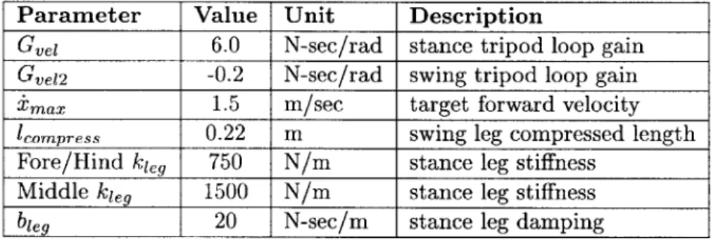
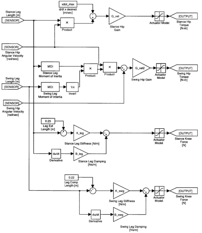
Stance phase control determines the motions of the tripods during ground contact. The stance tripod usually contacts the ground shortly after the onset of stance phase control, and the control ends when that tripod again leaves the ground. During this control, the stance tripod moves from a protracted position to a retracted position and acts against the ground. Simultaneously, the swing tripod moves from a retracted position to a protracted position without contacting the ground. Figure 3-4 shows a control block diagram depiction of the control used during stance phase. Table 3.3 lists the gains and desired velocities used in the controller.

Parameter Value Unit Description

Gvel 6.0 N-sec/rad stance tripod loop gain

Gve12 -0.2 N-sec/rad swing tripod loop gain

Xmax 1.5 m/sec target forward velocity

1

compress 0.22 m swing leg compressed length

Fore/Hind kleg 750 N/m stance leg stiffness Middle kie, 1500 N/m stance leg stiffness

bleg 20 N-sec/m stance leg damping

Table 3.3: Stance controller parameters

Stance phase control begins when either the predicted duration of the aerial phase expires or when one or more legs contact the ground. In normal steady-state behavior, stance phase initiates slightly before ground contact. This preliminary acceleration results in "leg retraction", which was one of the hypotheses posed in the quadruped model.

At the initiation of stance phase control, knees begin to act as high linear stiff-nesses. The front and hind stance legs are set to a 750 N/m stiffness with 20 N-sec/m damping coefficient. The middle leg switches to a 1500 N/m stiffness; this stiffness is doubled to compensate for the asymmetry of the tripod. Without this adjustment, asymmetrical ground reaction forces, a body-roll moment, and insufficient rear leg ground clearance occur during stance. Swing tripod knee stiffness also increase.

The hips of the stance tripod are controlled with proportional velocity loops. These loops attempt to match the distal end of a stance leg's tangential speed to the ground speed for speeds less than the desired forward velocity imax. The distal end

of the leg has a velocity of v = Ileg *

#hip

#hip(t)

Thip(t) = Gvei * ((lieg(t) - hip(t)) - Ximax) (3.1)

The swing leg control operates as follows. Proprioception information provides the compression of the stance leg Alstance(t), along with the velocity of the stance leg

for the stance leg about the hip joint is calculated:

Istance I Mthigh - (0.5 -Lthigh )2 + Mshin - (0.5Lihin - Lthigh - Alstance(t)) 2 (3.2)

Hence, the angular momentum of the leg about the hip axis is

Lh p(t) = 'eg(lieg(t)) -Oip. (3.3)

The target velocity bswing(t) of the stance leg is set to cancel this angular momentum.

Istance (t)

-= Iswing(t) -/Ostance(t) (3.4)

A proportional velocity control loop with negative gain Gel2 servos the swing leg

speed to follow bswing(t). The applied hip torque is

Thip(t) = Gvei2 -(bswing(t) + swing (t)). (3.5)

Since the swing leg length is always shorter than the stance leg length, Ising(t) <

Istance(t) and therefore iswing(t) > &ance(t). The swing leg will hence be in position

to enter aerial phase. We suspect that angular momentum about the center of mass plays an important role in dynamically stable locomotion. Swing leg control annuls the pitch-axis angular momentum about the hip, but this is only the smaller of the two terms expressing the effects of a leg's contribution to the angular momentum in the body frame. Further research is necessary before these speculations can be confirmed.

The control outlined above for the hip and knee joints is maintained throughout stance phase. Stance phase ends when all feet leave the ground. At the transition, the controller starts the aerial phase timer, records the vertical velocity, and switches stance and swing tripod designations. It then enters aerial phase.

ty

Mx _x

G_ve12 _[PTPT

Stance Leg Product Actuator Swing Hip

Moment of Inertia Product. Torque

Swing Hip Gain Mdl [N-m]

Swing Leg Invert Moment of Intertia

ty

[OUTPUT]

Actuator Stance Knee

Model Force [N] 0.25 Leg Ext Length [m] K-leg-,

Stance Leg Stiffness J[N/m]

Derivative _{Stance Leg Damping} [Ns/m]

[0.22

Leg Comp

Length [m]

+ ~ Kswg -, [OUPUT]

Actuator Swing Knee Swing Leg Stiffness Model. Force

[N/m] [N]

d/t B-swg

Derivative

Swing Leg Damping [Ns/m]

Figure 3-4: Block diagram of stance control Stance Leg Length [m] [SENSOR]

ESENSOR]

-x Actuator Model Stance Hip

Stance Hip Torque

3.4

Details of Methodology

The control presented here uses the quadrupedal model as inspiration, but both morphology and control differ in a number of very significant ways. The hexapod morphology adds two legs, makes the body link rigid, and removes the head link. The mass, mass distribution, and dimensions have all been changed. Viscous damping has been added to the hexapod's stance leg springs to model mechanical losses.

Control differs from the quadruped as follows. Symmetric target velocities and stiffnesses are used for fore- and hindlimbs; in the quadruped these targets are sig-nificantly different. The aerial state occurs when all feet leave the ground; in the quadruped it occurs when any single foot loses contact. Only vertical take-off speed is measured to predict ground contact; the quadruped also uses pitch sensor infor-mation. The swing leg follows the opposing stance leg's angular momentum; the quadruped's swing leg "mirrors" the position of the stance leg instead. Parameter values differ widely. The quadrupedal model documents that twenty-eight unique velocities, stiffnesses, gains, and feedback targets define its control. The hexapod control is defined by thirteen such quantities.

Simulations were developed in Creature Library [21], an MIT Leg Lab extension to the commercial dynamics simulator SD-Fast [9]. A 4th-order Runge-Kutta integrator integrated the equations of motion generated by SD-Fast with a 200 nsec step size. The ground model was a linear spring and damper system with a stiffness of 400 N/in and a viscosity of 100 N-sec/m.

All simulation results reported relied on hand-tuned control parameters. At one point, I attempted to computationally generate parameters using naive nonlinear optimization. The optimization attempted to minimize the basic cost function

V = 1 (-i(t) - Xd)2 + (z(t) - Zd)2 + (t)2 _(3.6)

to<t<tf

with V evaluated using the simulation. In the case of instability, out of range param-eters, or other failure cases, V defaulted to its maximal value. The search space was over only five controller parameters. Computing an analytical gradient for the system appeared too difficult an undertaking, and hence Powell's method [29] was chosen as the nonlinear optimizer. It generates gradient information by sampling cost function values for changes in each parameter. It then line-minimizes along the direction which appears most promising. Initial parameter values were selected from a known-good starting point.

This approach was proved infeasible due to a number of stumbling blocks. The cost function failed to capture the desired behavior. The optimization seemed to become trapped in local minima. Large portions of the parameter space produce no useful optimization information due to the "brick wall" nonlinearities in the cost function for gait failures. The simulation runs far slower than realtime and an eval-uation of a parameter set requires on the order of tens of seconds of simulated time. Hence optimization trials took a long time. Numerical optimization was eventually abandoned in favor of hand-tuning.

Chapter 4

Results

A mathematically rigorous, analytical evaluation of system stability is not tractable: the high dimensionality, nonlinearity, and dynamic complexity alone limit the ability to present such a treatment. Even if it were possible, the the value of the analyses obtained would be questionable. Yet, the existence of a stable gait in simulation pro-vides thin proof unless its ability to handle the wide range of environmental conditions found in the real-world is demonstrated.

This chapter presents evidence that argues for the system's convergence to a steady-state periodic gait over a range of initial conditions, in the presence of distur-bances, and with an insensitivity to changes in parameter values. These tests offer a compelling argument that the algorithm exhibits long-term stability and is physically realizable.

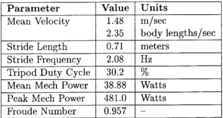
Simple metrics of the resulting gait (Table 4.1) allow performance comparison to other legged locomotion algorithms. Mean kinematic traces for joints and the center of mass motions describe periodic steady-state behavior (Section 4.1) . Error bars on these kinematic traces provide information as to the typical divergence seen from this mean motion. Torque and force perturbations quantify disturbance rejection (Section 4.2). Robustness testing samples the space of initial conditions to deter-mine those which result in steady-state motion (Section 4.3). Parameter sensitivities measure the necessary precision of the values defining the controller (Section 4.4). Finally, the biological plausibility of the algorithm is discussed (Section 4.5).

Throughout this chapter, a gait is termed stable or in a periodic steady state if, over some stated period of time, the gait occurs without a gait failure. A gait failure is defined as body ground contact or joint torques exceeding simulation integration limits. The system is considered stable if it exhibits a stable gait. Additionally, when initial conditions of a simulation are not given, it may be safely assumed they are standard initial conditions: J = 0.7 m/s; z = 0.3 m; 0 = 0.0 rad; 0 = 0.0 rad/sec;

Parameter Value Units

Mean Velocity 1.48 m/sec

2.35 body lengths/sec

Stride Length 0.71 meters Stride Frequency 2.08 Hz

Tripod Duty Cycle 30.2 %

Mean Mech Power 38.88 Watts Peak Mech Power 481.0 Watts

Froude Number 0.957

-Table 4.1: Summary of gait measurements.

4.1

Motion Analysis

The gait analysis plots below display the mean motions of the hexapod during steady-state locomotion over a single gait cycle. This gait cycle includes the stance phases of both tripods along with two aerial phases and lasts an average duration of 0.435 sec. The stance phase for one tripod begins at t = 0.00 sec and ends at t = 0.13 sec;

the opposing tripod's stance phase begins at t = 0.21 sec and ends at t = 0.34 sec.

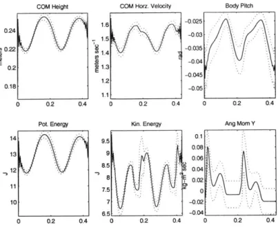
Figure 4-1 shows the motions of the center of mass along with the system's kinetic and potential energy and angular momentum in the center of mass frame.

The remaining plots give leg specific information for the tripod initially entering stance. Since the gait is nearly symmetric, only a single tripod's motions needs be displayed. Figure 4-2 shows the ground reaction forces for the front, middle, and rear legs of this tripod. These forces are split into vertical (z-direction) and horizontal (x-direction) components. Positive horizontal forces point in the direction of robot motion. Figure 4-3 shows the hip joint position, velocity, and force for the same legs. Positive values correspond to retraction. Figure 4-4 shows the knee joint position, velocity, and force. Figure 4-5 shows absolute mechanical power output for the individual joints. These power graphs do not account for regeneration through negative work. They also neglect possible passive mechanical implementations. For example, if the knee joint stiffness in stance phase were implemented with a passive compression spring, no net power output would occur. Previous power numbers do take passive knee implementation into account.

These plots were produced in a standard gait plot format. The data were collected over a 10 second simulation. They were then split into samples beginning at the instant of a specific tripod's first ground contact. These samples were resampled to a uniform length and filtered with a 10-point window, low-pass FIR filter. The mean across these samples was then taken and is plotted as the solid line. The two dashed lines delimit plus and minus one standard deviation from this mean. Some minor high-frequency noise is visible at the edges of a few of the plots. This noise is believed to be an artifact of the FIR filter; it should be stressed that it does not result from any system motion or dynamics.

COM Height 0.24 E 0.22 0.2 0.18 0 0.2 0.4 Pot. Energy 14 13 12.. 11 10 0 0.2 0.4 1.6 -1.5 '0 1.4 E 4)1.3 1.2 1.1

COM Horz. Velocity

0 0.2 0.4 Kin. Energy 9.5 9. 8.5 8 7.5 71 6.5 0 0.2 0.4 -0.025 -0.03 0.04 -0.0 Body Pitch 5 0 0.2 0.4 Ang Mom Y 0.1 0.08 0.06 0.04 0.02 0 -0.02 -0.04 -... 0 0.2 0.4

Figure 4-1: Mean kinematic motions of the center of mass, system potential and kinetic energies, and pitch-axis angular momentum.

Z 40 30 20 z 10 0 GRF Front Leg (x) 2. 0 0. 0 0.2 0.4 GRF Front Leg (z) 0 0.2 0.4 z GRF Middle Leg (x) 5 0 -5 -10 0 0.2 0.4 70-60 50 40 z3 20 10 0 0 GRF Middle Leg (z) 0.2 0.4 GRF Hind Leg (x) 5 z 0 -5 0 0.2 0.4 GRF Hind Leg (z) 50 40 30 z 20 10 0 0 0.2 0.4

Figure 4-2: Mean ground reaction forces: horizontal and vertical components for front, middle, and rear legs of a tripod.

-Front Hip Pos

0'

--0.5

0 0.2 0.4

Front Hip Vel S5

0.

-5

-5

0 0.2 0.4 Front Hip Tor

3

2

E

0 02

0 0.2 0.4

Mid Hip Pos

0.5

01

-0.5

0 0.2 0.4 Mid Hip Vel

5 0.

-5

0 0.2 0.4 Mid Hip Tor

3.

2

-0

0 0.2 0.4

Hind Hip Pos

0.5

0

-0.5

0 0.2 0.4 Hind Hip Vel

5 01 -5

0 0.2 0.4 Hind Hip Tor 4

2.

0-0 0.2 0.4

Front Knee Len

0.25

0.2

0.15 -_

0 0.2 0.4 Front Knee Vel

2

0 0.2 0.4

Front Knee Force 30 20 LL 0 -10 -_________ 0 0.2 0.4

Mid Knee Len

0.25

0.2

0.15

0 0.2 0.4

Mid Knee Vel 4 2 0--2. -4 0 0.2 0.4 Mid Knee Force

60

40 20

0

0 0.2 0.4

Hind Knee Len

0.25

0.2 .

0.15-0 0.2 0.4 Hind Knee Vel 2

0

-2 -4

0 0.2 0.4 Hind Knee Force 40

20

0

0 0.2 0.4

Figure 4-4: Mean knee joint kinematics: leg length, velocity, and applied force.

Front Hip Power Middle Hip Power Hind Hip Power

151

10 1

15

- -0

0 0.2 0.4 0 0.2 0.4 0 0.2 04

Front Knee Power Mid Knee Power Hind Knee Power

100 800 40 40 5 20 00 0 0 0.2 0.4 0 0.2 0.4 0 0.2 0.4

4.2

Perturbation Testing

Perturbation testing measures the influence of environmental disturbances on the stability of a controlled system. In the case of the hexapod, torques and forces are applied to the center of mass during stable locomotion. The resulting linear and angular momentum response is examined. Impulse and step function perturbations are employed to measure the rejection of near-instantaneous and continuous changes to these momenta.

Many detrimental environmental conditions, to a first approximation, might be modeled as unforeseen, sudden changes to system momenta. For example, impacts with small obstacles, abrupt ground height variations, or foot contact slips alter the hexapod's linear and angular momenta. Uneven ground impedance or hip torque mismatch change the angular momentum. Results demonstrating the return of mo-menta to pre-perturbation levels, along with upper bounds on rejected disturbance magnitudes, provide evidence that stable gait survives environmental disruption.

Short duration (0.8 msec) torques were applied directly to the center of mass. These approximate a zero time duration impulse but, unlike a zero time duration force, cause a non-zero change in system angular momentum. Perturbations were applied at t = 5.1 sec, which corresponds to the instant of a stance phase initiation. Figure 4-6 shows the magnitudes of the pitch-axis angular momentum (top row) and x-axis linear momentum (bottom row) over two separate simulation runs. A dashed line delineates the instant of perturbation. In the left plot of this figure, a positive torque "impulse" of magnitude 75 N-m acts on the center of mass, producing a forward pitching motion. In the right plot, a negative torque of magnitude -100 N-m is applied to the center of mass again at t = 5.1 sec.

In both cases, the disturbance induces a sudden visible pitching of the hexapod which continues as an oscillation for a number of gait cycles. Eventually, this oscilla-tion dies off and a stable gait continues. As the plots indicate, pre-perturbaoscilla-tion angu-lar momentum amplitude initially lie almost entirely within a -0.5 to 0.25 kg -m 2_/sec range. At the time of impulse, it peaks sharply to a magnitude of nearly 0.65

kg - m2

/sec.

Similar to the use of torques to test dynamic rejection of sudden angular momen-tum changes, short-duration forces were used to study the effects of sudden changes in linear momentum. These forces acted on the center of mass, again at t = 5.1 sec, again for a duration of 0.8 msec , and in each of four directions (upward, down-ward, fordown-ward, and hindward). Figure 4-7 shows the angular momentum (top row) and x-axis linear momentum (bottom row) effects originating from horizontal force perturbations. Figure 4-8 shows the x- and z-axis linear momentum response to vertically-directed forces.

A different class of perturbation tests were then performed. These tests measure the ability of the controller to reject continually applied, or "step" disturbances. At

t = 5.1 sec, a force or torque is applied to the center of mass for the remainder of the simulation. If the hexapod completes the 10.0 seconds following perturbation without a gait failure, the magnitude of the perturbation is increased. This process is repeated until instability occurs after the step disturbance begins. In this manner, a

4 5 6 7 9 10 11 12 Ulnear Momnantumn (x) 9 6.5 H7 4 5 6 7 a 9 10 11

(a) 75 N-m at t=5.1sec, 0.8 msec

Figure 4-6: Impulse torque perturbations: tive and (b.) negative torques.

9.5 -86.5 7.5 7 5

6

resulting momenta vs. time for (a.)

posi-loose upper bound on rejected step magnitudes is established to at least two significant figures. Table 4.2 lists these maximal step magnitudes.

Perturbation Direction Max Mag Units

Torque Step positive 4.1 N-m negative 2.75 N-m Force Step forward 17.9 N

hindward 5.5 N

upward 21.75 N

downward 8.1 N

Table 4.2: Maximum magnitude least 10.0 sec after perturbation.

of step perturbations resulting in stable gait, for at Perturbations applied for all time after 5.1 sec.

The angular momentum of the hexapod during normal locomotion is relatively low compared with the bounds of disturbance generated momentum peaks. Recent research within the lab has produced preliminary evidence that human walking and other locomotive behavior possesses a near-zero instantaneous system-wide angular momentum magnitude. This may relate to the overall stability occurring in the model. Further investigation is necessary.

What physical conditions can these step perturbations be seen to model? Con-tinual forward and hindward forces occur during hill climbing and could be seen as velocity errors and certain ground conditions. Downward and upward forces also oc-cur on slopes, test resilience to controller ground contact time mis-predictions, and evaluate operation in other gravitational fields. It is more difficult to reasonably interpret step torques; they should be considered as merely quantifying maximum

Angular M~tu (pitch) 0.6 02-5 7 a 9 10 11 12 Ur*& MOrantUmn (X) 12 0.6 0.4 0.2 0 _0.2 -0.4 _0A

Angular Mmentum (ptch) .2-0.1 0 0.1 5 6 7 8 9 10 11 uear Momentrn (x) - 6 7 1 -L 5 6 8 9 10 11

(a) Forward 600N, at t=5.1 sec, 0.8 msec

9 8 '7 6 5 5 6 7 8 9 10 11 12

(b) Rearward 600N, at t=5.1 sec, 0.8 msec

Figure 4-7: Horizontal impulse force perturbation: resulting linear and angular mo-menta.

rejected angular momentum error for lack of a natural cause.

0.6 0.4 0.2 -0.2 Angular Morentum (tch) 5 6 7 8 9 10 11 12 unear Momrentum(x) 13 12 11 '10 9 8 I .

I-0

S 6 7 8 9 10 11 12 Uea Mmu x .5 [ 7 5 6 7 a 9 10 i1

(a) Upward 200N, at t=5.1 sec, 0.8 msec

Figure 4-8: Vertical impulse force perturbation: linear momenta.

5 a 7 10 11

(b) Downward 400N, at t=5.1 sec, 0.8

msec

resulting horizontal and vertical

-2 -4 5 6170 11 Linear Momentum (z) I Linear Momentum (z) 4 -2 0 -2--4 -6 -*

4.3

Robustness

To test the robustness of the controller, a subspace of initial dynamic conditions is sampled. The goal is to determine the area inside this subspace for which stable, long term locomotion results. If locomotion is maintained for some defined period of time, then the initial conditions are considered to lead to a steady-state periodic gait. Ideally, the area over which this convergence occurs should be large.

The results of two separate tests are documented. The first test evaluates a sub-space of the initial height and forward velocity. The height was varied over the range 0.3 m < z < 0.8 m in 0.1 m increments. Initial test contact was adjusted appropriately.

The velocity was varied over the range 0.2 m/sec < i < 2.0 m/sec in 0.1 m/sec in-crements. In Figure 4-9, marked areas represent initial conditions from which stable gaits occur for a duration of at least 20.0 seconds. In all sampled cases, either the simulation converged to a periodic cycle or instability occurred within the first 5.0 seconds.

Robustness to Initial Conditions

1.1 0.9 0.8 0.7-0.6 0.5-0.4 0.3-0.2 0.2 0.4 0.6 0.8 1 1.2 Forward Velocity (nVsec)

1.4 1.6 1.8 2

Figure 4-9: Robustness to initial height and velocity: dark areas represent conditions converging to a stable gait with duration of at least 20 seconds.

In the second test, the pitch and pitch derivative are varied to test orientation robustness. Figure 4-10 displays initial conditions which result in stable runs. The test samples initial pitch over the range -1.3 rad < 0 < 1.1 rad, in 0.01 rad increments, and the initial pitch derivative 0 over the range -1.0 rad/sec < 6 < 1.0 rad/sec, in 0.5 rad/sec increments. Gaits lasting at least 10.0 sec were denoted as stable.

Somewhat surprisingly, a number of unstable initial pitch and derivative points lie .

S0

-1

-2

Robustness to Pitch Conditions

3

7E EI.IE F

1 1 1 1

I

inrir7

Figure 4-10: Robustness to initial pitch and pitch rate of change: dark areas represent conditions converging to a stable gait with duration of at least 10 seconds.

inside regions surrounded by stable initial conditions. I cannot produce a satisfactory explanation of these unstable points. It may suggest that certain body orientations at the instant of ground contact are more susceptible to instability caused by non-zero angular momentum values. Further investigation of these conditions is necessary.

-4--1

1

4.4

Parameter Sensitivity

Parameter sensitivity testing measures the amount which parameter values may vary before the controller ceases to produce a stable long-term running gait. Very precise parameters indicate that using the algorithm on a physical platform will require

very precise replication of the simulation and would therefore likely malfunction. Parameter sensitivity also hints at which values have the greatest effect on the stability of the system.

Parameter Minimum Nominal Maximum Units

kieg 675 750 1100 N/m (-10%) (+46%) Gvel 3.5 6.0 13.5 N-sec/m (-42%) (+125%) Gve12 -0-150 -0.2 -0.475 N-sec/m (-25%) (+137%) Xmax 1.10 1.50 1.75 m/sec (-27%) (+16%) body mass 1.49 3.104 5.23 kg

(leg mass constant) (-52%) (+68%)

total mass 2.12 6.062 6.79 kg

(leg and body changed) (-65%) (+12%)

target khip protract 0.310 0.400 0.550 rad

(-23%) (+37.5%)

target #hip retract 0.00 0.4 0.94 rad

(-100%) (+134%)

Table 4.3: Independent sensitivity of parameter values: minimum, nominal, and

maximum values for which a stable gait of more than 10.0 sec results.

A variation is made to an individual parameter value, and then the simulation

is tested from standard initial conditions. By varying only a single parameter and holding the other values constant, the effects of that parameter can be isolated.

The parameter under test is reduced until a simulated trial fails to maintain a stable gait for at least 10 seconds. The last value for which a stable gait occurred is recorded. This lower bound is refined to a precision of at least two significant figures

by binary search. The test is repeated, increasing the parameter to establish an upper

bound. Results are tabulated in Table 4.3.

This test should only be interpreted as a "zeroth-order" evaluation of sensitivities. Due to the nonlinearity of the system, the results are specific to the operating point

and conclusions cannot be made about the simultaneous variation of multiple param-eters. Furthermore, the results cannot guarantee all parameter values lying within the minima and maxima produce stable gaits. There exists the possibility that some "island of instability" lies between sampled points. Although only anecdotal, it is encouraging to note that no such regions were discovered during testing.

The parameters which permitted the smallest variation were kie, and the total system mass; both parameters changed by around 10%, but in opposite directions. One possible speculation supported by this is decreasing kie, and increasing system mass may produce similar effects on motion in the controller. Body mass could be increased by over 2 kg before instability. Since leg masses are held constant, the overall system mass is increased by 2 kg and the proportion of body-to-leg mass changes. But increase of total mass (while maintaining body-to-leg proportions) causes instability after only 0.73 kg. This argues that the effect of leg mass on stability is more critical than that of body mass.

Additionally, without changing any other parameter value, speeds may be targeted over a 0.65 m/sec range without effecting stability. This single parameter speed selection was impossible in the quadruped trotting model; changing target speed required re-tuning a number of other parameters [13]. Finally, the insensitivity to the target leg protraction angle Ostance protract is surprising in that previous control

approaches have required a high degree of precision to properly regulate a trade-off of velocity and apex height [31].

4.5

Biological Plausibility

How can the similarity of biological running gaits and the gait generated here be quantitatively evaluated? Since the morphology of the system models no specific species, a direct comparison is impossible. Instead, cross-species metrics from the literature are calculated for the simulated hexapod gait. These metrics are then compared to values predicted by two biological models. Table 4.4 tabulates these calculations and predictions along with the size of one standard deviation variance. The table also includes brief descriptions of the metrics and their sources.

Gait Sim Bio Bio 1 Stdev Units Description Source

Metric

Fgrf 165 172.9 +49.61 / -38.54 N peak vertical GRF [10]

Al 0.042 0.073 +0.023 / -0.017 meters peak leg compression [10] 00 0.40 0.56 +0.10 / -0.86 rad leg sweep half-angle [10]

to 0.13 0.139 +0.016 / -0.014 sec ground contact time [10]

T 0.089 0.086 +0.008 / -0.007 sec half resonant period [10]

2

Pspring 1.18 4.63 +1.44 / -1.10 Watts/kg leg-spring work rate [10]

kleg 3.956 2.39 +0.74 / -0.57 kN/m combined leg stiffness [10]

kvert 7.50 7.86 +1.56 / -1.31 kN/m equivalent vertical stiffness [10]

F₉,. 2.77 _{1.78 ±0.37} - unitless peak force measure [4]

Fgrf leg- 1 0.92 0.78 ±0.29 - unitless peak force per leg [4]

0.168 0.096 ±0.02 - unitless leg comression [4]

krel 16.48 18.60 ±1.68 - relative stiffness [4]

krelleg-1 5.48 7.82 ±2.26 - relative stiffness per leg [4]

Table 4.4: Comparison of simulation measurements with biological model predictions.

These numerical predictions take one of two forms. Either they are logarithmic fits of observed data to functions of organism mass, or they are dimensionless quantities calculated from polypedal trotters. In both cases, they derive from simplified spring-mass models of running, and most are measured across multiple morphologies, gaits, and species. Limitations of space prevent the in-depth discussion of the meaning of the metrics, the assumptions of the models from which they derive, or the procedure by which biological values were obtained; instead, the reader is directed to the cited literature.

The peak ground reaction forces (Fgf), ground contact times (t,), half-resonant

period (T/2), vertical stiffness (kvert), and normalized force per leg (Fgrjleg-1) all

lie within a standard deviation of biological predictions. A possible conclusion: the "aerial to stance to aerial" bouncing behavior of the system is highly similar to

bio-logical systems. All metrics related to the stiffness of the leg lie within two standard deviations, indicating that the system stiffness may only partially replicate that of biological systems.

It is worth noting the value furthest afield, Ppring, _{is not unexpected. The metric}

measures the energetic equivalence of the leg behavior with a passive linear spring. Since the model of the leg the hexapod is just that, a value near 1.0 is expected. Natural systems do not manage quite this level of mechanical efficiency. The deviation from biological is a consequence of the morphological model.