Blind walking of a planar biped on sloped terrain

Blind Walking of a Planar Biped on Sloped Terrain

by

Chee-Meng Chew

B.Eng. Mech. (Hons)

National University of Singapore

SUBMITTED TO THE DEPARTMENT OF MECHANICAL ENGINEERING

IN PARTIAL FULFILLMENT OF THE REQUIREMENTS FOR THE DEGREE OF

MASTER OF SCIENCE IN MECHANICAL ENGINEERING

AT THE

MASSACHUSETTS INSTITUTE OF TECHNOLOGY

FEBRUARY 1998

© 1998 Chee-Meng Chew. All rights reserved.

The author hereby grants to MIT permission to reproduce

and to distribute publicly paper and electronic

copies of this thesis

dormtin

whole

Signature of A uthor

...

...

Department of Mechanical Engineering

,

January M1998

C ertified by

... . ...

1

... ...

. ....

..

Gill A. Pratt

Assistant Professor, Electrical Engineering and Computer Science

Thesis Supervisor

Certified by ... . ... . . . ... ...

Jean-Jacques E. Slotine

Professor, Mechanical Engineering

p,,,,,,hjs

Reader

Certified by

...

...

..

...

Ain

A. Sonin

Chairman, Departmental Committee on Graduate Students

Blind Walking of a Planar Biped on Sloped Terrain

Chee-Meng Chew

Submitted to the Department of Mechanical Engineering on January 15, 1998 in Partial Fulfillment of the Requirements for the Degree of Master of Science in

Mechanical Engineering

ABSTRACT

This thesis demonstrates the successful application of Virtual Model Control (VMC) to a simulated seven-link planar biped for walking dynamically and steadily over sloped terrain with unknown slope gradients and transition locations. The slope gradients were assumed to be between ± 200; and it had maximum transitional gradient change of less than 200 per step. The developed algorithm for sloped terrain walking was based on a level ground implementation with only minor changes. This thesis adopted the same virtual components, which included a vertical spring-damper, a horizontal damper and a rotational spring-damper, to generate the required torque at the joints. The biped used the natural compliance of swing foot so that it could land flat onto an unknown slope. After the complete touch down of the swing foot, a global slope was computed and this was used to define a virtual surface. The algorithm then computed the desired hip height based on the global slope which resulted in a desired straight line trajectory parallel to the virtual surface. The algorithm was very simple and did not require the biped to have an extensive sensory system for blind walking over slopes. The ground was detected only through foot contact switches. The knowledge required for the implementation mainly consisted of intuition and geometric considerations.

This thesis also demonsrates the replacement of the vertical virtual spring-damper with Robust Adaptive Controller and the successful implementation with the biped walking over random sloped terrain. This thesis also shows how the algorithm for sloped terrain walking can be extended to stair climbing.

Thesis Supervisor: Gill A. Pratt, Ph.D.

Acknowledgments

I am indebted to all my lab mates for their contributions to my knowledge and awareness in my research area, especially Jerry Pratt and Dr. Robert Ringrose who never got tired of answering all my doubts and helping me when I ran into problems. I also thank Jerry for designing and building the planar biped "Spring Flamingo" which allowed me to set an application target for my research. I would also like to thank all the present and former lab members who contributed to the design of the simulation package, especially the Creature Library, without which my research would be very tedious. Thanks also to Peter Dilworth and Jerry for adding terrain features in the simulation package. I wish to thank my advisor, Prof. Gill A. Pratt, for letting me take on this research and giving me the freedom to undertake it. I also wish to thank Prof. Jean-Jacques Slotine for being the reader for this thesis in spite of his tight schedule. I would like to thank Jerry, Dave Robinson and Prof. Pratt for proof reading my thesis. My work at MIT would never have happened without the sponsorship of the National University of Singapore. I wish to thank my wife and daughter for being very understanding and for providing me with moral support just at the right moment. I am also very grateful to God, the Creator or Mother Nature for creating the physical world which is imbued with an uncountable number of intriguing phenomena and laws for us to explore.

Contents

1 INTRODUCTION ... ... 8

1.1 BACKGROUND... ... ... ... 8

1.2 PREVIOUS W O RK ... ... ... ... ... 9

1.3 OBJECTIVE AND SCOPE ... ... ... ... 10

1.4 OUTLINE OF THE THESIS ... ... ... 10

2 SEVEN-LINK PLANAR BIPED ... 12

3 VIRTUAL MODEL CONTROL ... 15

3.1 TASK CHARACTERISTICS AND SPECIFICATIONS FOR STEADY DYNAMIC WALKING OF A BIPED... 15

3.2 CONCEPT OF VIRTUAL MODEL CONTROL ... ... 16

3.3 APPLICATION TO STEADY DYNAMIC WALKING OF BIPED... 17

3.3.1 Walking control using the state machine ... 19

3.3.2 Swing leg strategy ... 21

3.3.3 Key parameters ... ... 21

4 ROBUST ADAPTIVE CONTROL ... 26

4.1 BACKGROUND... ... 26

4 .2 T H E O R Y ... 2 6 4.3 APPLICATION OF ROBUST ADAPTIVE CONTROL TO BIPED WALKING... ... 28

4.4 SIMULATIONS RESULTS ... 30 4.4.1 Effect of ... ... 30 4.4.2 Eff ect of k... ... ... ... ... ... 31 4.4.3 Eff ect of D ... ... 32 4.4.4 Effect of ... 32 4.4.5 Effect of m ... 32 4 .5 D ISC U SSIO N ... 36 4.6 CONCLUSION ... ... ... 36

5 SLOPED TERRAIN WALKING ... 37

5.1 SLOPED TERRAIN WALKING USING VIRTUAL MODEL CONTROL ... 38

5.1.1 Upslope and downslope walking... ... 38

5.1.2 Transition cases ... ... 41

5.2 EXTENSION TO DYNAMIC STAIR-WALKING ... 46

6 SIM ULATIONS RESULTS... ... 47

6.1 SLOPED TERRAIN PROFILES USED IN THE SIMULATIONS ... 47

6.2 WALKING OVER THE SLOPED TERRAIN PROFILE ONE ... 48

6.3 WALKING OVER THE SLOPED TERRAIN PROFILE TWO... ... 53

6.4 WALKING ON STAIRS ... 56

6 .5 D ISCU SSIO N ... 5 8 7 CONCLUSIONS AND FURTHER WORK ... 60

7.1 CONCLUSIONS... ... ... ... 60

7.2 FURTHER WORK... 60

APPENDIX A: EQUATIONS TO CONVERT VIRTUAL FORCES TO JOINTS' TORQUE APPENDIX B: STABILITY ANALYSIS BASED ON "MASSLESS LEGS" MODEL

List of Figures

FIGURE 1. BIPED ROBOT: "SPRING FLAMINGO" ... 12

FIGURE 2. SEVEN-LINK PLANAR BIPED MODEL ... ... 13

FIGURE 3. VIRTUAL MODEL CONTROL APPLYING TO TWO-LINK MANIPULATOR (POSITION CONTROL)... 17

FIGURE 4. VIRTUAL COMPONENTS USED FOR BIPED WALKING... 18

FIGURE 5. STATE DIAGRAM FOR WALKING CONTROL... ... 20

FIGURE 6. GEOMETRIC CONSTRAINT FOR CALCULATING ZLMIT ... 23

FIGURE 7. MASSLESS LEG MODEL FOR THE BIPED ... ... 29

FIGURE 8. ROBUST ADAPTIVE CONTROL APPLIED TO Z-DIRECTION ... ... 30

FIGURE 9. ROBUST ADAPTIVE CONTROL: A =0.2, K=50, Y =10, D=5, ro =9... 33

FIGURE 10. ROBUST ADAPTIVE CONTROL:

A

FIGURE 11. ROBUST ADAPTIVE CONTROL: A = 5, K=50, Y =10, D=5, ho =9 ... 34

FIGURE 12. ROBUST ADAPTIVE CONTROL: A = 10, K=50, y =10, D=5, rho =9 ... 34

FIGURE 13. ROBUST ADAPTIVE CONTROL: K= 100, A =2, y = 10, D=5, rh_o =9 ... 34

FIGURE 14. ROBUST ADAPTIVE CONTROL: K= 500, A =2, y = 10, D=5, mo =9 ... 34

FIGURE 15. ROBUST ADAPTIVE CONTROL: D = 0.01, A = 2, K=50, y =10, rho =9 ... 35

FIGURE 16. ROBUST ADAPTIVE CONTROL: D = 20, A = 2, K=50, Y =10, o =9 ... 35

FIGURE 17. ROBUST ADAPTIVE CONTROL: y = 50, A = 2, K=50, D=5 , ho =9 ... 35

FIGURE 18. ROBUST ADAPTIVE CONTROL: rho = 13,

A

FIGURE 19. FOUR TYPICAL GEOMETRIES OF TERRAIN: (A) A GRADIENT (B) A DITCH (C) A VERTICAL STEP (D) AN ISOLATED WALL [SONG AND WALDRON, 1989] ... 37

FIGURE 20. GEOMETRIC CONSTRAINT TO CALCULATE HMIrT: LEVEL AND UPSLOPE ... 40

FIGURE 21. GEOMETRIC CONSTRAINT TO CALCULATE HLImIr DURING DOWNSLOPE WALKING: (A) CASE 1; (B) C A SE 2 ... ... 4 1 FIGURE 22. NATURAL COMPLIANCE OF THE SWING FOOT ... 42

FIGURE 23. (A) GLOBAL SLOPE WHOSE GRADIENT IS DIFFERENT FROM THAT OF THE ACTUAL SLOPE; AND (B) GLOBAL SLOPE WHOSE GRADIENT IS THE SAME AS THAT OF THE ACTUAL SLOPE... 44

FIGURE 24. EXTREME EXAMPLE TO DEMONSTRATE A POTENTIAL PROBLEM WHEN THE LOCAL SLOPE IS USED TO CALCULATE THE DESIRED HIP HEIGHT. ... ... 44

FIGURE 25. SEQUENCE FOR LEVEL-TO-DOWNSLOPE TRANSITION... ... 45

FIGURE 26. POSSIBLE PROBLEM WITH SWING LEG ... ... 45

FIGURE 27. GLOBAL SLOPE IN STAIR-WALKING ... ... 46

FIGURE 28. STICK DIAGRAM OF THE BIPED WALKING OVER THE SLOPED TERRAIN PROFILE ONE FROM LEFT TO RIGHT (SPACED APPROXIMATELY 0.08 S APART AND SHOWING ONLY THE LEFT LEG)... 50

FIGURE 29. PROFILES OF THE KEY VARIABLES WHEN THE BIPED WALKED OVER THE SLOPED TERRAIN PROFILE O N E ... ... 5 1 FIGURE 30. TORQUE PROFILES OF THE HIP AND THE KNEE JOINTS WHEN THE BIPED WALKED OVER THE SLOPED TERRAIN PROFILE ONE... 52

FIGURE 31. PROFILES OF THE KEY VARIABLES WHEN THE BIPED WALKED OVER SLOPED TERRAIN PROFILE TWO .. ... ... 54

FIGURE 32. VARIABLES' PROFILES OF THE BIPED WALKING OVER THE SLOPED TERRAIN PROFILE TWO USING ROBUST ADAPTIVE CONTROLLER AS THE VERTICAL VIRTUAL COMPONENT ( A = 2, K=100, y =10, D=5, o = 9 )... 5 5 FIGURE 33. STICK DIAGRAM OF THE BIPED WALKING ON THE STAIRS (SPACED APPROXIMATELY 0.2 S APART AND SHOWING ONLY THE LEFT LEG) ... ... ... 56

List of Tables

TABLE 1. INERTIA PARAMETERS OF THE SIMULATED BIPED ... 14

TABLE 2. LENGTH PARAMETERS OF THE SIMULATED BIPED... 14

TABLE 3. DESCRIPTIONS OF THE STATES USED IN THE BIPED WALKING CONTROL ... 20

TABLE 4. GAITS' PARAMETERS ... 21

TABLE 5. PARAMETERS OF VIRTUAL COMPONENTS... 21

TABLE 6. DESIRED VALUES OF SOME OF THE GAITS' VARIABLES AND THE PARAMETERS OF THE VIRTUAL COMPONENTS SET IN THE SIMULATION ... 48

Chapter

1 Introduction

1.1

Background

Biped locomotion is a hot area in legged locomotion research. One reason is that humans are themselves bipedal creatures and we hope to gain better insight into how human beings walk and run. Another reason is that bipeds provide a great control challenge for engineers and scientists. Compared with robots that have more than two legs, bipeds usually have a lesser number of actuators, and hence they are lighter in weight and lower in cost. They also require a smaller foothold area for locomotion and thus are more versatile.

The task of controlling a biped to walk statically is easy but the resulting motion is slow. However, a control algorithm for it to walk dynamically is usually complex and requires heavy computation. Past researchers have tried to model biped locomotion using methods like Lagrangian or Newton-Euler mechanics. The resulting dynamic equations for the models were usually of high order and needed to be simplified by some assumptions before a control technique could be applied. For example, [Furusho and Masubuchi, 1986] derived the full equations of motion for a five-link planar biped and then linearized them around the vertical equilibrium and partitioned the linearized state equations into dominant and fast modes. The dynamics of the fast modes were ignored and proportional plus derivative feedbacks were applied at individual joints to track prescribed angular displacement profiles. The trajectory tracking was carried out in the joint space. [Kajita and Tani, 1991] studied a planar biped which was modelled as a massive body with two massless legs. The biped was controlled to walk in a mode called "Linear Inverted Pendulum".

A control methodology called "Virtual Model Control" (VMC) [Pratt, 1995] was recently developed for legged robots. This method is based on intuition. The resulting controller does not need the dynamics information in order for a legged robot to perform steady' dynamic walking. Thus, it allows a computationally less intense framework for the control since it does not require the computation of inverse dynamics for the legged robot. [Pratt, 1995] has successfully used the VMC to control a planar biped to walk on flat ground.

Most research on biped locomotion has been restricted to level ground locomotion. Few have implemented bipeds that could walk on rough terrain. Without the capability of adapting to rough terrain, any legged machine will defeat the purpose of its existence since the ability to adapt to rough terrain is one of the most important reasons for legged locomotion. This provides us with a very good motivation to extend the VMC to rough terrain locomotion of a biped.

1.2 Previous work

[Zheng and Shen, 1990] have done research on a biped (SD-2) which walked on a slope in a statically stable way. The biped had force sensors at the feet to detect the transition of the supporting terrain from a flat floor to a slope and used a compliant motion scheme to adapt the landing foot to an unknown terrain. Joint positions were then used to calculate the inclination of the landing foot as well as the slope gradient. They found that the slope walking of the biped involved simple modifications to a level walking gait. They simply modified the torso's pitching angle so that the center of gravity of the biped was shifted to the most stable2 position. They also developed a transitional walking gait for SD-2 to walk from level ground to a slope, and vice versa. The same walking gait could be used for walking on level ground or on a slope. The implementation of the strategy was simple. However, it was only applied to static walking which had a slow locomotion speed.

[Yamaguchi, et al., 1996] introduced an anthropomorphic dynamic biped walking robot (WL-12RVII) which could adapt to a humans' living floor. The biped had a special foot system (WAF-3) which was used to obtain a position relative to a landing surface and the gradient of the surface during its dynamic walking. The biped used an "adaptive walking control system" to adapt to path surfaces with unknown shapes by utilizing information concerning the landing surface obtained by the foot system. The biped was able to perform dynamic walking and yet adapt to a humans' living floor with an unknown shape. The maximum walking speed was 1.28 s/step with a 0.3 m step length, and the adaptable deviation range was from -16 to +16 mm/step in the vertical direction, and from -3' to +30 for the tilt angle. These capabilities of the biped could be attributed mainly to the extensive design of the feet.

[Kajita and Tani, 1995] used a scheme called "Linear Inverted Pendulum Mode" to control a biped walking on rough terrain. They developed a simple control method for the biped by ignoring the mass of the legs. They assumed that the biped knew the profile of the ground in advance. Based on the predetermined foothold position for each step, a constraint line was calculated. The biped tried to follow the constraint line while keeping its body upright.

1.3 Objective and Scope

The objective of this thesis is to study the feasibility of applying the VMC to a planar3 _{biped so that it} can walk over slopes dynamically without knowing the gradients and the transition positions in advance. We wish to achieve the task by using the signals from two discrete ground contact sensors located at the bottom of the biped's feet. We also wish to achieve this task by simple modifications to the algorithm for level ground walking [Pratt, 1995]. The thesis will verify the modified algorithm by simulating a planar seven-link biped walking over sloped terrain.

The followings are the assumptions made in all the simulations:

1. It is assumed that the friction will be high enough to prevent any slippage once the feet touch the ground.

2. It is assumed that the biped has perfect actuators which provide desired torque at each joint. In real systems, "Series Elastics Actuators" [Pratt and Williamson, 1995] are used to provide the desired torque at each joint.

3. The sloped terrain does not have step variations and the transition location between two different slope gradients is smooth. There is also no variation of terrain in the transverse direction.

1.4 Outline of the thesis

Chapter 2 describes the configuration and parameters of the biped simulation model used in this

thesis. The model is based on a physical planar seven-link biped called "Spring Flamingo".

Chapter 3 describes the basic idea of Virtual Model Control and its application to the biped. It then

gives qualitative descriptions of the key parameters for walking control of the biped.

To maintain a nominal height of the biped when there is a change in the load applied onto it, Robust

Adaptive Controller [Slotine and Coetsee, 1986] is introduced into the control algorithm in Chapter 4.

Several simulation results are included for the study of the effect of Robust Adaptive Control's parameters.

Chapter 5 includes a strategy developed for the sloped terrain walking of the biped. This strategy

allows the biped to walk blindly over a series of slopes. It also explains how the same strategy can be extended to stair climbing.

Chapter 6 includes all the simulation results of the sloped terrain walking of the biped. It also

includes stair climbing simulation results. These results are used to validate the strategy developed in Chapter 5. A general discussion is included at the end of this chapter.

Chapter

2 Seven-link Planar Biped

In most control problems, the control methods adopted usually depend on the particular design of the plant. This is also true for biped locomotion. The control strategies studied in this thesis are designated for a physical six-d.o.f. seven-link planar biped called "Spring Flamingo" (see Figure 1) which was designed and built recently by Jerry Pratt in the Leg Laboratory4. It has two slim legs and a torso. Each

leg consists of a hip joint, a knee joint and an ankle joint. All the joints are revolute pin joints with axes perpendicular to the sagittal plane.

Each joint has a rotary potentiometer attached to measure the relative angles between two adjacent links. The relative angular velocity is obtained by an analog differentiator mounted on board the biped. The pitch angle of the biped's torso is measured by a rotary potentiometer attached between the boom5 and the torso. Each foot has two discrete sensors, one of which is positioned at the toe and the other at the heel. The sensors' outputs are used to determine whether the biped's foot is fully touched down, heel

down only, toe down only, or foot in the air.

Figure 1. Biped robot: "Spring Flamingo"

4 One of the research group belonging to the Al lab of MIT. 5 This is used to constrain the biped to walk in a circle.

Figure 2. Seven-link planar biped model

If we assume that during the single support phase, the ankle of the swing leg is fixed and there is no actuation at the ankle of the stance leg, the dynamic equations for the biped during the single support phase is similar to those derived in [Furusho and Masubuchi, 1986] for a five-link planar biped.

An equivalent computer model (as shown in Figure 2) was created and it has approximately the same configuration and mass distribution as Spring Flamingo. The parameters of this model are tabulated in Table 1 and Table 2.

The simulation environment mainly consists of a dynamics simulator package (SD-FAST6) and a proprietary software library. The proprietary software library was written by past and present affiliates of Leg Lab. It includes functions for model creation (Creature Library), ground contacts specifications,

terrain specifications, etc.. After setting up the computer model for the biped, the user is required to design a control algorithm in C code. The control function is called every "control_dt" seconds to supply the desired torque or forces to the model's actuators.

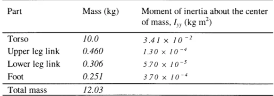
Table 1. Inertia parameters of the simulated biped

Part Mass (kg) Moment of inertia about the center

of mass, I,,. (kg m2

)

Torso 10.0 3.41 x 10 -2

Upper leg link 0.460 1.30 x 10-4

Lower leg link 0.306 5.70 x 10-5

Foot 0.251 3.70 x 10-4

Total mass 12.03

Table 2. Length parameters of the simulated biped

Description Torso

Height of center of mass referred from hip, 1c3

Upper leg link

Length of upper leg link, 12

Distance of center of mass of the upper leg from the knee joint, 1c2 Lower leg link

Length of lower leg link, 11

Distance of center of mass of the lower leg from the ankle joint, 1,1

Foot (Symmetrical)

Foot length

Distance from ankle joints to foot based

Value 0.2 m 0.42 m 0.117 m 0.42 m 0.238 m 0.15 m 0.04 m

Chapter

3 Virtual Model Control

In biped locomotion, it is generally difficult to transform from high level task specifications, such as "walk forward" to low level motion control such as the required joint torques or trajectories. Furthermore, the dynamic equations of a biped are usually of high order. Even if we can derive the dynamic equations for the biped, we still face the problem of underactuation at the ankle during single support.

In the implementation of biped walking, one common approach is to compute and command the joint space trajectories at each phase of the walking gait and this is mostly based on a desired trajectory (e.g. of the body) in the cartesian space or some pattern generators, etc.. The desired joints' trajectories can be achieved by nonlinear control techniques like computed torque control [Mitobe et al., 1995], robust

control [Tzafestas et al., 1996], adaptive control [Yang, 1994], etc.. However, this way of controlling a

biped is computationally intensive as we need to compute the inverse dynamics. To avoid such complexity, some researchers linearize the nonlinear dynamic equations of the biped and apply modern

control techniques.

The Leg Laboratory has developed a new control approach called Virtual Model Control (VMC) for the implementation of legged locomotion. The framework of this approach was well defined in [Pratt, 1995] and a comparison with other techniques like Impedance Control, Stiffness Control etc. was also included. This chapter gives a brief introduction to this approach and elaborates the details used by the biped to perform steady dynamic walking on level terrain. It will also provide a qualitative description of the control parameters. This approach will be extended to sloped terrain walking in Chapter 5.

3.1 Task characteristics and specifications for steady dynamic walking of a biped

Before we decide on the control approach to a system, it is important to first examine the desired task for the system. This thesis assumes that the task goal for the biped described in Chapter 2 is to realize a steady dynamic walking gait in the sagittal plane, while maintaining an upright posture for the torso. It also assumes that the walking gait consists of two main phases: single support and double support. Note that when the biped is in the single support phase, it is inherently unstable (just like an inverted pendulum) due to the gravity force. Thus, it is not possible to track any arbitrary trajectory as in a manipulator arm even if it is within the non-singular workspace. The stability of the biped is maintained by alternating between the left and right support phases in the right cycle.

One characteristic of natural biped walking is that the exact trajectory of the torso is not important. For example, in human walking, we usually do not specify a walking task by numbers. We simply try to maintain a generally upright position and interact with gravity and ground friction to perform stable walking. The specification for the horizontal walking velocity is always fuzzy. For example, we think in terms of "fast", "medium", "slow" motion etc.. It has been shown that a planar biped can walk passively down a gentle slope without any actuators [McGeer, 1990].

In this thesis, we specify the desired height and velocity of the torso, while keeping it in an upright position. However, the height and horizontal velocity are allowed to vary within a tolerable range. So, the next question is whether we need a very complex and precise dynamic model for the biped to achieve such specifications. The next section describes a simple method called Virtual Model Control which has been successfully implemented on a five-link planar biped permitting it to walk steadily on level ground.

3.2

Concept of Virtual Model Control

In Virtual Model Control (VMC) [Pratt, 1995], we use virtual components (e.g. springs, dampers etc.) to generate the required actuators' forces. By attaching virtual components (which usually have corresponding physical parts, for example, a spring and a damper) at some locations of the biped, the biped will behave dynamically as if the actual physical components are attached to it provided that the actuators are perfect7.

Virtual Model Control approach results in a control algorithm which examines the virtual components to obtain virtual forces from their constitutive equations. Then these forces can be transformed to the actuator space by a transformation matrix. By changing the set points of the virtual components, we create an inequilibrium to the system; it will then adjust itself so that a new equilibrium position is reached.

The main mathematical data used in this approach is the Jacobian transformation matrix which relates the force vector in one space to another space. For example, in robotics application, we usually transform a force vector F in the cartesian space to an equivalent torque vector

f

A=j T AF _(3.1)

7 Meaning the actuators have infinite bandwidth. If the actuators have finite bandwidth, then the resulting performance will still be reasonable if the desired motion stays within the bandwidth.

A

where B J is the Jacobian matrix which transforms the differential variation in the joint space into the

differential variation of B frame with respect to A frame in the cartesian space. In Virtual Model Control,

B and A frames correspond to the action frame and reaction frame, respectively [Pratt, 1995].

Equation (3.1) requires much lower computation compared to inverse kinematics and dynamics. This transformation is also well-behaved since, for a given force vector in the cartesian space, we can always obtain a corresponding torque vector in the joint space even if the robot is in a singular configuration.

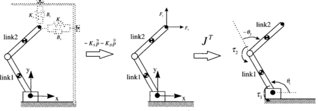
The idea of the VMC can be illustrated using a planar two-linked manipulator as shown in Figure 3. We attach two fictitious or virtual spring-dampers to the end point of the manipulator. Based on intuition,

we know that if the virtual spring-dampers have properties similar to their physical counterparts, the end position of the manipulator will settle at an equilibrium position. At the equilibrium position, the actual end-point effect of the joint torques is equal to the virtual forces of the virtual components. This is also similar to the application of the Proportional and Derivative control of the manipulator in the joint space. By shifting the set point of the virtual components, we can cause the end point of the manipulator to move to a new equilibrium position. Note that the manipulator will behave dynamically in the same way as if the manipulator had zero joints' torque and a corresponding set of real spring-dampers8 were attached at the tip. This concept is very important as it allows intuition to be applied in the VMC.

K B, F,

link2

ink2

n

linkl

-linkl link link

Figure 3. Virtual Model Control applying to two-link manipulator (Position control)

3.3 Application to steady dynamic walking of biped

In the implementation of biped walking using the VMC, the placements of virtual components require intuition; there may be more than one set of virtual components to achieve the global task defined in

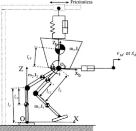
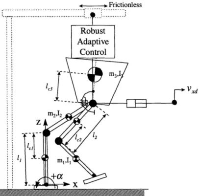
Section 3.1. Since we are interested in the motion described in cartesian space, it is natural for us to attach virtual components along each of the orthogonal coordinates in this space. One possible set of virtual components (same as those used by [Pratt, 1995]) is shown in Figure 4. A virtual spring-damper is attached to the hip along the vertical direction to generate a virtual vertical force F, at the hip. It is used to control the vertical height of the biped. A virtual damper is attached to the hip along the horizontal direction to generate a virtual horizontal force F, at the hip. This is used to control the horizontal velocity of the biped. A rotational spring-damper is attached at the hip to generate a virtual rotational force Ma about the hip. This is used to maintain the upright posture of the biped's torso. The legs of the biped are bent towards the back during walking. That is, the biped walking bears more resemblance to birds than to humans.

Though the biped has actuated ankles, we set the ankle of stance leg to be limp by commanding a zero torque. This results in a motion similar to that of the previous 5-link biped [Pratt, 1995] which had no feet. The feet of the 7-link biped simply provide better traction during the single support phase. The usage of the ankle of the stance leg to modify the walking gait is beyond the scope of the thesis, but it has been implemented in the Leg Laboratory by Jerry Pratt.

o Frictionless

z

Ic3Vxd or. d

O X

Figure 4. Virtual components used for biped walking

For our biped walking control, the inputs are the desired horizontal velocity kd (or Vxd), the desired vertical height of the hip Zd and the desired pitch angle of the body ad. All these inputs define the

desired motion of the body frame ObXbZb with respect to the inertia frame OXZ. Assuming the virtual components are linear, we can obtain the following control law in the cartesian frame:

Fx:= bx (id - X) (3.2)

F:= kz (Zd - z) + bz (Zd - i) (3.3)

Ma:= ka (ad - a) + b (ad - a) (3.4)

where bi and ki are the damping coefficient and the spring stiffness, respectively for the virtual

components in i (= x, z or a ) coordinate.

However, this set of virtual components can only be applied to the double support phase and not to the single support phase. During the single support phase, since we have set the ankle of the stance leg to be limp, the biped loses one actuated degree of freedom. Thus, one of the virtual components cannot be realised. We chose to maintain the vertical and rotational spring-dampers and let the interaction between gravity and these virtual components dictate the horizontal velocity during this phase.

The virtual forces for both the single and the double support phases are transformed into the joint space using the equations derived in [Pratt, 1995]. A list of the equations can be found in Appendix A. Realtime control of the biped locomotion can be implemented based on a state machine and the equations. In this way, the VMC enables the biped to walk without computing the inverse dynamics and kinematics and hence simplifies the computation significantly.

3.3.1 Walking control using the state machine

The pattern of events, states, and state transitions of the biped walking can be represented by a state

diagram (Figure 5). The states listed in Table 3 are used to identify distinct phases of control in a walking

cycle. A software finite state machine is used to synchronise the state transitions by monitoring for some specified conditions in the sensory data. Note that such implementation provides organised handling of the sensory data, but it does not provide a foolproof solution unless we include all the possible discrete states in the algorithm.

Table 3. Descriptions of the states used in the biped walking control

State Description

1. Double Support 1 Both feet are on the ground. Right foot is in front. 2. Right Support 3. Single-to-Double Transition 1 4. Double Support 2 5. Left Support 6. Single-to-Double Transition 2

The right foot is the stance leg and the left foot is the swing leg. Neither switch of the left foot is activated. The distance between the swing leg and the stance leg is less than the step length.

This is the intermediate phase where Right Support state transits to Double Support 2. Both feet are on the ground. Left foot is in

front.

The left foot is the stance leg and the right foot is the swing leg. Neither switch of the right foot is activated. The distance between the swing leg and the stance leg is less than the step length.

This is the intermediate phase where Left Support state transits to Double Support 1.

1. One of the limit switches of the swing foot is activated; or

2. The step length is reached

3.3.2 Swing leg strategy

In the steady walking control considered in this thesis, the objective of a swing leg strategy is to achieve approximately the desired step length. When the swing leg touches down, we also want the vertical projection of the hip to be approximately at the center between the feet. The two key variables of the swing leg task are the desired step length st and the desired lift height hI. These two variables will

be discussed in the next subsection. The detailed control strategy for the swing leg is beyond the scope of this thesis.

3.3.3 Key parameters

This section highlights the key parameters that may affect the walking pattern and performance of the planar biped. They are mainly divided into gaits' (Table 4) and virtual components' (Table 5) parameters. This subsection provides a qualitative discussion of these parameters.

Table 4. Gaits' parameters

Parameter Notation

Desired pitch angle of the torso ad

Desired hip height Zd

Desired horizontal velocity of the hip Vxd

Desired step length st

Distance from the front ankle at which double 1,

support phase transits to single support phase Swing leg :

a) Desired lift height h,

b) Swing time t1

Table 5. Parameters of virtual components

Parameter Notation

1. Spring stiffness (in z direction) kz

2. Damping coefficient (in z direction) bz 3. Damping coefficient (in x direction) bx

4. Spring stiffness (in a direction) ka

i) Desired pitch angle of the torso, ad

This variable is used directly by the torsional virtual spring-damper. The simulated biped has a torso whose center of gravity is above the hip joints. By changing the maintained pitch angle of the torso, the projection of the overall biped's center of gravity can be shifted. When ascending a slope, the natural reaction for a human is to lean forward. When descending a slope, he naturally leans back as depicted by the photographs in [Muybridge, 1989]. However, to simplify matters, the desired pitch angle of the torso is set at zero degree in this thesis regardless of the slope gradient.

ii) Desired horizontal velocity at the hip, vxd

In biped walking, several approaches can be adopted to maintain the desired horizontal velocity. For example, we can control the horizontal velocity of a biped by foot placement [Raibert, 1986] as in the case of a hopping machine. In walking, we have a period where both feet are on the ground (double support) and this also can be utilised for horizontal velocity control.

In the previous analysis, we utilised a horizontal virtual damper to correct the horizontal velocity. Since the ankle torque is zero, the biped can only have this control (without sacrificing the vertical height and body pitch control) when it is in the double support phase. To prevent the divergence of the horizontal velocity, we want the double support duty cycle to be as large as possible. However, this approach to maintain the horizontal velocity may not be effective if the walking speed is high. This is because the actual duration of double support is very short during high speed walking. Also, although the equations developed in [Pratt, 1995] assumed that full horizontal force can be achieved during double support, this is not true in real applications since the foot of the biped is not hinged to the ground. Thus, we need to set a limit to the horizontal virtual force due to the virtual damper.

We can also modulate horizontal velocity by varying the transition position from double to single support. In single support, we want to have a swing leg control strategy that minimises the disturbance to the horizontal velocity.

iii) Desired hip height, Zd

If the biped is in double support phase, the desired hip height is defined with respect to the ankle joint of the back supporting leg. Otherwise, it is defined with respect to the ankle joint of the stance leg. This variable is used by the vertical virtual spring-damper to compute the desired vertical force at the hip. At the singular configuration in which the stance leg or one of the legs during double support is fully

straightened, although the transformation equations do not "blow up", the dynamics of the system is unpredictable. Thus, it is very important to select a proper hip height so that the leg of the biped will not reach the singular configuration. The upper limit is set by the geometry of the legs and the desired step length. This variable should not be too small since it will increase the required knee torque and hence the the energy to maintain the biped's height. This is due to the increase in the moment arm of the body weight with respect to the knee joints. Thus, we would like to have this variable close to the upper limit but not reaching it.

In the algorithm, the upper limit of the hip height zli,,,it was computed as in Equation (3.5):

Zlimit = (l +12 )2 _ 12 (3.5)

where I = s, + It , sl is the desired step length and 1, is the distance from the front ankle at which the

double support phase transits to the single support phase.

We usually set the desired height at a fraction of this limit (using a factor kheight=0.8-0.9) to cater to any discrepancy in the actual hip height and the actual step length. This will also allow the biped to better accommode unknown terrain variations. Note that the foot's dimension is ignored in the computation since we compute everything with respect to the cartesian frame attached to the ankle.

11+12

Figure 6. Geometric constraint for calculating Zlimit

iv) Desired step length, st

This variable is used to plan the trajectory of the swing leg. It is coupled to the hip height as discussed before. We usually choose a desired step length depending on the lengths of the legs' links. In our present approach the double support phase is used mainly to correct the horizontal velocity. The step

length affects the relative period of the double support phase compared to the single support phase. Thus, this parameter indirectly affects the "controllability" of the horizontal speed of the locomotion.

v) Distance from the front ankle at which double support phase transits to single support phase, 1, This is the projected horizontal distance of the hip from the ankle of the front leg where the biped changes from the double support phase to the single support phase. It should be forward enough so that the biped will not lose too much energy during the single support phase, otherwise it may lose all its forward momentum. It should not be forward to the extent that the forward velocity increases excessively after a single transition. The walking cycle may become unstable if the transition position is not properly selected.

vi) Lift height, hi (For swing leg control)

This variable corresponds to the maximum lifting height of the swing leg during the swing motion and it is used in the trajectory planning of the swing leg. It may indirectly affect the degree of disturbance on the torso created by the swing leg. Its value is critical if the premature landing of the swing leg (e.g. in stair climbing) is undesirable.

vii) Swing time, ts (For swing leg control)

This variable corresponds to the time available for the biped to swing its leg during the single support phase. This is calculated approximately from the velocity at the hip before the double to single support transition. As discussed in subsection 3.3.2, we want the hip of the torso to be roughly at the center, between the front and back supporting legs at touch down of the swing leg.

viii) Parameters of the virtual components

These parameters are tuned by trial and error. Some intuition based on the linear system helps too. For example, for the vertical virtual spring-damper, we would like to have sufficiently high spring stiffness for a sufficiently quick response. The damping coefficient is then adjusted so as to achieve overdamped response. The tuning process can be iterated if required. In actual implementation, the response of the virtual component is limited by the bandwidth of the actuators. Such an approach for tuning also applies to the rotational virtual spring-damper. Note that although the virtual spring-dampers are linear components, the resulting dynamic system is nonlinear. Hence, it is not desirable to have oscillatory motion in the resulting system as nonlinear oscillatory motion can be non-intuitive.

The tuning of the horizontal virtual damper is less stringent. It can be tuned after the other virtual components are done. As mentioned before, we have to set a limit to the virtual horizontal force generated by this virtual damper because the feet are not hinged onto the ground.

Chapter

4 Robust Adaptive Control

4.1 Background

In the walking control of the planar biped, the previous chapter has demonstrated that a virtual spring-damper in the vertical direction can be used to control height. In the actual implementation, a constant offset term is added to compensate for the effective weight of the biped as perceived at the hip so that the biped can maintain close to the desired hip height without having a stiff virtual spring. However, it is not able to adapt to a varying torso mass which may occur if it carries an external load. For example, the biped will walk with a lower height if the torso's weight is increased. A possible solution would be to apply adaptive control in the joint space [Yang, 1994]. However, the inverse dynamics of a biped even in the planar case is very complex. This is complicated by the fact that in the single support phase, we lose an actuated degree of freedom at the ankle especially if the ankle is limp. Inspired by the VMC approach, this chapter will perform a feasibility study of the replacement of the existing vertical virtual component

by Robust Adaptive Controller developed by [Slotine and Coetsee, 1986]. The purpose is to enable the

biped to adapt to varying mass and walk with a height close to the desired value. The following sections will describe the theory of Robust Adaptive Control and how it can be applied to our biped to maintain its hip height.

4.2 Theory

This section includes the basic theory of Robust Adaptive Control. Since we are interested in a dynamics problem which is governed by the Newton's Second Law, let's consider the following second order nonlinear equation:

ali +a2f (-,x) +a3g(x) +d(x, i,t) = u (4.1)

where a,, a2 and a3 are unknown constants, f (, x) and g(x) are nonlinear functions, d(x,i,t) is

the disturbance of known bound D (i.e.

Idl

Definitions:

where Z~ = z - Zd ,r , = Xd - AXj and )A is a strictly positive constant.

s(t)

sa (t) = s(t)- Osat( o?) (4.3)

The goal of the control is to make SA =- 0 such that s is bounded by . It can be shown that [Slotine

and Li, 1991]

Vt _ 0,

Is(t)

Vt ;2 0,

'

(t) 5 (2); -', i=0,1.

To ensure that SA (co) -4 0, let's define

Y=[ir f(jC, x) g(x)],

=[a, a2 a3 ]

a =a-a.

where d is the estimate of d . We can choose the following Lyapunov candidate function

a, 2 1

r-V= -SA +a 2 .

2 2 (4.5)

where F is a symmetric positive definite constant matrix. The time derivative of V is then given by

V= aIsA s+ F-la

= sa (al-a1xr)+aTF-la

=s (u-a 2f -a 3g-d-alir)+ a - i

Let's define the control law as

u = Ya - ks (4.6)

where k is a strictly positive constant. Then

V = sY -sad-ksAs+'Tr-' .

By setting sY+aTF-' = 0, we obtain the adaptation law

Thus, 1 becomes

s V = -sAd - ksA (sA + sat( ))

=-sAd - ksA 2 -ks

By setting ko = D , the resulting expression of V is

V < -ks 2 (4.8)

By Barbalat's Lemma [Slotine and Li, 1991], we can show that s, - 0 as t - oo.

4.3 Application of Robust Adaptive Control to biped walking

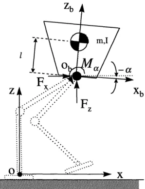
Based on the massless leg model as shown in Figure 7, we apply Robust direction dynamic equation of the biped as shown below:

m + mg+d( ,,t)= Fz

Adaptive Control to the

z-(4.9)

where m is the effective mass of the biped observed at the hip,

j

9,

is the disturbance term which includes the variation9 of the effective inertia and the effect of the swing leg dynamics. Note that the resulting system in the z-direction can be viewed to be a new "virtual component" for the VMC (Figure 8) which generates Fz, while the other two variables (vxd and ad ) are still controlled using the virtual components described in Section 3.3.

Definitions: ir = id - Az ,where Z = Z - Zd s = Z + = i - i, (4.10) (4.11) (4.12) (4.13) SA = s - sat(-) Ya = (zr + g)m where a = m and Y = (Zr + g)

The following control law (Equation (4.14)) and adaptation law (Equation (4.15)) are used:

F, = Ya - ks

a = -YTsA

(4.14) (4.15)

where y is a strictly positive scalar.

Note that, on level ground walking, zd = 0 and id = 0. The following section study the effects of each variable ( A , k, y , D, Aro10) used by this Robust Adaptive Controller.

ZA

_Xb

FZ

'''

~'''

~

Figure 7. Massless leg model for the biped

10 This variable is the initial estimate for m.

F ..

.

:::! .i-ii

..

.

'

'

..- Frictionless ... .. . ..

...

Robust

Adaptive

Control

Figure 8. Robust Adaptive Control applied to z-direction

4.4 Simulations results

In this section, the effects of the parameters ( ; , k, y, D, M^o) described in the previous section are

studied based on level ground walking simulation of the biped. In all the simulations, the desired height of the hip was fixed at zd=0.7 m, the desired horizontal velocity was fixed at vxd=0.4 m/s and desired pitch angle was fixed at ad = 0. The initial conditions of the simulation were assigned to be the same as the desired value. The desired step length of the biped was fixed at 0.28 m.

4.4.1 Effect of a.

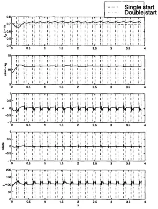
We first varied A, while setting the other parameters as follows: k=50, y =10, D-5, ri, =9. The simulation results for A =0.2, 2, 5 and 10 are shown in Figure 9, Figure 10, Figure 11 and Figure 12, respectively.

Theoretically, when s, - 0, will converge toward the bound (O/A) (Equation (4.4)). Since = D/k and both D and k were fixed in these simulations, large A would result in small j . This is

demonstrated to be true by comparing the top graph of Figure 9, Figure 10, Figure 11 and Figure 12. Note that A also behaves like the ratio of the proportional gain over the derivative gain in a PD controller. However, in a real system, A is limited by the structural resonant modes, neglected time delays and sampling rate [Slotine and Li, 1991]. Furthermore, for biped locomotion, the foot is not fixed to the ground like that of a manipulator. So, we do not want A to be too high.

From the top graph of Figure 9, we observed that when A. was too low, the bound (= /A) for

" became too big (Equation (4.4)) and the hip height fluctuated significantly. Due to the large fluctuation in the hip height, the biped's leg(s) reached singular configuration and resulted in instability.

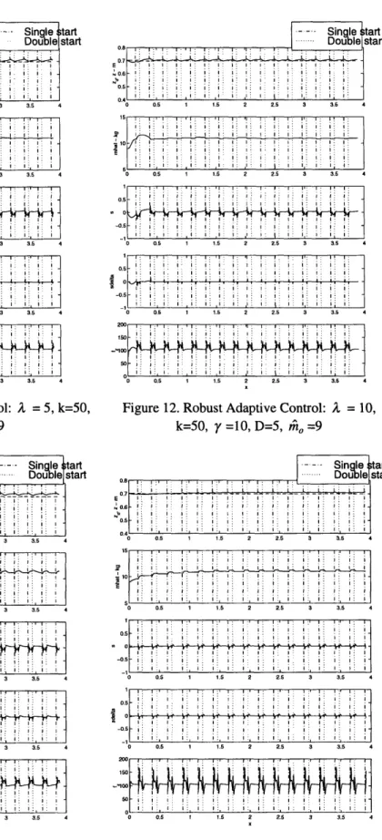
It was observed that for all A' s used here, Z did not seem to converge to within the bound (given by O/A ). This might be due to the fact that the disturbance bound D we set was too small compared to the real disturbances (e.g. due to the swing leg dynamics). That is, the results of the theoretical analysis we have done do not hold if selected D is smaller than the actual D. Interestingly, it was also observed that for A. =2, Z remained positive after the transient response had subsided.

Since we have mentioned that in our biped walking control, exact trajectory tracking is not important, the result of A, =2 is acceptable and we set A =2 for the subsequent simulations. Besides, if A is too high, it may cause the biped to be unstable if it walks on rough terrain.

4.4.2 Effect of

k

Equation (4.14) shows that the value of k influences the effect of s on F. k also directly affects

#

(=D/k), which in turn affects the bound for Z as discussed before. This subsection compares the

simulation results of Figure 10, Figure 13 and Figure 14 to study the effect of k. The top graph of these figures verifies that as value of k increases, the bound for " becomes smaller. Large k also improved the transient response of Z because it acts like a gain to the controller. However, when k was increased, the variation in the control input F, was very high and abrupt (see the graph of F, vs x in Figure 10, Figure 13 and Figure 14). Such variation in F, may not be achievable in a real system if the required bandwidth is much larger than the actuator's bandwidth. Also, high k will retard the adaptation rate for

i

4.4.3 Effect of D

The parameter D has direct influence on

4

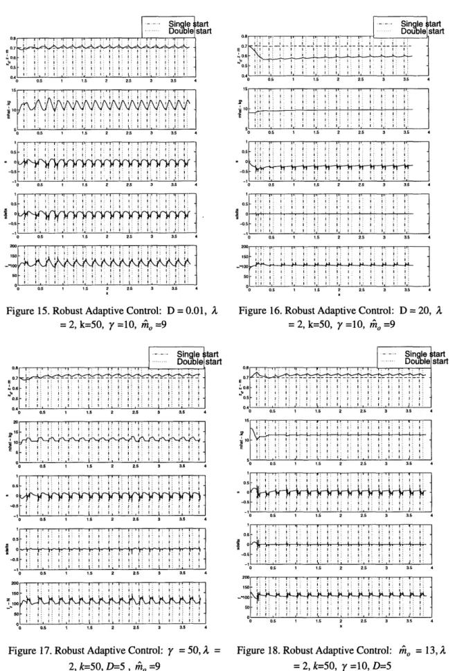
to be small. However, D is determined by the actual disturbances. To study the effect of D, this subsection looks at the simulation results shown in Figure 10, Figure 15 and Figure 16.

Comparing the top graph of Figure 10 and Figure 16, the results demonstrated that when D was large, it indeed allowed a greater variation in Z . Also, for the sA plot, we observed that the larger was D, the "quieter" was SA after the initial transient response.

For very small D as in Figure 15, we observed that

A

4.4.4 Effect of

y

y appears in Equation (4.15) and hence it is one of the parameters which affects the adaptation rate for A . It behaves like the gain of an integral controller. This subsection compares the simulation results between Figure 10 and Figure 17.

For higher y (Figure 17), it was observed that Z was smaller at the transient portion. This was because A was being updated at a faster rate. However, after the transient portion of the response was over, Z seemed to having the same behaviour and bound as shown in both figures. It was also observed that for high y , A became rather oscillatory (comparing the graph of A vs x in Figure 10 and Figure

17).

4.4.5

_{Effect of}

_r;

This subsection studies the capability of the biped to adapt to step change (for example, due to loading and unloading of carried item) in effective mass. Instead of changing the effective mass (about 11 kg) of the biped, we changed M^o (the initial value for A ) so that it differed from the actual effective mass.

When zo is smaller than actual effective mass (see Figure 10 where -o =9kg), it corresponds to the

instance when the biped just loads itself with an external load. When -o, is greater than actual effective

mass (see Figure 18 where

At

changes in effective mass for both unloading and loading of an external load which was about 18% of the effective mass.

Note that the actual effective mass deviates from body mass (=10kg) because the former includes the effective mass of the leg(s) too. In the biped walking simulation, although we know the body mass, we do not have ready information about the effective mass of the leg. We need to obtain the inertial mass matrix referred to the hip and this is cumbersome. The properties of Robust Adaptive Control allows us to absorb part of the effective mass of the legs into t and treat the rest of which as a disturbance.

--- Single _-tart Double start 0.7 -I : II 0 02 04 06 08 1 12 14 16 1 2 0 0 02 I 04 06 OB 1 1.2 1 6 1.8 2 0 0.2 0.4 0.6 0.8 1 1.2 1.4 16 1.8 2 0E

H

Figure 9. Robust Adaptive Control: A =0.2, k=50,

7 =10, D=5, i^ o=9 ... _{Single tart} Double start 0.6 0.6 I I: 0.5 I I I 0 0.5 1 1.5 2 2.5 3 3.5 4 10 0 0.5 1 1. 2 2.5 3 3.5 4 0

1

Figure 10. Robust Adaptive Control: = 2,

0 0. k=50, 1.5 2 2.5 3 3.5 4=9

Figure 10. Robust Adaptive Control: . = 2,

... Single tart Double start 07 I I II Il 05 i i 0.4 0 0 5 1 : I 0 0.5 1 1.5 2 2.5 3 3.5 4 S i i ! i I i l i i j i i i i i iI I I o : I . 10 I: I I I i : i i 0 i : i : i: : i : : I 0 0.5 1 1.5 2 2.5 3 3.5 4 S I i I: i I I: _I i: I: _I I _Ii S I i I i i I I i: I -0.5-& 1 1 . *• I I • - ,: I •I 0 0.5 1 1.5 2 2.5 3 3.5 4 1 0 i l l i i t i I: i I : i :i i i i i l i ii 0 0.5 1 1.5 2 2.5 3 3.5 4 x - . Single tart S... Do le start 0.6 0.4 0 05 1 5 2 25 3 3. 4 0 05 1 20 3 30 0.5- : I; I:I I 100 0.5 _a 1 1.5 _I 2 2.5 3 3.5 4 SI . I I I: i il: I: I:t I I I : 0 0.5 1 1.5 2 2.5 3 3.5 4 x

Figure 11. Robust Adaptive Control: A = 5, k=50, Figure 12. Robust Adaptive Control: A = 10,

y =10, D=5, i o=9 ... _{Single tart} ... Double start 0 ; i i i I I I i i i i I I: I 0 05 1 1. 2 25 3 35 4 S I I I I I I I I I I I I 0 05 l l l l4l 0 m m 0 _I 0.5 1 1.5 2 2.5 3 3.5 i: I I : I I I I I I I i I i I I I I ii i ii i I i i I: I: i i : i i i i: 0 0.5 1 1.5 2 2.5 3 3.5 4

Figure 13. Robust Adaptive Control: Ik 100,

Si i i: i i i, i i I =9 i l l I I i l l i i 0 0.5 1 1.5 2 2.5 3 3.5 4 A=2, y= 10,D=5, mo=9 k=50, y =10, D=5, -o4 =9 ---- _{Single art} ... Dou le start 0.7 0. : : i : i i S0.5 0.4 0 0.5 1 1.5 2 2.5 3 3.5 4 0 0.5 1 1.5 2 2. 3 3.5 0 0.5 1 1.5 2 2.5 3 3.5 4 S - I I I I. . I 0 .5 1 1.5 2 2.5 3 3.5 4 10 0 o 0.5 1 1.5 2 2.5 3 3.5 4 x

Figure 14. Robust Adaptive Control: k = 500,

S Single tart Double start - 1 1 1 1 1 1 1 1 1 10 4_{o i}i _{I I : : i i} 0 05 1 _{I I: :} 15 _{1 i : i i} 2 25 _{ii i ii ii iii}3 35 4 S I I I E _{0 0.5 1 1.5 2 2.5 3 3.5} 4 S0.5 1 1 5Il I I I I 0 0.5 1.5 2 _{Fi u} 2.5 _{I 5. 1: I} 3 _{I ; I I}3.5 4 - I I I I i I I: I : I I I I 0 = 2, k= 50, y =10, , = 9 S0.7 1 1 - I : I I i I: i: i i: r i i Ii IIi ii I 0 0.5 1 1.5 2 2.5 3 3. 5 4 00k=1 2 m 3549 00 _{co .7 :: i i i i i ! " I i: : i I "i ": i :} so--S I I II I I I: I 0 0.5 1.5 2 2.5 3 .5 4

Figure 17. Robust Adaptive Control: y = 50 A = 2, k=50,D 5 , ink 9 0.8 . : : : 0 0.5 1 1.5 2 2.5 3 3.5 4 0 0.5 1 1.6 2 2.5 3 3.5 4 -1 I 1 I1 I[ I I: I m I 1 I : I [ 1 : I I 0-01 . .5 . 1 .. 2 2. 3. 3. 4 2, k=50, D=5 , ,'ro =9 .. Single tart Double start 0.8 0. I I I 0.0-I I II 0.4 10 S I liI I I I I I i I 0 . 0.5 II: I I . I: -03 0.50 I: I : I I : -0. i- I .I I 0 0.5 1 I -I : i : i i 1.5 i ,: ' i,: i' : ',: I: I I I: i i I. I I I . I .' I. I. I ii 2 i: ii i ii 2.5 3 3.5 1:50 I I I II I I I I I I - -- Single start ... Double start 0.8 0.7 ---15 0 05 1 1.5 2.5 3 3. 4 -0. ii i i i ii i i i 0 0.5 1 1.5 2 2.5 3 3.5 4 . 10

~

Figure 18. Robust Adaptive Control: ho = 13, A

= 2, k=50, y =10, D=5

4.5

Discussion

One may ask whether we can simply use PID controller instead of the more complex Robust Adaptive Controller. We would say that a PID controller will probably work fine too. Nonetheless, we think that Robust Adaptive Controller is better because it provides the information of the effective mass. Furthermore, the computation of Robust Adaptive Controller is not very intensive and hence it is worthwhile to implement Robust Adaptive Controller for our purpose. In fact, when the estimation of m has stopped and all other transient behaviors have settled down, Robust Adaptive Controller behaves like a virtual spring-damper with a constant offset term (Equation (4.14)).

If the legs are heavy, we may split the adaptation parameters into two parts, one for the single support phase and the other for the double support phase because the effective mass for the two phases may deviate substantially from one another.

4.6 Conclusion

This chapter has demonstrated successful application of Robust Adaptive Control to biped walking on level ground in the simulation. The effects of the parameters were also studied. It is concluded that Robust Adaptive Controller is applicable for steady biped walking and it enables the biped to adapt to about 18% step change in body mass. The computation requirements for such a controller are very low and do not defeat the original purpose of using the VMC. Thus, Robust Adaptive Controller can be a virtual component candidate for the VMC. Chapter 6 will demonstrate the robustness of this approach by simulating the biped walking over a series of unknown slopes.