Publisher’s version / Version de l'éditeur:
Vous avez des questions? Nous pouvons vous aider. Pour communiquer directement avec un auteur, consultez la première page de la revue dans laquelle son article a été publié afin de trouver ses coordonnées. Si vous n’arrivez pas à les repérer, communiquez avec nous à [email protected].
Questions? Contact the NRC Publications Archive team at
[email protected]. If you wish to email the authors directly, please see the first page of the publication for their contact information.
https://publications-cnrc.canada.ca/fra/droits
L’accès à ce site Web et l’utilisation de son contenu sont assujettis aux conditions présentées dans le site LISEZ CES CONDITIONS ATTENTIVEMENT AVANT D’UTILISER CE SITE WEB.
CCWI2007 SUWM2007 Conference [Proceedings], pp. 1-8, 2007-09-03
READ THESE TERMS AND CONDITIONS CAREFULLY BEFORE USING THIS WEBSITE. https://nrc-publications.canada.ca/eng/copyright
NRC Publications Archive Record / Notice des Archives des publications du CNRC :
https://nrc-publications.canada.ca/eng/view/object/?id=5bec181f-a7d6-45fd-8dbd-96ca0e2f7f91 https://publications-cnrc.canada.ca/fra/voir/objet/?id=5bec181f-a7d6-45fd-8dbd-96ca0e2f7f91
NRC Publications Archive
Archives des publications du CNRC
This publication could be one of several versions: author’s original, accepted manuscript or the publisher’s version. / La version de cette publication peut être l’une des suivantes : la version prépublication de l’auteur, la version acceptée du manuscrit ou la version de l’éditeur.
Access and use of this website and the material on it are subject to the Terms and Conditions set forth at
Static and dynamic effects in prioritizing individual water mains for renewal
http://irc.nrc-cnrc.gc.ca
S t a t i c a n d d y n a m i c e f f e c t s i n p r i o r i t i z i n g
i n d i v i d u a l w a t e r m a i n s f o r r e n e w a l
N R C C - 4 9 6 7 2
K l e i n e r , Y . ; R a j a n i , B .
A version of this document is published in / Une version de ce document se trouve dans: CCWI2007 SUWM2007 Conference, Leicester, UK., Sept. 3-5, 2007, pp. 1-8
The material in this document is covered by the provisions of the Copyright Act, by Canadian laws, policies, regulations and international agreements. Such provisions serve to identify the information source and, in specific instances, to prohibit reproduction of materials without written permission. For more information visit http://laws.justice.gc.ca/en/showtdm/cs/C-42
Les renseignements dans ce document sont protégés par la Loi sur le droit d'auteur, par les lois, les politiques et les règlements du Canada et des accords internationaux. Ces dispositions permettent d'identifier la source de l'information et, dans certains cas, d'interdire la copie de documents sans permission écrite. Pour obtenir de plus amples renseignements : http://lois.justice.gc.ca/fr/showtdm/cs/C-42
Static and dynamic effects in prioritizing individual
water mains for renewal
Yehuda Kleiner and Balvant Rajani
Institute for Research in Construction, National Research Council, Ottawa, Ontario, K1A 0R6, Canada
ABSTRACT: The physical mechanisms that lead to pipe breakage are often very complex and not well un-derstood, and data on the physical condition of pipes is scarce. Conversely, many water utilities do maintain records of pipe failure (or repair) events, which can be used for the statistical analysis of breakage patterns to discern the deterioration of water mains.
The structural deterioration of water mains and their subsequent failure are complex processes, which are af-fected by many factors, both static (e.g., pipe material, size, age, soil type) and dynamic (e.g., climate, ca-thodic protection, pressure zone changes). Several models exist in the literature, which use various statistical methods to analyze breakage patterns of pipe breakage histories. Some of these models were designed to ad-dress individual water mains, while others can handle only relatively large groups of pipes, which are pre-sumed to be homogeneous with respect to their deterioration patterns. Dynamic factors can currently be con-sidered only in one a model that was designed to deal with pipe groups. While group deterioration analysis is important for high-level renewal planning, operational considerations require the prioritization of individual pipe for renewal within such groups.
The National Research Council of Canada (NRC), with support from the American Water Works Association Research Foundation (AwwaRF) is undertaking research to develop an approach that will allow the consid-eration of dynamic factors that influence the breakage patterns of individual water mains. This research is en-tering its third year and in this paper we provide some interesting interim insights and results.
1 INTRODUCTION
The structural deterioration of water mains and their subsequent failures are complex processes, which are affected by many factors, both static (e.g., pipe material, size, age, soil type) and dynamic (e.g., cli-mate, cathodic protection, pressure zone changes). Limited knowledge and scarcity of data render the physical modeling of all distribution water mains impractical. In contrast, statistically derived empiri-cal models can be useful for small-diameter water mains for which low cost of failure does not justify expensive data acquisition campaigns.
Statistical methods to predict water main breaks use available historical data on past failures to iden-tify pipe breakage patterns. These patterns are then assumed to continue into the future in order to pre-dict the future breakage rate of a water main or its probability of breakage. Statistical methods can be classified broadly into deterministic, probabilistic multi-covariate and probabilistic single-covariate (namely time) models. These models are typically
applied to grouped data (Kleiner and Rajani, 2001). Deterministic models predict breakage rates using two or more parameters, based on pipe age and breakage history, e.g., Shamir and Howard (1979), Walski and Pellicia (1982) and Clark et al. (1982). Many factors, operational, environmental and fac-tors dependent on pipe material, jointly affect the breakage rate of a water main. The population of water mains has to be partitioned into groups that are appreciably uniform and homogeneous with re-spect to these factors, in order for two or three pa-rameters to capture a true breakage pattern. The par-titioning of data into groups, however, warrants careful attention because two conflicting objectives are involved. On one hand the groups have to be small enough to be uniform but, at the same time, the groups have to be large enough to provide results that are statistically significant. Probabilistic multi-covariate models, such as those based on the propor-tional hazards statistical model (e.g., Andreou et al., 1987; Eisenbeis, 1994) or on non-homogeneous Poisson process (e.g., Constantine and Darroch, 1993; Røstum, 2000), can explicitly and
quantita-tively consider most of the covariates in the analysis. This ability makes them potentially powerful to pdict future breakage rates of water mains. It also re-duces the need to pre-partition the data into groups, although often some level of partitioning may still be required. Other types of approaches include ac-celerated failure time (Røstum, 2000) and models that attempt to fit probability distributions to inter-break time durations in pipes, e.g., Gustafson and Clancy (1999), Mailhot et al. (2003) and Dridi et al. (2005).
All the models described above can only deal with static covariates. Water utilities have observed that operations such as pressure control, cathodic protection (both systematic (retrofit) and opportunis-tic (hot spot)) and external environment (water tem-perature and soil moisture deficit) can have a sub-stantial impact on water main failure patterns. Neglecting to account for these effects can lead to inaccurate conclusions, which result in sub-optimal renewal strategies. Kleiner and Rajani (2000, 2004) proposed a model that considers both static and dy-namic influences on the breakage pattern of water mains. It is a deterministic model, which works only with groups of pipes. In this paper we report on in-terim results of research intended to extend this model to consider individual (rather than groups of) water mains to enable effective prioritization of the renewal of these individual water mains.
The rest of this paper is organised as follows: Section 2 provides an introduction to the analysis of historical breakage patterns of groups of water mains, with the consideration of time-dependant (dynamic) effects. Section 3 describes on-going re-search on ways to “explain” variations in breakage patterns of individual mains, and Section 4 provides a summary and direction of further research.
2 MODELLING DYNAMIC EFFECTS ON BREAKAGE PATTERNS OF GROUPS OF PIPES
The model proposed by Kleiner and Rajani (2000, 2004), named D-WARP (Distribution Water mAins Renewal Planner), addresses the deterioration rates of a homogeneous group of distribution water mains. It considers time-dependent (dynamic) factors such as temperature (in the form of freezing index), soil moisture (in the form of rainfall deficit), and ca-thodic protection (CP) strategies, including hot spot CP as well as systematic retrofit CP. Non-time-dependent (or static) factors such as pipe character-istics and soil type are implicitly considered through the formation of homogeneous water main groups. The underlying premise is that a homogeneous group of pipes experiences a steady increase in breakage rate (hereafter referred to as “background ageing rate” or simply “ageing rate”), upon which
year-to-year variations occur. Some of these varia-tions can be attributed to time-dependent factors. Once background ageing rates is discerned, it can be used to project future breakage rates. In addition, the impact of operational strategies such as schedules of cathodic protection (both hot spot and retrofit) can be superimposed on this background ageing. Subse-quently, the life cycle costs of various scenarios op-erational strategies can be evaluated and fine-tuned to achieve maximum efficiency in resource alloca-tion.
D-WARP uses a general, multi-covariate expo-nential model to discern breakage patterns while considering time-dependent factors:
T t x a t
N
x
e
x
N
(
)
=
(
)
⋅ 0 t (1)where xt = vector of time-dependent covariates
pre-vailing at time t, N(xt) = number of breaks resulting
from xt, a = vector of parameters corresponding to
the covariates x; xto= vector of baseline x values at year of reference to. Time-dependent covariates (or “explanatory variables”) can be pipe age, tempera-ture, soil moistempera-ture, number of effective CP anodes, etc. Parameters
( )
0
t
x
N and a can be found by least square regression or by using the maximum likeli-hood (ML) method.
The multi-covariate model is applied to groups of water mains that are assumed homogeneous with re-spect to their deterioration rates. Grouping of water mains is typically based on some or all of the static factors (e.g., by material type, diameter, vintage, geographical location, etc.) for which data are avail-able. Although the mathematical model is not re-stricted in the number of covariates it can consider, data availability (or rather unavailability) is usually the limiting factor. Currently the only time-dependent covariates that are considered are age, temperature, winter soil moisture, annual soil mois-ture, hotspot cathodic protection and retrofit ca-thodic protection. Freezing index is used as a surro-gate measure for annual temperature. Two schemes of rain deficit are used as surrogate measures for winter soil moisture and annual soil moisture. De-tails on these surrogate measures are provided in Kleiner and Rajani (2002).
Hot spot cathodic protection is the practice of op-portunistically installing a protective (sacrificial) anode at the location of a pipe repair. These anodes are typically installed without any monitoring and stay in the ground until total depletion, usually with-out replacement.
Retrofit cathodic protection refers to the practice of systematically protecting existing pipes with gal-vanic cathodic protection, whereby an anode is at-tached to each pipe segment (typically 6 m or 20’ length), or if the water main is electrically
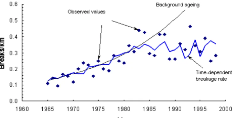
continu-ous a bank of anodes in a single anode bed is suffi-cient. Kleiner and Rajani (2004) described in detail how cathodic protection is considered in the multi-covariate model (Equation 1). Figure 1 provides an illustration of an example group of pipes for which a HS CP program was started in 1984.
The break history analysis in D-WARP provides the coefficients a for background ageing, climatic covariates and cathodic protection effects. Once background ageing has been discerned, it is assumed that the group of pipes will continue to age at the same rate. It is also assumed that the cathodic pro-tection effects observed in the past will continue to prevail if CP is continued. Based on these assump-tions a forecast of future breakage rates can be made. Note that climate effects are usually not con-sidered in this forecast because they require a credi-ble climate forecast, including temperatures and pre-cipitation
Figure 1. Breakage pattern of cathodically protected pipes (HS CP started 1984)
3 INVESTIGATING VARIABILITIES IN
BREAKAGE COUNT OF INDIVIDUAL PIPES WITHIN A HOMOGENEOUS GROUP
The ultimate goal of the research on which this paper reports is to develop an operational tool for network owners and planners to be able to prioritise individual water mains for renewal, while consider-ing both static and dynamic effects that influence pipe deterioration rates. The underlying assumption of our approach is that within a homogeneous group of pipes, some of the variations in breakage rates among individual water mains are a result of irre-ducible random natural variation (aleatory uncer-tainty), while some of the variation (epistemic un-certainty) can be explained by the existence of some factors. These factors need to be identified and sub-sequently expressed as covariates (or “explanatory variables”) in a mathematical model.
3.1 Candidate covariate: pipe length
In practically all reported analyses of breakage frequency in pipe groups (including those cited in
Section 1, as well as others), the aggregate length of the pipes in a group has been used as a normalizing factor. This has the implication that breaks are dis-tributed uniformly along the pipes, which carries the expectation that the number of breaks be directly proportional to the length of pipes. The literature also reflects that pipe length has frequently been used as a covariate capable of “explaining” at least some of the variability observed in individual water mains. Researchers (e.g., Andreou et al, 1987; Ei-senbeis, 1994; Røstum, 2000, and others) used the log transform or n-th root of pipe length as a covari-ate in their proportional hazards models. These re-searchers reported various results with respect to the “quality” of pipe length as a covariate. In some wa-ter distribution networks, length was found to be sta-tistically significant, while in others it was not. Ad-ditionally, pipe length was found to be significant for some pipe materials (CI, PVC) when the number of previous breaks was between 1 and 3, while in-significant when the number of previous breaks was 0 or equal or greater than 4. In other materials (AC) it was found to be not significant at any level of previous breaks. In some cases, when the length was found to be significant, the coefficient (in the expo-nent) was obtained with values around 0.5. This im-plied that the hazard was proportional to the square root of the pipe length. Giustolisi et al. (2005) used Evolutionary Polynomial Regression (EPR) to find polynomial expressions that predict the breakage rate of pipes. In several data sets length was found to be a good predictor.
These inconclusive results on using length as co-variate, motivated us to re-examine pipe length as a candidate covariate for explaining differences in breakage intensity of individual pipes in a homoge-neous group. The length of individual water mains is typically in the order of magnitude of no more than several hundreds of meters. A protocol was therefore developed to artificially generate pipes with a wider range of lengths:
a) Extract a homogeneous group of pipes (same di-ameter, material, vintage, cathodic protection). Total number of individual pipes in the group is
N. For each pipe i (i = 1, 2, ..., N), record its
length, li, and the number of breaks, bi, observed
during the analysis period.
b) Compute the correlation (Pearson) coefficient between li. and bi (individual pipes).
c) Set a constant, say, MaxPipes = 2.
d) Generate a positive random integer NoPipe where NoPipe ≤ MaxPipes
e) Generate NoPipe positive unique random num-bers, say k1, k2, …, kNoPipe. each of which ≤ N.
f) Record the sum of lengths Lj = Σ(lk1, lk2 …) and
g) Repeat steps (d) to (f) thousand (1000) times. We now have 1000 pairs Lj and Bj (j = 1, 2, …,
1000).
h) Compute the (Pearson) correlation coefficient between Lj and BBj.
i) Repeat steps (d) to (h) for MaxPipes = 2, 5, 10, 20, 30, 50, 100, 500 and 1000.
The protocol was applied, with similar results, to three different data sets from three major Canadian
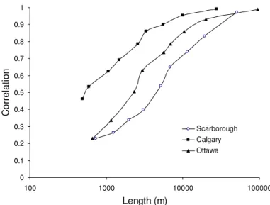
cities. Figure 2 illustrates detailed results for one of them, while Figure 3 compares the overall correla-tions for all three data sets.
Figure 2 demonstrates that while in the macro level (long pipe lengths) there is clear linear correla-tion between pipe length and number of breaks, in the micro level (shorter pipe lengths) this correlation is completely overtaken by “noise”, which is the natural variation between pipes. In fact, viewing
0 2 4 6 8 10 12 14 16 0 200 400 600 800 1000 Length (m) B reak s 0 2 4 6 8 10 12 14 0 200 400 600 800 1000 Length (m) B reak s MaxPipes = 2 Correlation coefficient ρLB = 0.354 Individual pipes Correlation coefficient ρLB = 0.302 0 5 10 15 20 25 0 500 1000 1500 2000 Length (m) B reak s MaxPipes = 5 Correlation coefficient ρLB = 0.46 0 5 10 15 20 25 30 0 500 1000 1500 2000 2500 3000 3500 Length (m) B reak s MaxPipes = 10 Correlation coefficient ρLB = 0.63 0 10 20 30 40 50 60 0 1000 2000 3000 4000 5000 6000 Length (m) Br e a ks MaxPipes = 20 Correlation coefficient ρLB = 0.73 0 10 20 30 40 50 60 70 0 2000 4000 6000 8000 Length (m) B reak s MaxPipes = 30 Correlation coefficient ρLB = 0.80 0 10 20 30 40 50 60 70 80 90 100 0 2000 4000 6000 8000 10000 12000 Length (m) B reak s MaxPipes = 50 Correlation coefficient ρLB = 0.87 0 100 200 300 400 500 600 0 20000 40000 60000 80000 100000 120000 Length (m) Br e a ks MaxPipes = 500 Correlation coefficient ρLB = 0.99 a b c d e f g h
graph a to graph h (top right to bottom left in Figure 2) is akin to zooming in on the bottom left corner of the graph a.
Figure 3. Variation of linear correlation coefficients with pipe lengths in 3 cities
It appears that the intuitive understanding that higher exposure leads to more observed breaks must be true since pipe length is a surrogate for exposure. How-ever, the natural randomness inherent in the rela-tionship between length and breaks is relatively high. Further, while pipe length is a continuous physical property, pipe break is a discrete entity. In-dividual pipes, whose length might typically vary between a few tens and a few hundreds of meters, typically do not experience too many breaks before they are replaced. This discrete nature of breakage data amplifies the natural randomness in relatively short pipes. Consequently, the randomness or the “noise” in the data all but completely overwhelms any mathematical relationship when comparing
in-dividual mains. However, when the variability in pipe lengths is big, the aggregate number of breaks becomes continuous-like in its behaviour and the natural randomness produces “noise” that is much smaller relative to the mathematical relationship and therefore no longer overwhelms this relationship. It should be noted that repeating the same exercise with powers (between zero and unity) and log of lengths yielded similar results.
While Pearson’s linear correlation was rather low between length and breaks of individual mains, Spearman’s rank correlation proved significantly higher. Spearman’s rank correlation values for the individual water mains in Ottawa, Scarborough and Calgary were 0.38, 0.40 and 0.56 compared to Pear-son’s linear correlation values of 0.23, 0.23 and 0.46, respectively. 0 0.1 0.2 0.3 0.4 0.5 0.6 0.7 0.8 0.9 1 100 1000 10000 100000 Length (m) C or re lat ion Scarborough Calgary Ottawa
3.2 Candidate covariate: pipe failure history Pipe failure history can be characterised by the num-ber of previous failures (NOPF), as well as the tem-poral pattern of these failures, i.e., recency of these failures. Models reported in the literature (e.g., An-dreou et al, 1987; Eisenbeis, 1994; Røstum, 2000) only considered NOPF as a covariate pertaining to pipe failure history. .
To investigate how NOPF can be a predictor for future breaks,, we established a reference year and defined time windows for past and future pipe breaks, WinPast and WinFuture, respectively as as illustrated in Figure 4. The number of recorded breaks in WinPast was correlated to the number of recorded breaks in WinFuture. This was done for different reference years as well as for variouse t, values of WinPast and WinFuture. Observed trends (some intuitively expected, others not as much) were:
• Correlations between total number of past breaks and total number of future breaks increases as the length of the WinPast increased.
• Correlations between total number of past breaks and total number of future break increases as the length of WinFuture increased.
• Correlations between total number of past breaks and total number of future break generally vary for different RefYears. However, these variations
depend on the lengths of WinPast and WinFuture. As WinPast and WinFuture increase, these varia-tions decrease and these variavaria-tions all but disap-pear for WinPast ≥ 10 years and WinFuture ≥ 10.
E a rlie s t d a ta
L a te s t d a ta R e fe re n c e ye a r (R e fY e a r)
R e c o rd e d b re a k
P a s t w in d o w (W in P a s t) F u tu re w in d o w (W in F u tu re )
Figure 4. Timeline to explore pipe failure history
• The correlation between total number of past breaks and total number of future when
WinFu-ture = 1 year is very small (approximately
be-tween 0 and 0.2) and varies highly with RefYear, regardless of length of WinPast. This suggests
that the possibility of predicting next year’s breakage in individual water mains, using their past number of breaks is doubtful.
• Correlations between total number of past breaks and total number of future break when WinFuture ≥ 5 years and WinPast ≥ 15 years have values approaching 0.4.
3.3 Candidate covariate: geographical clustering Water utilities often lack data that are (directly or indirectly) geographically related, such as soil data, overburden characteristics (land development, traffic loading), historical installation practices, groundwa-ter fluctuations, transient pressures, poor bedding, etc. These data, if available, may sometimes help to “explain” variations in breakage rates. Under the hypothesis that geographical clustering of historical breaks could be a surrogate for these often missing data, we examined the viability of using geographi-cal clustering of historigeographi-cal breaks as a possible pre-dictor to explain variability of breakage rates among individual water mains in a homogeneous group of pipes. The examination comprised the following steps:
a) Extract a homogeneous group of N pipes (same diameter, material, vintage, cathodic protection). For each pipe i (i = 1, 2, ..., N) record the number of breaks bti, observed at each year t in the
analy-sis period T (t = 1, 2, …T).
b) For a reference year RefYear (⊆ T), select a win-dow of historical years WinPast and a winwin-dow of future years WinFuture. WinPast comprises Tp
years, where the first year is equal to (RefYear -
Tp + 1) and the last year equals RefYear.
WinFu-ture comprises Tf years, where the first year is
equal to (RefYear + 1) and the last year equals (RefYear + Tf).
c) Based on WinPast breakage data create C geo-graphical clusters. A break belongs to cluster cj
(j = 1, 2, …, C) if its Euclidean distance from the centroid of cj is smaller than its distance from the
centroid of every other cluster cj (i ≠ j). The
clus-tering algorithm K-Means as described by Mac-Queen (1967) was used.
d) Partition all pipes into the C clusters, based on their distances from the centroids of the clusters. e) Create C clustering covariates for each pipe,
based on the pipe distance from the centroids of the respective clusters. These covariates are sup-posed to predict the number of breaks observed during WinPast.
f) Train the model on the WinPast data by finding C coefficients that minimise the sum of square
dif-ferences between observed and predicted number of breaks in WinPast.
Use the C coefficients to predict breaks for
Win-Future.
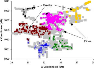
Figure 5 illustrates an example of break cluster-ing (6 clusters) in a group of cast iron 150 and 200 mm water mains, installed in Edmonton, Canada between 1902 and 1945. 5929 5931 5933 5935 5937 5939 5941 29 31 33 35 37 39 X Coordinates (kM) Y C o or di na te s ( k M ) Breaks Pipes
Figure 5. Example of historical breaks partitioned into six clus-ters
4 COMBINING EXPLANATORY VARIABLE INTO A PREDICTIVE MODEL
Based on the observations reported in the previous section, we concluded that with the given type of data it was more tenable to forecast the relative ex-pected breakage frequency of individual pipes within a homogeneous group of pipes. We therefore set out to address the following challenge: “In a ho-mogeneous group comprising N individual pipes, with available breakage history of T years, find which n pipes are expected to have the highest num-ber of breaks in the next y years”. The following procedure is proposed:
a) Select RefYear and partition the observation pe-riod T into WinPast and WinFuture. Identify n pipes with the highest number of breaks in period
WinFuture. Record these pipes in a list named Lf.
b) Similar to step (a) above, identify n pipes with the highest number of break in period WinPast and record them in a list named L1.
c) Identify n pipes with the highest length and re-cord them in a list named L2.
d) Identify n pipes that the cluster analysis predicted to have the highest number of breaks and record them in a list named L3.
e) Assign weights W1, W2, W3 to lists named L1, L2,
L3, respectively. These weights will serve as
ini-tial values to be optimized later.
f) Identify pipes that appear in lists L1, and L2 and
L3 and record these pipes in a list named L1,2,3.
Similarly, identify pipes that appear in lists L1,
and L2 and record these pipes in a list named L1,2.
List named L1,3 will comprise pipes that appear in
lists L1 and L3., and list named L2,3 will comprise
pipes that appear in lists L2 and L3.
g) If a pipe appears in a higher order list, remove it from all the corresponding lower order lists. For example, if a pipe appears in list L1,2,3 it should be
removed from lists L1,2, L1,3, L2,3 , L1, L2, and L3. In
this way every pipe will appear only once in the 7 lists.
h) Pipes in list L1,2,3 are assigned weight W1,2,3 = W1
+ W2 + W3. Pipes in list L1,2 are assigned weight
W1,2 = W1 +W2, and so on.
i) Rank all pipes (from the 7 lists) by their assigned weight in descending order. The n pipes with the highest weights are those predicted by the model to have the highest number of breaks in the future window. Record these pipes in a list LW .
j) Denote by H the number of pipes (“hits”) that ap-pear in both lists Lw and Lf.
k) Find a set of weights (Wi ; i = 1, 2, 3) that
maxi-mizes H.
This procedure was applied to several datasets and demonstrated relatively good results. For exam-ple, on a set of 1349 150 mm CI pipes (Scarbor-ough), installed between 1945 and 1960, the number of “hits” was H = 21 pipes on attempting to predict
n = 75 pipes with the highest number of breaks.
4.1 Evaluation of prediction quality
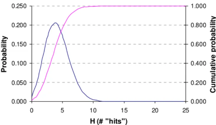
To evaluate the quality of prediction it is proposed to compare it to the probability of obtaining the same results with a random draw, i.e., what is the probability of randomly selecting n out of N pipes, so that H of the selected pipes (H ≤ n) truly belong
to the n pipes with the highest number of breaks. In our example, N = 1349, n = 75, H = 21, Figure 6 il-lustrates that obtaining more than 21 “hits” at ran-dom has virtually zero probability (1 – cumulative probability).
5 SUMMARY AND CONCLUSIONS
The analysis of historical breakage patterns in a rela-tively homogeneous group of pipes can provide in-sight into the expected future trends of the group. However, it is rarely feasible to replace an entire group of pipes due to budgetary constraints, there-fore there is a need to prioritise the replacement of
individual pipes within such a group. The first step towards prioritisation is to discern differences be-tween the individual pipes, specifically, how to pre-dict that one pipe will fail more frequently than an-other in the same group?
0.000 0.050 0.100 0.150 0.200 0.250 0 5 10 15 20 25 H (# "hits") Pr obabi li ty 0.000 0.200 0.400 0.600 0.800 1.000 C u m u la ti v e pr obabi li ty
Figure 6. Probability of obtaining results by random selection
In this paper we have reported on the examina-tion of three candidate indicators (covariates), pipe length, number of previous observed failures and pipe and break clustering. A weighted ranking – based procedure was presented, whereby these indi-cators are used to forecast the pipes with the highest number of breaks in a homogeneous group of pipes. The quality of the prediction was ascertained by comparing the prediction to random selection. More research is planned to test the procedure for consis-tency across varying time windows and reference years as well as across different data sets.
6 ACKNOWLEDGMENTS
This paper presents interim results of a research pro-ject, which is co-sponsored by the AwwaRF, the NRC and water utilities from the United States and Canada. The authors wish to acknowledge the com-petent programming help of Mr. Jeff Lalonde and the good ideas of Dr. Rehan Sadiq, both at the NRC who work in our group.
REFERENCES
Andreou, S. A., Marks, D. H., and Clark, R. M. (1987). “A new methodology for modeling break failure patterns in de-teriorating water distribution systems: Theory.” Advance in
Water Resources, 10, 2-10.
Clark, R. M., Stafford, C. L., and Goodrich, J. A. (1982). “Wa-ter distribution systems: A spatial and cost evaluation”,
Journal of Water Resources Planning and Management Division, ASCE, 108, (3), 243-256.
Constantine, A. G., and Darroch, J. N. (1993). “Pipeline reli-ability: stochastic models in engineering technology and management.” S. Osaki, D.N.P. Murthy, eds., World
Scien-tific Publishing Co.
Dridi, L,. Mailhot, A., Parizeau, M., and Villeneuve J.P. (2005) “A strategy for optimal replacement of water pipes integrat-ing structural and hydraulic indicators based on a statistical
water pipe break model”. Proceedings of the 8th
Interna-tional Conference on Computing and Control for the Water Industry, U. of Exeter, UK, September, 65-70.
Eisenbeis, P. (1994). “Modélisation statistique de la prévision des défaillances sur les conduites d’eau potable, PhD the-sis, University Louis Pasteur of Strasbourg, collection Etu-des Cemagref no 17, 1994.
Giustolisi, O., Laucelli, D, and Savic D. A., (2005). “A deci-sion support framework fro short time planning of rehabili-tation”, Proceedings of Computer and Control in Water In-dustry (CCWI), (1), 39-44.
Gustafson, J-M., and Clancy, D. V. (1999). “Modeling the oc-currence of breaks in cast iron water mains using methods of survival analysis” Proc. AWWA ACE, Chicago.
Kleiner, Y. and Rajani, B. (2000). “Considering time-dependent factors in the statistical prediction of water main breaks”. AWWA Infrastructure Conference Proceedings, March 12-15, 2000, Baltimore, Maryland.
Kleiner, Y. and Rajani, B. (2002). “Forecasting Variations and Trends in Water Main Breaks”, Journal of Infrastructure
Systems, ASCE, 8, (4), 122-131.
Kleiner, Y. and Rajani, B. (2001). “Comprehensive review of structural deterioration of water mains: statistical models”.
Urban Water, (3), 131-150.
Kleiner, Y. and Rajani, B. (2004). "Quantifying effectiveness of cathodic protection in water mains: theory," Journal of
Infrastructure Systems, ASCE, 10,(2), 43-51.
MacQueen, J. B. (1967). “Some methods for classification and analysis of multivariate observations”, Proceedings of the
fifth Berkeley Symposium on Mathematical Statistics and Probability, Berkeley, University of California Press,
1:281-297.
Mailhot, A., A. Paulin, and Villeneuve J-P, (2003). “Optimal replacement of water pipes”, Water Resources Research, 39, (5), 1136.
Røstum, J. (2000). “Statistical modelling of pipe failures in water networks”. PhD thesis, Norwegian University of Sci-ence and Technology, Trondheim, Norway.
Shamir, U. and Howard, C.D.D. (1979). “An analytic approach to scheduling pipe replacement.” J. AWWA, 71, (5), 248-258.
Walski, T. M., and Pelliccia, A. (1982). “Economic analysis of water main breaks.” J. AWWA, 74, (3), 140-147.